
The Uniform Poisson–Ailamujia Distribution: Actuarial Measures and Applications in Biological Science


Abstract
:1. Introduction
2. The Discrete UPA Distribution
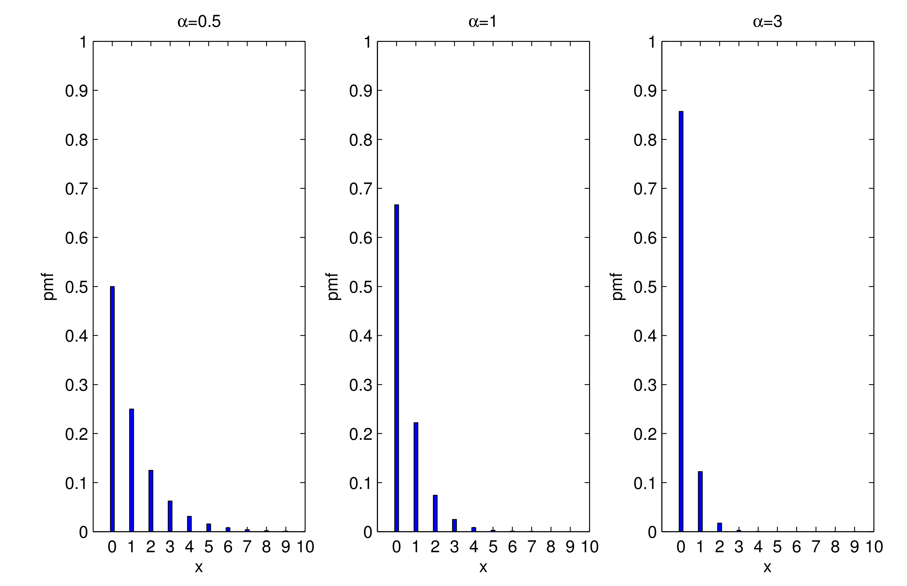
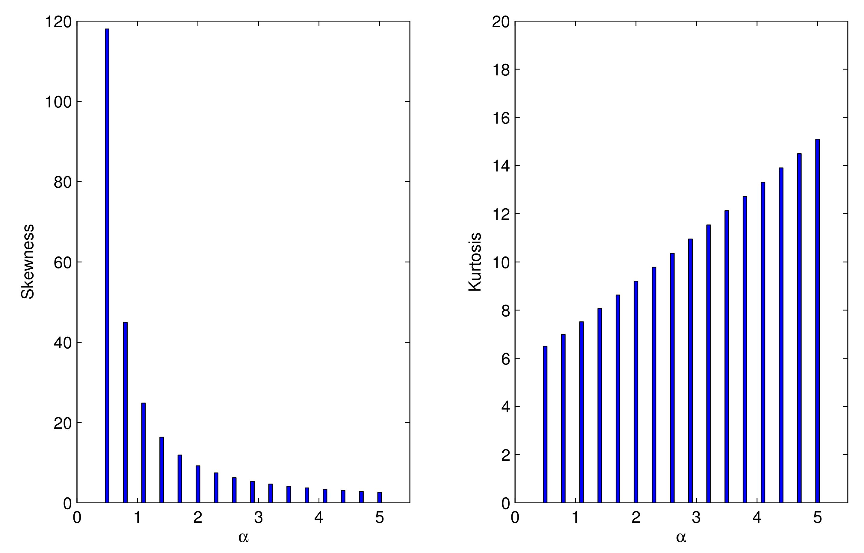
2.1. Properties
2.2. Stochastic Orders of the Parameter
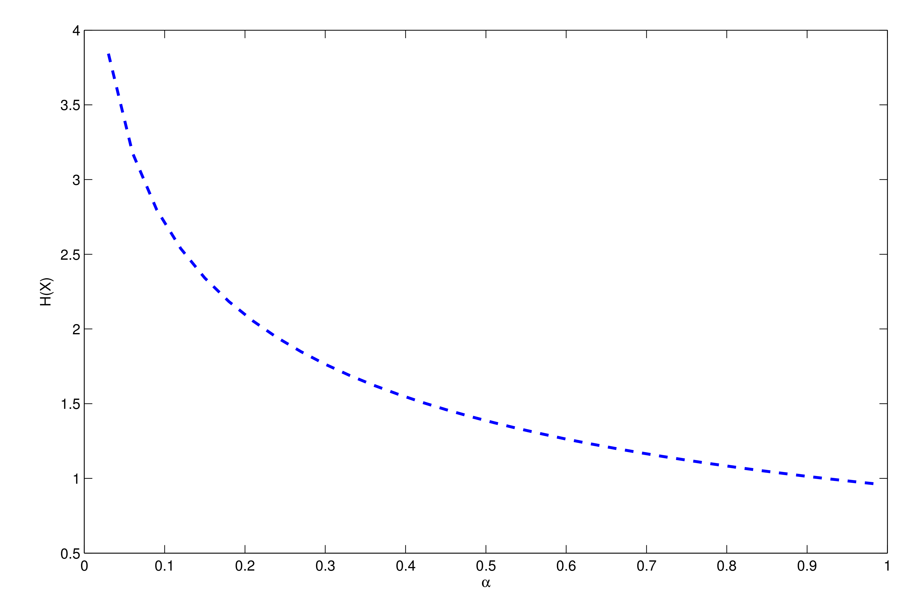
2.3. Entropy
2.4. Quantile Function
3. Actuarial Measures
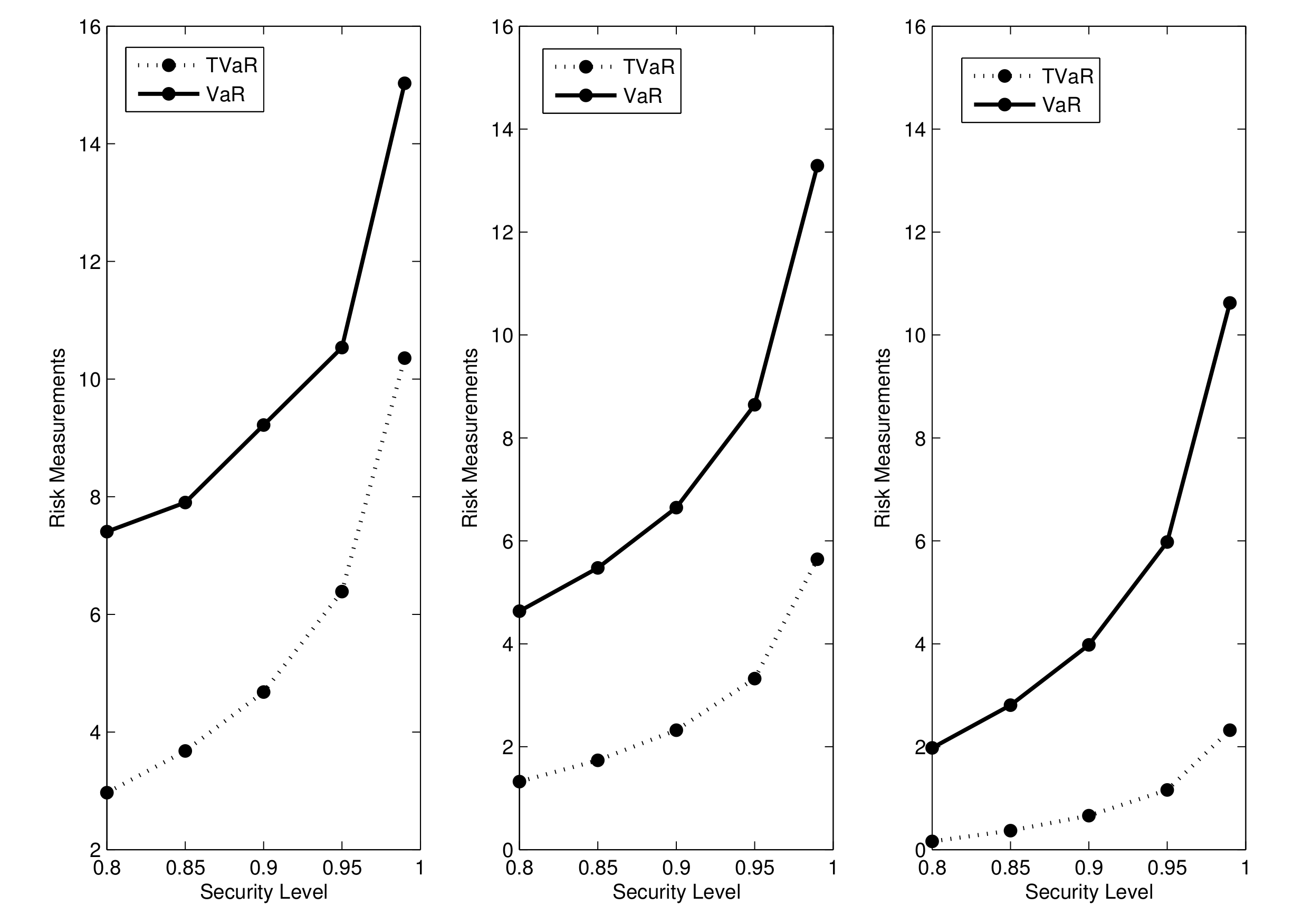
3.1. VaR Measure
3.2. TVaR Measure
4. Estimation
4.1. Maximum Likelihood
4.2. Moments
4.3. Proportions
4.4. Ordinary and Weighted Least-Squares
4.5. Cramér-von Mises
4.6. Right-Tail Anderson–Darling
4.7. Percentiles
5. Simulation Study
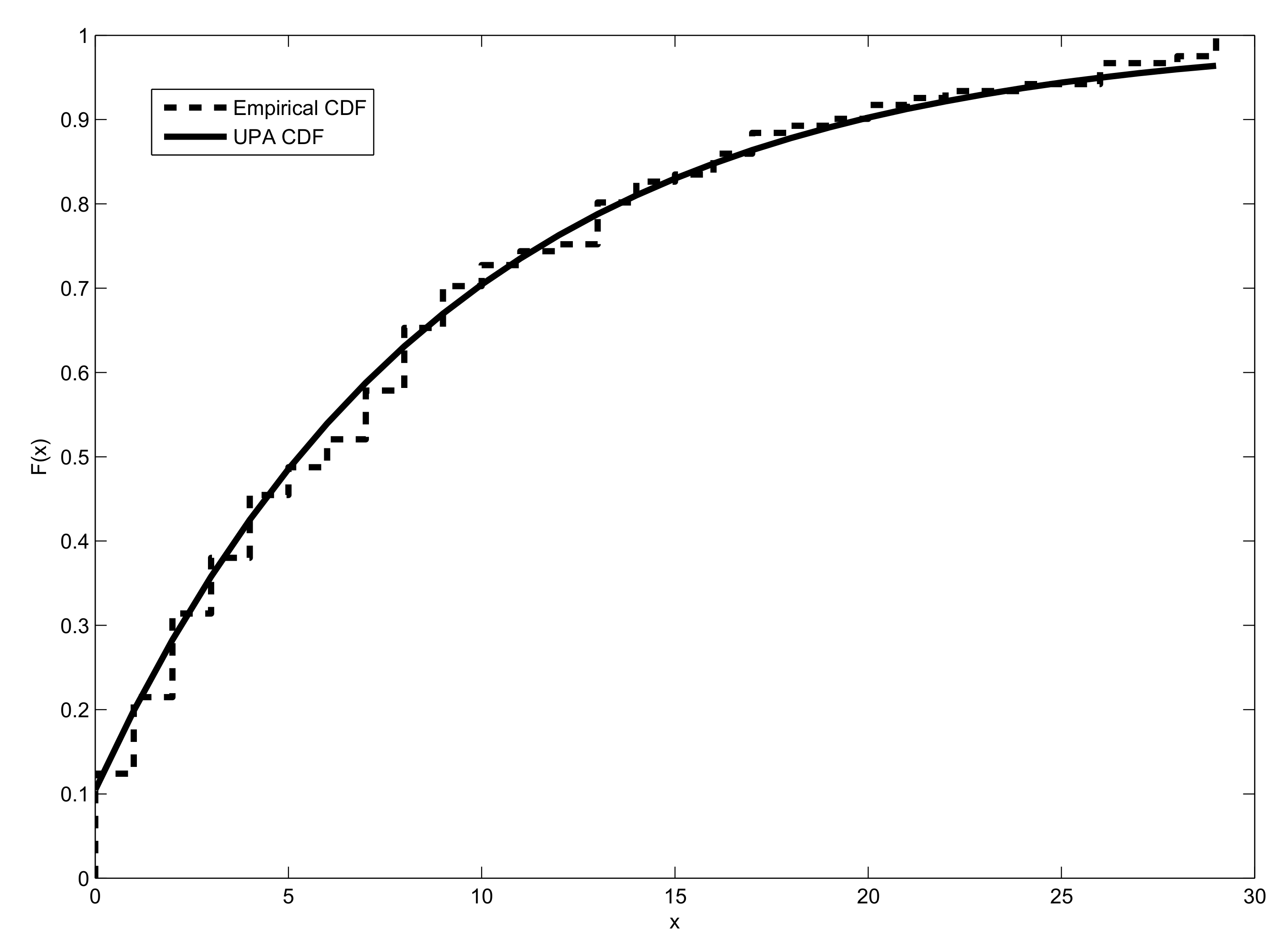
6. Modeling Biological Data
7. Conclusions
Author Contributions
Funding
Acknowledgments
Conflicts of Interest
References
- Nakagawa, T.; Osaki, S. Discrete Weibull distribution. IEEE Trans. Reliab. 1975, 24, 300–301. [Google Scholar] [CrossRef]
- Stein, W.E.; Dattero, R. A new discrete Weibull distribution. IEEE Trans. Reliab. 1984, 33, 196–197. [Google Scholar] [CrossRef]
- Roy, D. The discrete normal distribution. Commun. Stat. Theory Methods 2003, 32, 1871–1883. [Google Scholar] [CrossRef]
- Roy, D. Discrete Rayleigh distribution. IEEE Trans. Reliab. 2004, 53, 255–260. [Google Scholar] [CrossRef]
- Krishna, H.; Pundir, P.S. Discrete Burr and discrete Pareto distributions. Stat. Methodol. 2009, 6, 177–188. [Google Scholar] [CrossRef]
- Chakaraborty, S.; Chakaraborty, D. Discrete gamma distribution: Properties and parameter estimation. Commun. Stat. Theory Methods 2012, 41, 3301–3324. [Google Scholar] [CrossRef]
- Noughabi, M.S.; Rezaei, R.A.H.; Mohtashami, B.G.R. Some discrete lifetime distributions with bathtub-shaped hazard rate functions. Qual. Eng. 2013, 25, 225–236. [Google Scholar] [CrossRef]
- Al-Babtain, A.A.; Ahmed, A.H.N.; Afify, A.Z. A new discrete analog of the continuous Lindley distribution, with reliability applications. Entropy 2020, 22, 603. [Google Scholar] [CrossRef]
- Almazah, M.M.A.; Alnssyan, B.; Ahmed, A.H.N.; Afify, A.Z. Reliability properties of the NDL family of discrete distributions with its inference. Mathematics 2021, 9, 1139. [Google Scholar] [CrossRef]
- Hu, Y.; Peng, X.; Li, T.; Guo, H. On the Poisson approximation to photon distribution for faint lasers. Phys. Lett. A 2007, 367, 173–176. [Google Scholar] [CrossRef] [Green Version]
- Gomez-Deniz, E. A new discrete distribution: Properties and applications in medical care. J. Appl. Stat. 2013, 40, 2760–2770. [Google Scholar] [CrossRef]
- Akdoğan, Y.; Kuş, C.; Asgharzadeh, A.; Kınacı, I.; Shafari, F. Uniform-geometric distribution. J. Stat. Comput. Simul. 2016, 86, 1754–1770. [Google Scholar] [CrossRef]
- Kuş, C.; Akdoğan, Y.; Asgharzadeh, A.; Kınacı, I.; Karakaya, K. Binomial discrete Lindley distribution. Commun. Fac. Sci. Univ. Ank. Ser. Math. Stat. 2018, 68, 401–411. [Google Scholar] [CrossRef]
- Lv, H.Q.; Gao, L.H.; Chen, C.L. Ailamujia distribution and its application in support ability data analysis. J. Acad. Armored Force Eng. 2002, 16, 48–52. [Google Scholar]
- Hassan, A.; Shalbaf, G.A.; Bilal, S.; Rashid, A. A new flexible discrete distribution with spplications to count data. J. Stat. Theory Appl. 2020, 19, 102–108. [Google Scholar]
- Shaked, M.; Shanthikumar, J.G. Stochastic Orders; Springer: New York, NY, USA, 2007. [Google Scholar]
- Khan, M.S.A.; Khalique, A.; Abouammoh, A.M. On estimating parameters in a discrete Weibull distribution. IEEE Trans. Reliab. 1989, 38, 348–350. [Google Scholar] [CrossRef]
- Cramér, H. On the composition of elementary errors. Scand. Actuar. J. 1928, 1, 141–180. [Google Scholar] [CrossRef]
- Von Mises, R.E. Wahrscheinlichkeit Statistik und Wahrheit; Springer: Basel, Switzerland, 1928. [Google Scholar]
- Luceño, A. Fitting the generalized Pareto distribution to data using maximum goodness-of-fit estimators. Comput. Stat. Data Anal. 2006, 51, 904–917. [Google Scholar] [CrossRef]
- El-Morshedy, M.; Eliwa, M.S.; Altun, E. Discrete Burr-Hatke distribution with properties, estimation methods and regression model. IEEE Access 2020, 8, 74359–74370. [Google Scholar] [CrossRef]
- Sankaran, M. The discrete Poisson–Lindley distribution. Biometrics 1970, 26, 145–149. [Google Scholar] [CrossRef]
- Catheside, D.G.; Lea, D.E.; Thoday, J.M. Types of chromosome structural change induced by the irradiation of Tradescantia microspores. J. Genet. 1946, 47, 113–136. [Google Scholar] [CrossRef] [PubMed]


| Continuous Distribution | Discrete Distribution | Author |
|---|---|---|
| Weibull | Discrete Weibull | Nakagawa and Osaki [1] |
| Inverse Weibull | Discrete inverse Weibull | Stein and Dattero [2] |
| Normal and Rayleigh | Discrete normal and Rayleigh | Roy [3,4] |
| Burr XII and Pareto | Discrete Burr XII and Pareto | Krishna and Pundir [5] |
| Gamma | Discrete gamma | Chakraborty and Chakravarty [6] |
| Chen | Discrete Chen | Noughabi et al. [7] |
| Mean | B | ID | ||||
|---|---|---|---|---|---|---|
| 0.25 | 2.0000 | 6.0000 | 10.0000 | 74.0000 | 730.0000 | 3.0000 |
| 0.75 | 0.6667 | 1.1111 | 1.5555 | 5.1111 | 22.2963 | 1.6667 |
| 1.00 | 0.5000 | 0.7500 | 1.0000 | 2.7500 | 10.0000 | 1.5000 |
| 1.25 | 0.4000 | 0.5600 | 0.7200 | 1.7440 | 5.5584 | 1.4000 |
| 1.50 | 0.3333 | 0.4444 | 0.5555 | 1.2222 | 3.5185 | 1.3333 |
| 1.75 | 0.2857 | 0.3673 | 0.4490 | 0.9154 | 2.4281 | 1.2857 |
| 2.00 | 0.2500 | 0.3125 | 0.3750 | 0.7187 | 1.7812 | 1.2500 |
| 2.25 | 0.2222 | 0.2716 | 0.3210 | 0.5844 | 1.3672 | 1.2222 |
| 2.50 | 0.2000 | 0.2400 | 0.2800 | 0.4880 | 1.0864 | 1.2000 |
| 2.75 | 0.1818 | 0.2149 | 0.2479 | 0.4162 | 0.8872 | 1.1818 |
| 3.25 | 0.1538 | 0.1775 | 0.2011 | 0.3177 | 0.6297 | 1.1538 |
| 3.75 | 0.1333 | 0.1511 | 0.1689 | 0.2542 | 0.4751 | 1.1333 |
| 4.50 | 0.1111 | 0.1234 | 0.1358 | 0.1934 | 0.3370 | 1.1111 |
| 5.50 | 0.0909 | 0.0992 | 0.1074 | 0.1450 | 0.2353 | 1.0909 |
| 7.50 | 0.0667 | 0.0711 | 0.0755 | 0.0951 | 0.1400 | 1.0667 |
| 9.50 | 0.0526 | 0.0554 | 0.0582 | 0.0701 | 0.0968 | 1.0526 |
| 10.00 | 0.0500 | 0.0525 | 0.0550 | 0.0657 | 0.0896 | 1.0500 |
| 50.00 | 0.0100 | 0.0101 | 0.0102 | 0.0106 | 0.0114 | 1.0100 |
| 75.00 | 0.0067 | 0.0067 | 0.0067 | 0.0069 | 0.0073 | 1.0067 |
| 100.00 | 0.0050 | 0.0050 | 0.0050 | 0.0051 | 0.0053 | 1.0050 |
| 3.5 | 0.4306 | 7 | 0.2624 | ||
| 0.5 | 1.3863 | 4 | 0.3924 | 7.5 | 0.2494 |
| 1 | 0.9548 | 4.5 | 0.3612 | 8 | 0.2377 |
| 1.5 | 0.7498 | 5 | 0.3351 | 8.5 | 0.2272 |
| 2 | 0.6255 | 5.5 | 0.3129 | 9 | 0.2176 |
| 2.5 | 0.5407 | 6 | 0.2938 | 9.5 | 0.2090 |
| 3 | 0.4785 | 6.5 | 0.2771 | 10 | 0.2010 |
| Security Level | VaR | TVaR | ||||
|---|---|---|---|---|---|---|
| 0.25 | 0.80 | 2.9694 | 7.4074 | |||
| 0.85 | 3.6789 | 7.9012 | ||||
| 0.90 | 4.6789 | 9.2181 | ||||
| 0.95 | 6.3884 | 10.5350 | ||||
| 0.99 | 10.3577 | 15.0293 | ||||
| 0.5 | 0.80 | 1.3219 | 4.6338 | |||
| 0.85 | 1.7369 | 5.4739 | ||||
| 0.90 | 2.3219 | 6.6438 | ||||
| 0.95 | 3.3219 | 8.6438 | ||||
| 0.99 | 5.6438 | 13.2877 | ||||
| 1.5 | 0.80 | 0.1610 | 1.9772 | |||
| 0.85 | 0.3685 | 2.8073 | ||||
| 0.90 | 0.6610 | 3.9772 | ||||
| 0.95 | 1.1610 | 5.9772 | ||||
| 0.99 | 2.3219 | 10.6210 |
| n | MLE | POE | MOE | LSE | WLSE | CVME | RADE | PCE | |
|---|---|---|---|---|---|---|---|---|---|
| 30 | AVEs | 0.3571 | 0.3333 | 0.3571 | 0.3633 | 0.3635 | 0.3754 | 0.3742 | 0.3724 |
| MSEs | 0.3031 | 0.0076 | 0.0031 | 0.0039 | 0.0040 | 0.0205 | 0.0198 | 0.0764 | |
| ABSs | 0.0554 | 0.0875 | 0.0554 | 0.0626 | 0.0631 | 0.0863 | 0.0789 | 0.2624 | |
| MREs | 0.1583 | 0.2504 | 0.1583 | 0.1788 | 0.1804 | 0.2415 | 0.1428 | 0.8639 | |
| 75 | AVEs | 0.3505 | 0.3523 | 0.3505 | 0.3555 | 0.3557 | 0.3495 | 0.3465 | 0.3639 |
| MSEs | 0.0013 | 0.0027 | 0.0013 | 0.0017 | 0.0018 | 0.0101 | 0.0087 | 0.0458 | |
| ABSs | 0.0366 | 0.0521 | 0.0366 | 0.0415 | 0.0421 | 0.0774 | 0.0712 | 0.2139 | |
| MREs | 0.1046 | 0.1489 | 0.1046 | 0.1184 | 0.1204 | 0.2212 | 0.0712 | 0.6112 | |
| 100 | AVEs | 0.3521 | 0.3474 | 0.3521 | 0.3525 | 0.3521 | 0.3394 | 0.3416 | 0.3480 |
| MSEs | 0.0010 | 0.0019 | 0.0010 | 0.0013 | 0.0013 | 0.0057 | 0.0050 | 0.0065 | |
| ABSs | 0.0315 | 0.0435 | 0.0315 | 0.0355 | 0.0360 | 0.0602 | 0.0557 | 0.0634 | |
| MREs | 0.0901 | 0.1244 | 0.0908 | 0.1017 | 0.1029 | 0.1719 | 0.0557 | 0.1812 | |
| 150 | AVEs | 0.3505 | 0.3523 | 0.3505 | 0.3524 | 0.3524 | 0.3397 | 0.3403 | 0.3478 |
| MSEs | 0.0006 | 0.0018 | 0.0006 | 0.0008 | 0.0008 | 0.0045 | 0.0039 | 0.0049 | |
| ABSs | 0.0250 | 0.0428 | 0.0250 | 0.0291 | 0.0294 | 0.0537 | 0.0498 | 0.0556 | |
| MREs | 0.0714 | 0.1224 | 0.0714 | 0.0832 | 0.0841 | 0.1535 | 0.0498 | 0.1589 | |
| 200 | AVEs | 0.3509 | 0.3474 | 0.3508 | 0.3525 | 0.3525 | 0.3354 | 0.3389 | 0.3418 |
| MSEs | 0.0005 | 0.0012 | 0.0005 | 0.0006 | 0.0006 | 0.0023 | 0.0020 | 0.0024 | |
| ABSs | 0.0217 | 0.0349 | 0.0217 | 0.0247 | 0.0248 | 0.0392 | 0.0360 | 0.0393 | |
| MREs | 0.0621 | 0.0999 | 0.0621 | 0.0707 | 0.0710 | 0.1121 | 0.0360 | 0.1123 | |
| 300 | AVEs | 0.3505 | 0.3522 | 0.3505 | 0.3519 | 0.3516 | 0.3463 | 0.3465 | 0.3488 |
| MSEs | 0.0003 | 0.0007 | 0.0003 | 0.0004 | 0.0004 | 0.0010 | 0.0008 | 0.0009 | |
| ABSs | 0.0176 | 0.0272 | 0.0176 | 0.0203 | 0.0204 | 0.0261 | 0.0226 | 0.0236 | |
| MREs | 0.0504 | 0.0777 | 0.0504 | 0.0579 | 0.0583 | 0.0745 | 0.0226 | 0.0673 |
| n | MLE | POE | MOE | LSE | WLSE | CVME | RADE | PCE | |
|---|---|---|---|---|---|---|---|---|---|
| 30 | AVEs | 0.5172 | 0.5127 | 0.5172 | 0.5146 | 0.5155 | 0.4757 | 0.4785 | 0.4898 |
| MSEs | 0.0069 | 0.0138 | 0.0069 | 0.0089 | 0.0089 | 0.0167 | 0.0147 | 0.0217 | |
| ABBs | 0.0833 | 0.1176 | 0.0833 | 0.0943 | 0.0944 | 0.1028 | 0.0967 | 0.1136 | |
| MREs | 0.1667 | 0.2353 | 0.1667 | 0.1886 | 0.1888 | 0.2050 | 0.1934 | 0.2273 | |
| 75 | AVEs | 0.5145 | 0.4868 | 0.5145 | 0.5020 | 0.5016 | 0.4653 | 0.4713 | 0.4848 |
| MSEs | 0.0029 | 0.0051 | 0.0029 | 0.0037 | 0.0038 | 0.0073 | 0.0060 | 0.0077 | |
| ABBs | 0.0536 | 0.0714 | 0.0536 | 0.0612 | 0.0615 | 0.0703 | 0.0634 | 0.0704 | |
| MREs | 0.1071 | 0.1429 | 0.1071 | 0.1224 | 0.1230 | 0.1407 | 0.1267 | 0.1408 | |
| 100 | AVEs | 0.5126 | 0.4868 | 0.5127 | 0.5020 | 0.5016 | 0.4619 | 0.4588 | 0.4871 |
| MSEs | 0.0024 | 0.0041 | 0.0024 | 0.0029 | 0.0029 | 0.0056 | 0.0045 | 0.0059 | |
| ABBs | 0.0495 | 0.0638 | 0.0495 | 0.0542 | 0.0542 | 0.0620 | 0.0562 | 0.0615 | |
| MREs | 0.0989 | 0.1277 | 0.0989 | 0.1085 | 0.1085 | 0.1241 | 0.1124 | 0.1230 | |
| 150 | AVEs | 0.5098 | 0.5057 | 0.5097 | 0.5023 | 0.5019 | 0.4588 | 0.4678 | 0.4894 |
| MSEs | 0.0016 | 0.0032 | 0.0016 | 0.0020 | 0.0019 | 0.0045 | 0.0036 | 0.0040 | |
| ABBs | 0.0396 | 0.0563 | 0.0396 | 0.0447 | 0.0441 | 0.0562 | 0.0497 | 0.0508 | |
| MREs | 0.0791 | 0.1127 | 0.0791 | 0.0894 | 0.883 | 0.1124 | 0.0993 | 0.1016 | |
| 200 | AVEs | 0.5044 | 0.5005 | 0.5045 | 0.5011 | 0.5008 | 0.4600 | 0.4665 | 0.4906 |
| MSEs | 0.0011 | 0.0023 | 0.0011 | 0.0014 | 0.0014 | 0.0037 | 0.0030 | 0.0030 | |
| ABBs | 0.0327 | 0.0476 | 0.0327 | 0.0379 | 0.0379 | 0.0510 | 0.0456 | 0.0442 | |
| MREs | 0.0654 | 0.0952 | 0.0654 | 0.0755 | 0.0758 | 0.1021 | 0.0911 | 0.0883 | |
| 300 | AVEs | 0.5005 | 0.5004 | 0.5004 | 0.5003 | 0.5003 | 0.4573 | 0.4667 | 0.4914 |
| MSEs | 0.0008 | 0.0015 | 0.0008 | 0.0010 | 0.0010 | 0.0031 | 0.0024 | 0.0019 | |
| ABBs | 0.0282 | 0.0385 | 0.0282 | 0.0312 | 0.0315 | 0.0480 | 0.0406 | 0.0354 | |
| MREs | 0.0563 | 0.0769 | 0.0563 | 0.0625 | 0.0630 | 0.0961 | 0.0813 | 0.0708 |
| n | MLE | POE | MOE | LSE | WLSE | CVME | RADE | PCE | |
|---|---|---|---|---|---|---|---|---|---|
| 30 | AVEs | 1.5421 | 1.6429 | 1.5521 | 1.6069 | 1.6044 | 1.1887 | 1.2015 | 1.5306 |
| MSEs | 0.1406 | 0.2500 | 0.1406 | 0.2060 | 0.2029 | 0.2316 | 0.2203 | 1.0837 | |
| ABBs | 0.3750 | 0.5024 | 0.3750 | 0.4538 | 0.4504 | 0.4160 | 0.4045 | 0.4863 | |
| MREs | 0.2500 | 0.3333 | 0.2501 | 0.3025 | 0.3003 | 0.2773 | 0.2696 | 0.3241 | |
| 75 | AVEs | 1.5215 | 1.4737 | 1.5257 | 1.4992 | 1.4941 | 1.1389 | 1.1612 | 1.4721 |
| MSEs | 0.0428 | 0.0873 | 0.0428 | 0.0604 | 0.0617 | 0.1750 | 0.1594 | 0.1434 | |
| ABBs | 0.2069 | 0.2955 | 0.2069 | 0.2457 | 0.2483 | 0.3780 | 0.3598 | 0.2931 | |
| MREs | 0.1379 | 0.1970 | 0.1379 | 0.1638 | 0.1656 | 0.2520 | 0.2399 | 0.1954 | |
| 100 | AVEs | 1.5152 | 1.5247 | 1.5152 | 1.5029 | 1.5028 | 1.1337 | 1.1641 | 1.4760 |
| MSEs | 0.0475 | 0.0459 | 0.0475 | 0.0469 | 0.0470 | 0.1676 | 0.1450 | 0.1075 | |
| ABBs | 0.2179 | 0.2143 | 0.2179 | 0.2166 | 0.2169 | 0.3748 | 0.3471 | 0.2555 | |
| MREs | 0.1453 | 0.1429 | 0.1453 | 0.1444 | 0.1446 | 0.2499 | 0.2314 | 0.1703 | |
| 150 | AVEs | 1.5158 | 1.5270 | 1.5247 | 1.5110 | 1.5120 | 1.1305 | 1.1600 | 1.4791 |
| MSEs | 0.0278 | 0.0424 | 0.0278 | 0.0348 | 0.0347 | 0.1575 | 0.1364 | 0.0069 | |
| ABBs | 0.1667 | 0.2059 | 0.1667 | 0.1865 | 0.1862 | 0.3714 | 0.3431 | 0.2073 | |
| MREs | 0.1111 | 0.1373 | 0.1111 | 0.1243 | 0.1241 | 0.2476 | 0.2288 | 01382 | |
| 200 | AVEs | 1.5152 | 1.5123 | 1.5152 | 1.5000 | 1.4995 | 1.1211 | 1.1522 | 1.4794 |
| MSEs | 0.0221 | 0.0302 | 0.0220 | 0.0265 | 0.0265 | 0.1590 | 0.1306 | 0.0494 | |
| ABBs | 0.1486 | 0.1739 | 0.1486 | 0.1627 | 0.1629 | 0.3795 | 0.3479 | 0.1778 | |
| MREs | 0.0991 | 0.1159 | 0.0991 | 0.1084 | 0.1086 | 0.2530 | 0.2330 | 0.1186 | |
| 300 | AVEs | 1.5045 | 1.5057 | 1.5098 | 1.5032 | 1.5028 | 1.1205 | 1.1522 | 1.4813 |
| MSEs | 0.0127 | 0.0156 | 0.0127 | 0.0160 | 0.0159 | 0.1543 | 0.1306 | 0.0329 | |
| ABBs | 0.1129 | 0.1250 | 0.1129 | 0.1265 | 0.1260 | 0.3766 | 0.3479 | 0.1452 | |
| MREs | 0.0753 | 0.0833 | 0.0752 | 0.0844 | 0.0840 | 0.2531 | 0.2319 | 0.0968 |
| n | MLE | POE | MOE | LSE | WLSE | CVME | RADE | PCE | |
|---|---|---|---|---|---|---|---|---|---|
| 30 | AVEs | 3.4270 | 3.2500 | 3.2347 | 3.2366 | 3.2866 | 2.5001 | 2.5030 | 3.4441 |
| MSEs | 0.7347 | 1.0124 | 0.7347 | 1.0417 | 1.0248 | 1.5788 | 1.5904 | 1.8639 | |
| ABBs | 0.8571 | 1.0147 | 0.8571 | 1.0206 | 1.0123 | 1.1359 | 1.1275 | 1.4804 | |
| MREs | 0.2857 | 0.3333 | 0.2857 | 0.3402 | 0.3374 | 0.3786 | 0.3758 | 0.4935 | |
| 75 | AVEs | 3.1250 | 2.9091 | 3.1250 | 2.9339 | 2.9364 | 2.8859 | 2.9132 | 3.0907 |
| MSEs | 0.4307 | 0.4444 | 0.4307 | 0.4302 | 0.4304 | 1.4055 | 1.3384 | 1.2770 | |
| ABBs | 0.6562 | 0.6667 | 0.6563 | 0.6560 | 0.6561 | 1.1236 | 1.0963 | 0.7931 | |
| MREs | 0.2188 | 0.2222 | 0.2188 | 0.2187 | 0.2187 | 0.3745 | 0.3654 | 0.2644 | |
| 100 | AVEs | 3.1250 | 3.0714 | 3.1250 | 3.0711 | 3.0711 | 2.8642 | 2.8988 | 3.0839 |
| MSEs | 0.3265 | 0.3122 | 0.3265 | 0.3318 | 0.3289 | 1.4062 | 1.3243 | 0.8779 | |
| ABBs | 0.5714 | 0.5588 | 0.5714 | 0.5760 | 0.5735 | 1.1388 | 1.1045 | 0.6850 | |
| MREs | 0.1905 | 0.1863 | 0.1905 | 0.1920 | 0.1912 | 0.3796 | 0.3681 | 0.2283 | |
| 150 | AVEs | 3.0785 | 3.0714 | 3.0673 | 3.0650 | 3.0656 | 2.8513 | 2.8892 | 3.0408 |
| MSEs | 0.1712 | 0.2001 | 0.1712 | 0.2026 | 0.2031 | 1.3906 | 1.3021 | 0.5301 | |
| ABBs | 0.4138 | 0.4474 | 0.4138 | 0.4502 | 0.4507 | 1.1487 | 1.1109 | 0.5437 | |
| MREs | 0.1379 | 0.1491 | 0.1379 | 0.1500 | 0.1502 | 0.3829 | 0.3703 | 0.1819 | |
| 200 | AVEs | 3.0303 | 3.0714 | 3.0303 | 3.0578 | 3.0562 | 2.8470 | 2.8804 | 3.0547 |
| MSEs | 0.1357 | 0.1406 | 0.1357 | 0.1439 | 0.1449 | 1.3820 | 1.3047 | 0.3779 | |
| ABBs | 0.3684 | 0.3750 | 0.3684 | 0.3794 | 0.3807 | 1.1530 | 1.1197 | 0.4726 | |
| MREs | 0.1228 | 0.1250 | 0.1228 | 0.1265 | 0.1269 | 0.3844 | 0.3732 | 0.1576 | |
| 300 | AVEs | 3.0159 | 2.9884 | 3.0158 | 2.9923 | 2.9917 | 2.8412 | 2.8765 | 3.0507 |
| MSEs | 0.1033 | 0.1198 | 0.1033 | 0.1178 | 0.1183 | 1.3785 | 1.2945 | 0.2502 | |
| ABBs | 0.3214 | 0.3462 | 0.3214 | 0.3432 | 0.3439 | 1.1588 | 1.1235 | 0.3854 | |
| MREs | 0.1071 | 0.1154 | 0.1071 | 0.1144 | 0.1146 | 0.3863 | 0.3745 | 0.1285 |
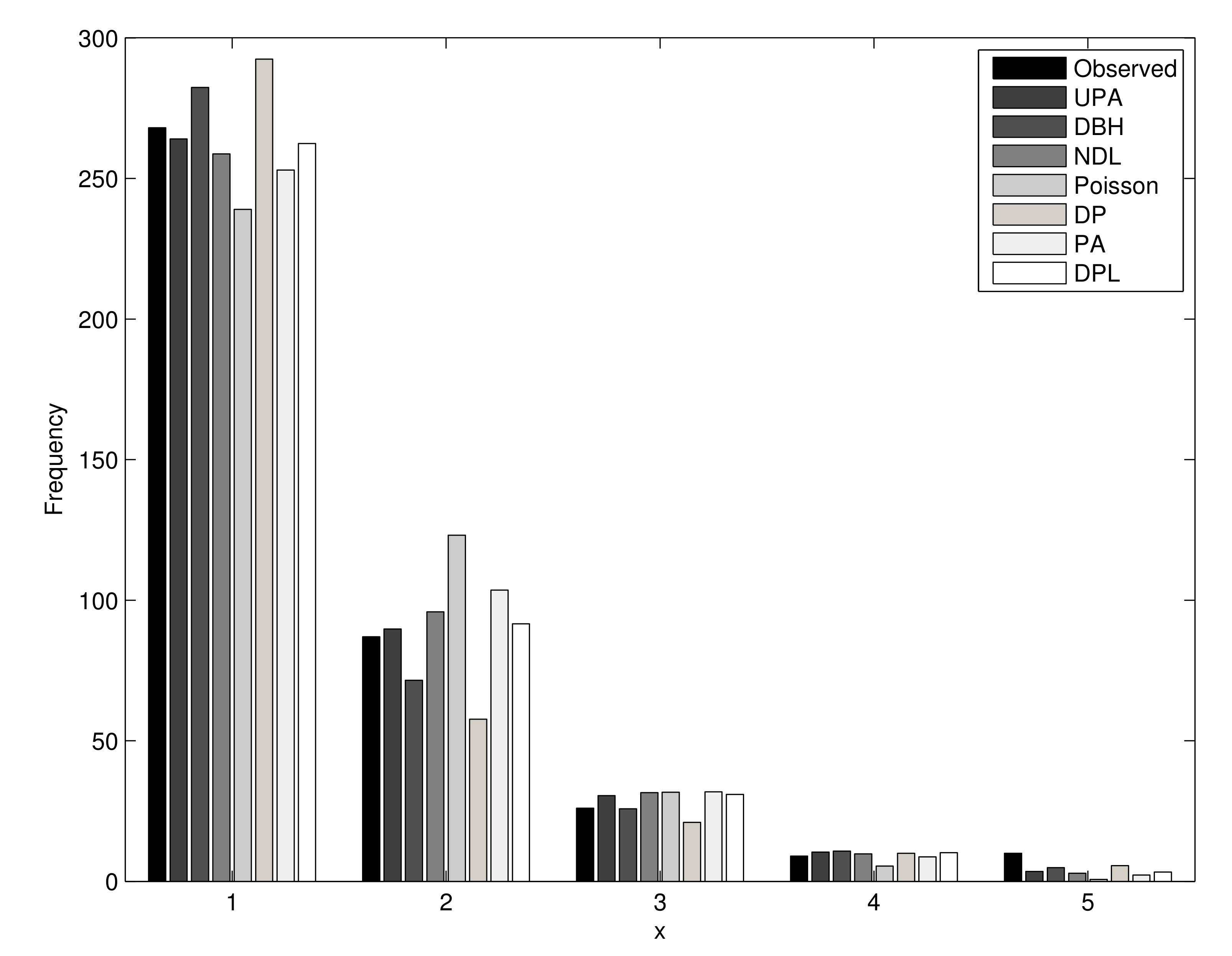
| Count | Observed | Expected | ||||||
|---|---|---|---|---|---|---|---|---|
| UPA | DBH | NDL | Poisson | Pareto | PA | DPL | ||
| 0 | 268 | 264.03 | 282.33 | 258.76 | 238.99 | 292.41 | 252.96 | 262.44 |
| 1 | 87 | 89.75 | 71.52 | 95.87 | 123.09 | 57.68 | 103.60 | 91.61 |
| 2 | 26 | 30.51 | 25.79 | 31.57 | 31.70 | 20.97 | 31.82 | 30.92 |
| 3 | 9 | 10.37 | 10.78 | 9.75 | 5.44 | 9.98 | 8.69 | 10.19 |
| 4 | 10 | 3.53 | 4.89 | 2.89 | 0.70 | 5.54 | 2.22 | 3.30 |
| Total | 400 | |||||||
| Parameters | 0.9709 | 0.5883 | 0.7530 | 0.5150 | 0.1504 | 1.9417 | 2.5012 | |
| 5.33 | 6.49 | 7.54 | 29.41 | 15.17 | 11.37 | 5.94 | ||
| 388.44 | 389.76 | 390.99 | 408.63 | 405.12 | 392.55 | 388.74 | ||
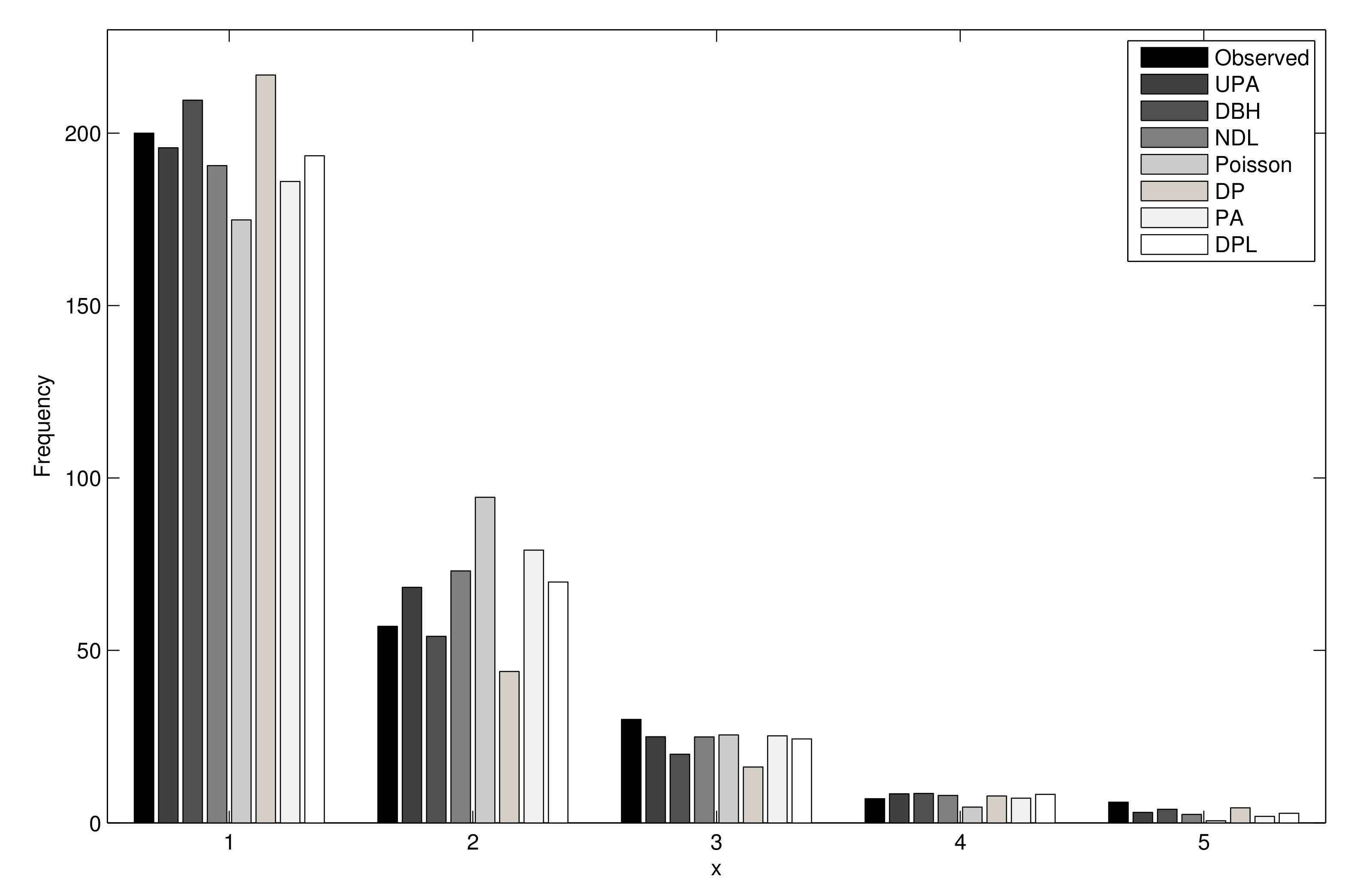
| Count | Observed | Expected | ||||||
|---|---|---|---|---|---|---|---|---|
| UPA | DBH | NDL | Poisson | Pareto | PA | DPL | ||
| 0 | 200 | 195.80 | 209.55 | 190.60 | 174.83 | 216.88 | 186.00 | 193.45 |
| 1 | 57 | 68.31 | 54.09 | 73.07 | 94.40 | 43.89 | 79.09 | 69.82 |
| 2 | 30 | 24.96 | 19.92 | 24.90 | 25.49 | 16.20 | 25.22 | 24.34 |
| 3 | 7 | 8.41 | 8.51 | 7.96 | 4.59 | 7.80 | 7.15 | 8.28 |
| 4≥ | 6 | 3.06 | 3.95 | 2.44 | 0.62 | 4.37 | 1.90 | 2.76 |
| Total | 300 | |||||||
| Parameters | 0.9259 | 0.6030 | 0.7444 | 0.5400 | 0.1570 | 1.8518 | 2.4002 | |
| 4.90 | 5.02 | 8.08 | 34.04 | 11.32 | 13.10 | 6.15 | ||
| 299.31 | 301.70 | 300.16 | 314.23 | 312.94 | 302.41 | 302.41 | ||
| Model | ||||
|---|---|---|---|---|
| UPA | 0.0585 | 757.2386 | 757.3214 | 377.6193 |
| DPL | 0.2318 | 765.8140 | 765.8968 | 381.9070 |
| NDL | 0.1901 | 767.1740 | 767.2568 | 382.5870 |
| PA | 0.1275 | 778.3318 | 778.4146 | 388.1659 |
| DP | 0.5857 | 849.9678 | 850.0506 | 423.9839 |
| DBH | 0.9920 | 909.8294 | 910.0438 | 452.9147 |
| Poisson | 7.8430 | 1260.3650 | 1260.4478 | 629.1825 |
Publisher’s Note: MDPI stays neutral with regard to jurisdictional claims in published maps and institutional affiliations. |
© 2021 by the authors. Licensee MDPI, Basel, Switzerland. This article is an open access article distributed under the terms and conditions of the Creative Commons Attribution (CC BY) license (https://creativecommons.org/licenses/by/4.0/).
Share and Cite
Aljohani, H.M.; Akdoğan, Y.; Cordeiro, G.M.; Afify, A.Z. The Uniform Poisson–Ailamujia Distribution: Actuarial Measures and Applications in Biological Science. Symmetry 2021, 13, 1258. https://doi.org/10.3390/sym13071258
Aljohani HM, Akdoğan Y, Cordeiro GM, Afify AZ. The Uniform Poisson–Ailamujia Distribution: Actuarial Measures and Applications in Biological Science. Symmetry. 2021; 13(7):1258. https://doi.org/10.3390/sym13071258
Chicago/Turabian StyleAljohani, Hassan M., Yunus Akdoğan, Gauss M. Cordeiro, and Ahmed Z. Afify. 2021. "The Uniform Poisson–Ailamujia Distribution: Actuarial Measures and Applications in Biological Science" Symmetry 13, no. 7: 1258. https://doi.org/10.3390/sym13071258
APA StyleAljohani, H. M., Akdoğan, Y., Cordeiro, G. M., & Afify, A. Z. (2021). The Uniform Poisson–Ailamujia Distribution: Actuarial Measures and Applications in Biological Science. Symmetry, 13(7), 1258. https://doi.org/10.3390/sym13071258