Dynamics of Fuzzy-Rough Cognitive Networks

Abstract

Fuzzy-rough cognitive networks (FRCNs) are interpretable recurrent neural networks, primarily designed for solving classification problems. Their structure is simple and transparent, while the performance is comparable to the well-known black-box classifiers. Although there are many applications on fuzzy cognitive maps and recently for FRCNS, only a very limited number of studies discuss the theoretical issues of these models. In this paper, we examine the behaviour of FRCNs viewing them as discrete dynamical systems. It will be shown that their mathematical properties highly depend on the size of the network, i.e., there are structural differences between the long-term behaviour of FRCN models of different size, which may influence the performance of these modelling tools.

1. Introduction

Artificial Intelligence (AI) models and methods are parts of our lives. However, most of the AI techniques are blackboxes in the sense, that they do not explain how and why they arrived at a specific conclusion. Explainable AI try to overcome this situation, developing models with interpretable semantics and transparency [1,2]. Fuzzy Cognitive Maps (FCMs) are one of the earliest EAI models, introduced by B. Kosko [3]. FCMs are recurrent neural networks employing weighted causal relation between the model’s concepts. Due to their modelling ability and interpretability, these models have a wide range of application [4,5].

Although FCMs have an enormous number of applications, only a few studies are devoted to the analytical and not empirical discussion of their behaviour. Boutalis et al. [6] examined the existence and uniqueness of fixed points of FCMs. Lee and Kwon studied the stability of FCMs using Lyapunov method [7]. Knight et al. [8] analyzed FCMs with linear and sigmoid transfer functions. In [9], the authors generalized the findings of [6] to FCMs with arbitrary sigmoid function. All of these studies arrived to the conclusion (although in a different form) that when the parameter of the sigmoid threshold function is small enough, then the FCM converges to a unique fixed point, regardless of the initial activation values.

The hybridisation of rough set theory and fuzzy set theory [10,11] provide a not only promising, but fruitful combination of different methods of handling and modelling uncertainty [12,13].

The application areas encompass a wide variety of sciences, so only a few of them are mentioned here, without the need for completeness. Fuzzy rough sets and fuzzy rough neural networks have been applied in feature selection problems [14], evolutionary fuzzy rough neural networks have been developed for stock prediction [15]. Fuzzy rough set models are used in multi-criteria decision-making in [16]. Classification tasks have been solved by fuzzy rough granular neural networks in [17]. The combination of unsupervised convolutional neural networks and fuzzy-rough C-mean was used effectively for clustering of large-scale image dataset in [18]. The environmental impact of a renewable energy system was estimated using fuzzy rough sets in [19]. The interval-valued fuzzy-rough based Delphi method was applied for evaluating the siting criteria of offshore wind farms in [20]. Another current direction is the fusion of neutrosophic theory and rough set theory [21]. An example of its application is the emission-based prioritization of bridge maintenance projects [22]. Nevertheless, in the aspect of this paper, fuzzy rough granular networks [23] are the most exciting applications of the synergy of fuzzy and rough theories.

Granular Computing [24] uses information granules, such as classes, clusters, subsets etc., just like humans do. Granular Neural Networks (GNNs) [25] make a synergy between the celebrated neural networks and granular computing [26]. Rough Cognitive Networks (RCN) are GNNs, introduced by Nápoles et al. [27], combining the abstract semantic of the three-way decision model with the neural reasoning mechanism of Fuzzy Cognitive Maps for addressing numerical decision-making problems. The information space is discretized (granulated) by using Rough Set Theory [28,29], which has many other interesting applications [30,31,32,33]. According to simulation results, RNN was capable to outperform standard classifiers. On the other hand, learning the similarity threshold parameter had significant computational cost.

Rough Cognitive Ensembles (RCEs) was proposed to overcome this computational burden [34]. It employs a collection of Rough Cognitive Networks as base classifiers, each operating at a different granularity level. This allows suppressing the requirement of learning a similarity threshold. Nevertheless, this model is still very sensitive to the similarity threshold upon which the rough information granules are built.

Fuzzy-Rough Cognitive Maps (FRCNs) has been introduced by Nápoles et al. [35]. The main feature of FRCNs is that the crisp information granules are replaced with fuzzy-rough granules. Based on simulation results, FRCNs show performance comparable to the best blackbox classifiers.

Vanloffelt et al. [36] studied the contributions of building blocks to the FRCNs’ performance via empirical simulations with several different network topologies. They concluded that the connections between positive neurons might not necessary to maintain the performance of FRCNs. The theoretical study by Concepción et al. [37] discussed the contribution of negative and boundary neurons. Moreover, they arrived at the conclusion that negative neurons have no impact on the decision, and the ranking between positive neuron remains invariant during the whole reasoning process.

Besides the results presented in [37], this paper was motivated by the fact that only a few studies are discussing the behaviour of cognitive networks from the strict mathematical point of view. Nevertheless, such studies may provide us with information about what we can or cannot achieve with these models. Analyzing the behaviour and contribution of the building blocks unveils the exact role of components of the complex structure: which part is crucial and which one is unnecessary etc. In this paper, we do not develop, neither implement another new fuzzy-rough model. Instead, we analyze the behaviour of FRCNs, which are comparable in performance to the best black-box classifiers. Because of their proven competitiveness [35], there is no need for further model verification and validation.

In the current paper, the dynamical behaviour of fuzzy-rough cognitive networks is examined. The main contributions are the following: first, we show that stable positive neurons have at most two different activation values for any initial activation vectors. Then we show that a certain point with equal coordinates (called trivial fixed point) is always a fixed point, nevertheless, not always a fixed point attractor. Furthermore, a condition for the existence of a unique, globally attractive fixed point is also stated. Complete analysis of the dynamics of positive neurons for two and three decision classes is provided. Finally, we show that for a higher number of classes, the occurrence of limit cycles is a necessity and the vast majority of initial activation values lead to oscillation. The rest of the paper is organized as follows. In Section 2, we recall the construction of fuzzy-rough cognitive maps and overview the existing results about their behaviour. In Section 3, a summary of the mathematical background necessary for further investigation of the dynamics of FRCNs is provided, including contraction mapping and elements of bifurcation theory. Section 4 presents general result about the dynamics of positive neurons, condition for unique fixed point attractor and refinement of some findings of [37]. Section 5 introduces size-specific results for FRCNs, providing a complete description for the case of two and three decision classes and pointing out that over a specific size, oscillation behaviour will be naturally present. Section 6 discusses the relation of the behaviour of positive neurons to the final decision class of FRCNs. The paper ends with a short conclusion in Section 7.

2. Fuzzy-Rough Cognitive Networks

In this section, we shortly summarize the basic notions of fuzzy-rough cognitive networks and the findings about their dynamical properties reported in the literature. It is based on the works [35,36,37].

2.1. Construction of FRCNs

Building up FRCNs includes the following three steps: information space granulation, network construction and finally, network exploitation.

Information space granulation means dividing available information into granules. Let $\mathcal{U}$ denote the universe of discourse and $X=\{X_1,\dots ,X_N\}$, $X\subset \mathcal{U}$. Then $X_c\subset \mathcal{U}$ is the subset containing all objects assigned (labelled) to decision class $D_c$. The membership degree of $x\in \mathcal{U}$ to $X_c$ is computed in a binary way:

$${\mu }_{X_c}\left(x\right)=\left\{\begin{array}{cc}1\hfill & ,x\in X_c\hfill \\ 0\hfill & ,x\notin X_c\hfill \end{array}\right..$$

(1)

Membership function ${\mu }_P(y,x)$ is the next component, using similiraty degree between two instances x and y:

$${\mu }_P(y,x)={\mu }_{X_c}\left(x\right)\phi (x,y)={\mu }_{X_c}\left(x\right)(1-\delta (x,y)),$$

(2)

where ${\mu }_P:U\times U\to [0,1]$ is the membership degree of y to $X_c$, given that x belongs to $X_c$ (in this sense, it is a conditional membership degree). It is composed by the previously defined binary membership function ${\mu }_{X_c}\left(x\right)$ and the similarity degree $\phi (x,y)$. The later is based on a normalized distance measure $\delta (x,y)$. Membership functions for the lower and upper approximation for any fuzzy set $X_c$, respectively:

$$\begin{array}{cc}\hfill {\mu }_{P_{\ast }\left(X_c\right)}\left(x\right)& =\min \left\{{\mu }_{X_c}\left(x\right),\underset{y\in \mathcal{U}}{\inf }\mathcal{I}({\mu }_P(y,x),{\mu }_{X_c}\left(x\right))\right\},\hfill \end{array}$$

(3)

$$\begin{array}{cc}\hfill {\mu }_{P^{\ast }\left(X_c\right)}\left(x\right)& =\max \left\{{\mu }_{X_c}\left(x\right),\underset{y\in \mathcal{U}}{\sup }\mathcal{T}({\mu }_P(y,x),{\mu }_{X_c}\left(x\right))\right\}.\hfill \end{array}$$

(4)

Here $\mathcal{I}$ denotes an implication function and $\mathcal{T}$ denotes a conjunction function. As a next step, we calculate the membership functions associated to the positive, negative and boundary regions:

$$\begin{array}{cc}\hfill {\mu }_{POS\left(X_c\right)}\left(x\right)& ={\mu }_{P_{\ast }\left(X_c\right)}\left(x\right),\hfill \end{array}$$

(5)

$$\begin{array}{cc}\hfill {\mu }_{NEG\left(X_c\right)}\left(x\right)& =1-{\mu }_{P^{\ast }\left(X_c\right)}\left(x\right),\hfill \end{array}$$

(6)

$$\begin{array}{cc}\hfill {\mu }_{BND\left(X_c\right)}\left(x\right)& ={\mu }_{P^{\ast }\left(X_c\right)}\left(x\right)-{\mu }_{P_{\ast }\left(X_c\right)}\left(x\right).\hfill \end{array}$$

(7)

After determining the membership functions of the decision classes, we construct a network using four type of neurons:

• $\mathcal{D}=\{D_1,\dots ,D_N\}$ is the set of decision neurons,
• $\mathcal{P}=\{P_1,\dots ,P_N\}$ is the set of positive neurons,
• $\mathcal{N}=\{N_1,\dots ,N_N\}$ is the set of negative neurons,
• $\mathcal{B}=\{B_1,\dots ,B_N\}$ is the set of boundary neurons.

The recurrent neural network have N output neurons (decision neurons). The number of input neuron is between $2N$ and $3N$, depending on the number of non-empty boundary regions. The ‘wiring’ between the neurons is based on the following steps (see Algorithm 1). Positive, negative and boundary neurons influence themselves with intensity 1. Each positive neuron influence the decision neuron related to it with intensity 1, moreover these neurons act on the other positive and decision neurons with intensity $-1$. Finally, if two decision classes share non-empty boundary regions, then each boundary neuron influences both decision neurons with intensity 0.5. As it is clear from this setting, the weights of a FRCN are not determined by learning methods, they are based on the semantic relations between the information granules.

Algorithm 1: The construction procedure of the fuzzy-rough cognitive network.

The computation of initial activation values ($A_i^{\left(0\right)}$s) of the neurons is based in the similiraty degree between the new object y and all $x\in \mathcal{U}$, and the membership degree of every x to positive, negative and boundary regions. The initial activation value of decision neurons is zero.

$$\begin{array}{ccc}\hfill & \mathrm{Positive} \mathrm{neurons} \left(P_i\right):\hfill & \hfill A_i^{\left(0\right)}=\frac{{\sum }_{x\in U}\mathcal{T}(\phi (x,y),{\mu }_{POS\left(X_c\right)}\left(x\right))}{{\sum }_{x\in U}{\mu }_{POS\left(X_c\right)}\left(x\right)}\end{array}$$

(8)

$$\begin{array}{ccc}\hfill & \mathrm{Negative} \mathrm{neurons} \left(N_i\right):\hfill & \hfill A_i^{\left(0\right)}=\frac{{\sum }_{x\in U}\mathcal{T}(\phi (x,y),{\mu }_{NEG\left(X_c\right)}\left(x\right))}{{\sum }_{x\in U}{\mu }_{NEG\left(X_c\right)}\left(x\right)}\end{array}$$

(9)

$$\begin{array}{ccc}\hfill & \mathrm{Boundary} \mathrm{neurons} \left(B_i\right):\hfill & \hfill A_i^{\left(0\right)}=\frac{{\sum }_{x\in U}\mathcal{T}(\phi (x,y),{\mu }_{BND\left(X_c\right)}\left(x\right))}{{\sum }_{x\in U}{\mu }_{BND\left(X_c\right)}\left(x\right)}\end{array}$$

(10)

After determining the initial values, the next step is network exploitation, by the iteration rule

$$A_i^{(t+1)}=f\left(\sum _{j=1}^N{w}_{ij}{A}_j^{\left(t\right)}\right).$$

(11)

or in matrix vector form $A^{(t+1)}=f(W{A}^{\left(t\right)})$, where f is understood coordinate-wise. Here $w_{ij}$ is the weight of the connection from neuron $C_j$ to neuron $C_i$. Function $f\left(x\right)=\frac{1}{1+e^{-\lambda x}}$ keeps the values in the $(0,1)$ range. For high $\lambda$ values, $f\left(x\right)$ tends to behave like the step function, while for very small $\lambda$ values, the activation values converge to a unique fixed point attractor, regardless of the initial activation values, producing the same output for every input values. The $\lambda =5$ choice is widely used in FCM applications, FRCNs employ this parameter value, too. The iteration stops when

• activation values converge to a fixed point attractor (practically it means that the consecutive values do not show reasonable change ), or
• a predefined maximal number of iteration is reached.

Finally, the label of the decision neuron with highest activation value is assigned the classified object. Figure 1 shows the FRCN’s structure for a binary classification problem.

2.2. Preliminary Results on the Dynamics of FRCNs

In this subsection, we shortly summarize the main contributions of [37] regarding the dynamics of fuzzy-rough cognitive networks. For detailed explanations and proofs, see [37].

• Negative and boundary neurons always converge to a unique fixed value. This value depends on parameter $\lambda$, but the convergence and uniqueness are independent of $\lambda$.
• The ranking between positive neurons remains invariant during the recurrent reasoning. As we will see in Section 5, although this statement is absolutely true in the strict mathematical sense, from the practical point if view, in some cases it has very limited applicability.
• In an FRCN with N decision classes, there will always be $N-1$ positive neurons with activation values less than or equal to $1/2$ (after at least one iteration step).
• In an FRCN there will be at most one neuron with activation value higher or equal to $1/2$ (after at least one iteration step).

Consider the updating rule $A_i^{(t+1)}=f\left({\sum }_{j=1}^N{w}_{ij}{A}_j^{\left(t\right)}\right)$ (see Equation (11)), where f is the sigmoid function with parameter $\lambda$. Assuming that positive neurons reach stable states, for every i it holds, that $P_i^{(t+1)}=P_i^{\left(t\right)}=f\left({\sum }_{j=1}^N{w}_{ij}{P}_j^{\left(t\right)}\right)$. Recall that each positive neuron is influenced by the other positive neurons with weight $-1$, while influences itself with weight 1 (i.e., if $i=j$, then $w_{ij}=1$, otherwise $w_{ij}=-1$). Consequently, we have

$$P_i^{\left(t\right)}=P_i^{(t+1)}=\frac{1}{1+e^{-\lambda \left(P_i^{\left(t\right)}-{\displaystyle \sum _{j=1,j\ne i}^N}{P}_j^{\left(t\right)}\right)}}=\frac{1}{1+e^{-\lambda \left(2P_i^{\left(t\right)}-{\displaystyle \sum _{j=1}^N}{P}_j^{\left(t\right)}\right)}}.$$

(12)

Now let us further investigate the equation ${\displaystyle P_i^{\left(t\right)}=\frac{1}{1+e^{-\lambda \left(2P_i^{\left(t\right)}-{\displaystyle \sum _{j=1}^N}{P}_j^{\left(t\right)}\right)}}}$. Expressing ${\displaystyle \sum _{j=1}^N}{P}_j^{\left(t\right)}$ we get the following equation:

$$\sum _{j=1}^N{P}_j^{\left(t\right)}=\frac{1}{\lambda }\ln \frac{1-P_i^{\left(t\right)}}{P_i^{\left(t\right)}}+2P_i^{\left(t\right)},$$

(13)

on the left hand side we find the sum of all activation values, which depends on the value of $P_i^{\left(t\right)}$ (recall that $P_i^{\left(t\right)}$ is the stabilized activation value of any positive neuron). The sum of the activation values is a function of $P_i^{\left(t\right)}$, of course. Define the following real function:

$$s\left(x\right)=\frac{1}{\lambda }\ln \frac{1-x}{x}+2x.$$

(14)

From the behaviour of $s\left(x\right)$, the authors derived some properties of the positive neurons:

• If $\lambda \le 2$, then $s\left(x\right)$ is monotone decreasing, thus a specific value can be produced by a single input value x. It means that if $\lambda \le 2$ and the positive neurons are stable (converge to a fixed point), then they have the same activation value.
• If $\lambda >2$, then $s\left(x\right)$ produces the same value for at most three different input values in $(0,1)$. It means that if the vector of positive neurons converges to a fixed point, then this vector has at most three different coordinate values.

In Section 4 and Section 5, we refine these statements and introduce some additional results regarding the dynamics of FRCNs.

3. Mathematical Background

The updating rule of FRCNs suggest to handle them as discrete dynamical systems. In this section, we briefly summarize the most important notions and methods used in the forthcoming sections.

3.1. Contraction Mapping

In the network exploitation phase, we apply the iteration rule Equation (11) again and again until the activation values stabilize (or the number of iterations reaches the predefined maximum). If the activation values stabilize (i.e., arrive an equilibrium state), then the difference between the outputs of two consecutive iteration steps will be smaller and smaller. In other words, the iteration contracts a subset of the state space (or the whole state space) into a single point. The following definition provides a strict mathematical description of this property.

Definition 1

(see [38], p. 220). Let $(X,d)$ be a metric space, with metric d. If φ maps X into X and if there is a number $c<1$ such that

$$d\left(\phi \left(x\right),\phi \left(y\right)\right)\le cd(x,y)$$

(15)

for all $x,y\in X$, then φ is said to be a contraction of X into X.

If the iteration reaches an equilibrium state, then this state will not change by applying the updating rule. Mathematically speaking, it is a fixed point of the mapping generating the iteration. The following famous theorem establishes connection between the contraction mapping and a unique fixed point.

Theorem 1

(Contraction mapping theorem or Banach’s fixed point theorem, see [38], pp. 220–221). If X is a complete metric space, and if φ is a contraction of X into X, then there exists one and only one $x\in X$ such that $\phi \left(x\right)=x$.

The proof to this theorem is constructive (see [38], p. 221) and offers a straightforward way to find this unique fixed point. We only have to pick an arbitrary element of X and apply mapping $\phi$ again and again. The limit will be the unique fixed point of $\phi$: $x_n=\phi \left(x_{n-1}\right)$, then ${\lim }_{n\to \infty }{x}_n=x^{\ast }$ and $\phi \left(x^{\ast }\right)=x^{\ast }$.

An arbitrary fixed point $x^{\ast }$ is said to be asymptotically stable if starting the iteration close enough to $x^{\ast }$, the limit will be $x^{\ast }$. Moreover, the fixed point $x^{\ast }$ is said to be globally asymptotically stable if starting the iteration from any element of the state space, the limit will be $x^{\ast }$. Based on Theorem 1 and its constructive proof, it is clear that the unique fixed point of a contraction is globally asymptotically stable.

3.2. Elements of Bifurcation Theory

The dynamics of a discrete dynamical system may change, if its parameters are varied. A qualitative change of the dynamical behaviour, e.g., a transition from a unique stable fixed point to multiple fixed points or oscillation, is called bifurcation and the corresponding critical parameter is called bifurcation point.

The detailed description of the dynamics of FRCNs requires the application of the elements of bifurctaion theory. Here only the most important notions are listed. For more details, see [39,40].

Consider a discrete-time dynamical system depending on only one parameter $\lambda$ ($G:{\mathbb{R}}^n\to {\mathbb{R}}^n$):

$$x_{k+1}=G(x_k,\lambda ),x_k\in {\mathbb{R}}^n,\lambda \in \mathbb{R},$$

(16)

where function G is smooth with respect to x and $\lambda$. Let’s assume that $x_0$ is a fixed point of the mapping with parameter ${\lambda }_0$. The local stability (resistance agianst small perturbations) of the fixed point depends on the eigenvalues of the Jacobian evaluated at $x_0$ ($J_G\left(x_0\right)$). If the Jacobian has no eigenvalues on the unit circle, $x_0$ is said to be hyperbolic. Hyperbolic fixed points can be categorized according to the eigenvalues of $J_G\left(x_0\right)$:

• If all of the eigenvalues lie inside the unit circle (i.e., the absolute value of the eigenvalues is less than one), then it is an asymptotically stable fixed point. In other words, this fixed point attracts the space in every direction in its (sometimes very small) neighborhood. Consequently, its basin of attraction is an n dimensional subset of then n dimensional space.
• If there are some eigenvalues (at least one) with absolute value greater than one, and there are some (at least one) eigenvalues with absolute value less than one, then it is a saddle point. It means that this fixed point may attract points of the space in some, but not every direction in its neighborhood. Consequently, the dimension of its basin of attraction is less than n.
• If all of the eigenvalues has absolute value greater than one, then it is an unstable fixed point (repeller fixed point).

In the FCM theory and similary in FRCN terminology, stable fixed point is a fixed point, that can be a limit of the iteration. In this sense, stable and saddle fixed points are considered as stable in the FCM (FRCN) sense. Nevertheless, their dynamical behavior could be very different. We will see in Section 5 that different type of fixed points have significantly different size of basin of attractions. In other words, some fixed points are less important than others.

The simplest ways the hyperbolicity can be violeted are the following:

• A simple positive eigenvalue crosses the unit circle at $\alpha =1$. The bifurcation associated to this scenario is called saddle-node bifurcation. It is a birth of new fixed points.
• A simple negative eigenvalue crosses the unit circle at $\alpha =-1$. This causes period-doubling bifurcation, the birth of limit cycles.
• A pair of complex conjugate eigenvalues approaches the unit circle at ${\alpha }_{1,2}=e^{i\varphi }$, $\varphi \in (0,\pi )$. This is the so-called Neimark-Sacker bifurcation, causes the occurence of a closed invariant curve.

It will be shown in Section 5, that depending on the size of the FRCN, different types of bifurcations determine the main dynamics of the system.

4. General Results on the Dynamics of Positive Neurons

In this section, we introduce some general results about the dynamics of positive neurons. Size specific results are presented in Section 5.

With start with the refinement of a result from [37]. Further investigation of the function $s\left(x\right)$ (see Equation (14)) provides more information about the possible fixed points of positive neurons (see Figure 2). It has been shown that there are at most one positive neuron with activation value higher than $1/2$. If $s\left(x\right)>1$, then a specific value may be produced by at most three different values of x. But two of these values are higher than $1/2$, thus only one of them get a role in the activation vector. It means that one coordinate of the activation vector is greater than $1/2$ and the remaining ones are less than $1/2$ and they have equal values.

Consider now the case, when $s\left(x\right)<1$. Observe that the graph of $s\left(x\right)$ is symmetrical about the point $(1/2,1)$ (it can be easily verified analytically). Let us choose a specific value $\gamma =s\left(x\right)$, such that the horizontal line $y=\gamma$ has three intersection points with the graph. Denote the first coordinates of theses point by $x_1,x_2,x_3$ ($x_1<x_2<x_3$). Using the symmetry of the function, we can conclude that $x_1>1-x_3$. Consequently, $x_1+x_3>1$. Since the sum of the activation values is less than 1 ($s\left(x\right)<1$), it follows that there can be at most two different values ($x_1$ and $x_2$) in the activation vector for any given $s\left(x\right)$.

Summarizing this short argument, if the activation vector of positive neurons converges to a fixed point, then it may have at most two different coordinate values.

The iteration rule for the updating of the neurons’ activation values has the form $A^{(t+1)}=f\left(W{A}^{\left(t\right)}\right),$ where the sigmoid is applied coordinate-wise and W is the connection matrix of the network. Based on the construction of the network (see Algorithm 1), it has the following block form:

$$W=\begin{array}{c}\mathrm{neuron}\mathrm{sets}\\ \mathcal{D}\\ \mathcal{B}\\ \mathcal{N}\\ \mathcal{P}\end{array}\begin{array}{c}\begin{array}{cccc}\mathcal{D}& \mathcal{B}& \mathcal{N}& \mathcal{P}\end{array}\\ \left[\begin{array}{cccc}O& W_B& -I& W_D\\ O& I& O& O\\ O& O& I& O\\ O& O& O& W_P\end{array}\right]\end{array},$$

(17)

where O, I denote zero matrix and identity matrix, respectively. $W_B$ describes the connections from boundary to decision neurons (it contains 0 s and 0.5 s, their positions depend on non-empty boundary regions), $W_P$ describes the connections between positive neurons (if $i=j$, then $w_{ij}=1$, else $w_{ij}=-1$), $W_D=W_P$ contains the connections from positive neurons to decision neurons.

Because of the upper-diagonal block structure, instead of dealing with the whole matrix, we can use the blocks. It has been proved in [37] that activation values of the negative and boundary neurons converge to the same unique value, which depends on $\lambda$, but independent of the initial activation values. Positive neurons influence themselves, each other and decision neurons, but do not receive input from other set of neurons. Their activation values are propagated to the decision neurons. In a long run, when neurons reach a stable state (or the iteration is stopped by achieving the maximal number of iterations), the propagated value is their stable (or final) state. In the following, we examine the long-term behaviour of positive neurons.

Lemma 1.

For every $\lambda >0$ and every number of decision classes N, there always exists a fixed point of the positive neurons, whose coordinates are the same. Nevertheless, this fixed point is not always a fixed point attractor.

Proof. 

Consider the fixed point equation for every $1\le j\le N$:

$$\begin{array}{cc}\hfill P& =f\left(W_{P}P\right)\hfill \end{array}$$

(18)

$$\begin{array}{cc}\hfill \left[\begin{array}{c}{P}_1\\ ⋮\\ P_N\end{array}\right]& =f\left(W_P\left[\begin{array}{c}{P}_1\\ ⋮\\ P_N\end{array}\right]\right)\hfill \end{array}$$

(19)

In coordinate-wise form:

$$P_j=\frac{1}{1+e^{-\lambda \left(P_j-{\displaystyle \sum _{i=1,j\ne j}}{P}_i\right)}}=\frac{1}{1+e^{-\lambda \left(2P_j-{\displaystyle \sum _{i=1}}{P}_i\right)}}$$

(20)

If $P_j=x$ for every $1\le j\le N$, then it simplifies to the following equation:

$$x=\frac{1}{1+e^{-\lambda \left(2-N\right)x}}=\frac{1}{1+e^{\lambda \left(N-2\right)x}}$$

(21)

We show that there always exists a unique solution to this equation. Let us introduce the function

$$g\left(x\right)=x-\frac{1}{1+e^{\lambda \left(N-2\right)x}}.$$

(22)

Function $g\left(x\right)$ is continuous and differentiable, moreover $g\left(0\right)=-0.5<0$ and $g\left(1\right)=1-\frac{1}{1+e^{\lambda \left(N-2\right)}}>0$, thus it has at least one zero in $(0,1)$. According to Rolle’s theorem, between two zeros of a differentiable function its derivative has a zero. The derivative is

$$g^{\prime }\left(x\right)=1+\frac{\lambda \left(N-2\right)e^{\lambda \left(N-2\right)x}}{{(1+e^{\lambda \left(N-2\right)x})}^2},$$

(23)

which is always positive. It means that there is exactly one zero of $g\left(x\right)$ in $(0,1)$. Consequently, we have shown that for any given $\lambda >0$ and N, there is exactly one fixed point of the positive neurons with equal coordinates. There may be other fixed points, but their coordinates are not all the same. □

The following lemma plays a crucial role in the proof of Theorem 2 and in the examination of the Jacobian of the iteration mapping.

Lemma 2.

Let $W_P$ be an $N\times N$ matrix with the following entries:

$$w_{ij}=\left\{\begin{array}{cc}1& \mathrm{if} i=j\hfill \\ -1& \mathrm{if} i\ne j\hfill \end{array}\right.$$

(24)

Then the eigenvalues of $W_P$ are $2-N$ (with multiplicity one) and 2 (with multiplicity $N-1$).

Proof. 

Basic linear algebra. □

Theorem 2.

Consider a fuzzy cognitive map (recurrent neural network) with sigmoid transfer function ($f\left(x\right)=1/(1+e^{-\lambda x})$) and with weight matrix $W_p$ whose entries are

$$w_{ij}=\left\{\begin{array}{cc}1& \mathrm{if} i=j\hfill \\ -1& \mathrm{if} i\ne j\hfill \end{array}\right.$$

(25)

If

$$\lambda <\frac{4}{\max \{2,|2-N\left|\right\}},$$

then it has exactly one fixed point. Moreover, this fixed point is a global attractor, i.e., the iteration starting from any initial activation vector ends at this point.

Proof. 

We are going to show that if the condition in theorem is fulfilled, then the mapping $P\to f\left(W_{P}P\right)$ is contraction, thus according to Banach’s theorem, it has exactly one fixed point and this fixed point is globally asymptotically stable, i.e., iterations starting from any initial vectors arrive to this fixed point. Let us choose two different initial vectors, P and $P^{\prime }$. Then

$$\begin{array}{cc}\hfill & \parallel f\left(W_{P}P\right)-f\left(W_P{P}^{\prime }\right){\parallel }_2={\left({\displaystyle \sum _{i=1}^N}{\left[f\left({\displaystyle \sum _{j=1}^N}{w}_{ij}{p}_j\right)-f\left({\displaystyle \sum _{j=1}^N}{w}_{ij}{p}_j^{\prime }\right)\right]}^2\right)}^{1/2}\hfill \end{array}$$

(26)

$$\begin{array}{cc}\hfill & \le {\left({\displaystyle \sum _{i=1}^N}{\left[\frac{\lambda }{4}\left({\displaystyle \sum _{j=1}^N}{w}_{ij}{p}_j-{\displaystyle \sum _{j=1}^N}{w}_{ij}{p}_j^{\prime }\right)\right]}^2\right)}^{1/2}=\frac{\lambda }{4}{\left({\displaystyle \sum _{i=1}^N}{\left[{\displaystyle \sum _{j=1}^N}{w}_{ij}(p_j-p_j^{\prime })\right]}^2\right)}^{1/2}\hfill \end{array}$$

(27)

$$\begin{array}{cc}\hfill & =\frac{\lambda }{4}\parallel W_p(P-P^{\prime }){\parallel }_2=\frac{\lambda }{4}\frac{\parallel W_p(P-P^{\prime }){\parallel }_2}{\parallel P-P^{\prime }{\parallel }_2}{\parallel P-P^{\prime }\parallel }_2\hfill \end{array}$$

(28)

$$\begin{array}{cc}\hfill & \le \frac{\lambda }{4}\parallel W_p{\parallel }_2{\parallel P-P^{\prime }\parallel }_2\hfill \end{array}$$

(29)

Here the first inequality comes from the fact that the derivative of the sigmoid function $f\left(x\right)$ is less than or equals $\lambda /4$ and $f\left(x\right)$ is Lipschitzian, while the second inequality comes from the definition of the induced matrix norm. Since $W_p$ is a real, symmetric matrix its spectral norm (${\parallel \ast \parallel }_2$) equals the maximal absolute values of its eigenvalues. By Lemma 2, $\parallel W_p{\parallel }_2=\max \{2,|2-N\left|\right\}$. According to the definition of contraction (Equation (15)), if the coefficient of $\parallel P-P^{\prime }{\parallel }_2$ is less than one, then the mapping is a contraction and by Theorem 1 it has exactly one fixed point and this fixed point is globally asymptotically stable. The inequality in the Theorem comes by a simple rearranging:

$$\frac{\lambda }{4}\parallel W_p{\parallel }_2=\frac{\lambda }{4}\max \{2,|2-N\left|\right\}<1\iff \lambda <\frac{4}{\max \{2,|2-N\left|\right\}}.$$

(30)

□

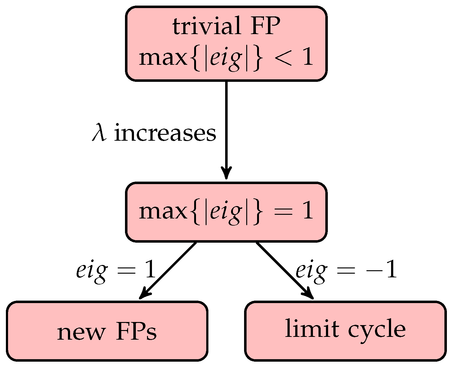
The immediate corollary of Theorem 2 and Lemma 1 is if there is a unique globally attracting fixed point, then its coordinates are equal. We will refer to fixed point with equal coordinates as trivial fixed point. The whole complex behaviour of positive neurons (and in such a way, fuzzy-rough cognitive networks) evolves from this trivial fixed point via bifurcations (see the flowchart Figure 3 for the way to the first bifurcation). In Section 5, we show that different size of FRCNs (different number of decision classes N) may show significantly different qualitative behaviour.

5. Dynamics of Positive Neurons

First we provide the Jacobian at the trivial fixed point. In general (except the case $N=2$), this fixed point is a function of $\lambda$ and N. Let us denote the coordinates of the trivial fixed point by $p^{\ast }$. Then the $(i,j)$ entry of the Jacobian of the mapping $f\left(W_{p}P\right)$ at this point, using the fact that $f\left(W_p{P}^{\ast }\right)=p^{\ast }$ and for the sigmoid function $f^{\prime }=\lambda f(1-f)$:

$$\frac{\partial f}{\partial p_i}{|}_{P=P^{\ast }}=\lambda f\left(W_p{P}^{\ast }\right)(1-f\left(W_p{P}^{\ast }\right))w_{ij}=\lambda p^{\ast }(1-p^{\ast })w_{ij}$$

(31)

The whoole Jacobian matrix evaluated at the trivial fixed point is the following:

$$J_{p^{\ast }}=\lambda p^{\ast }(1-p^{\ast })W_p.$$

(32)

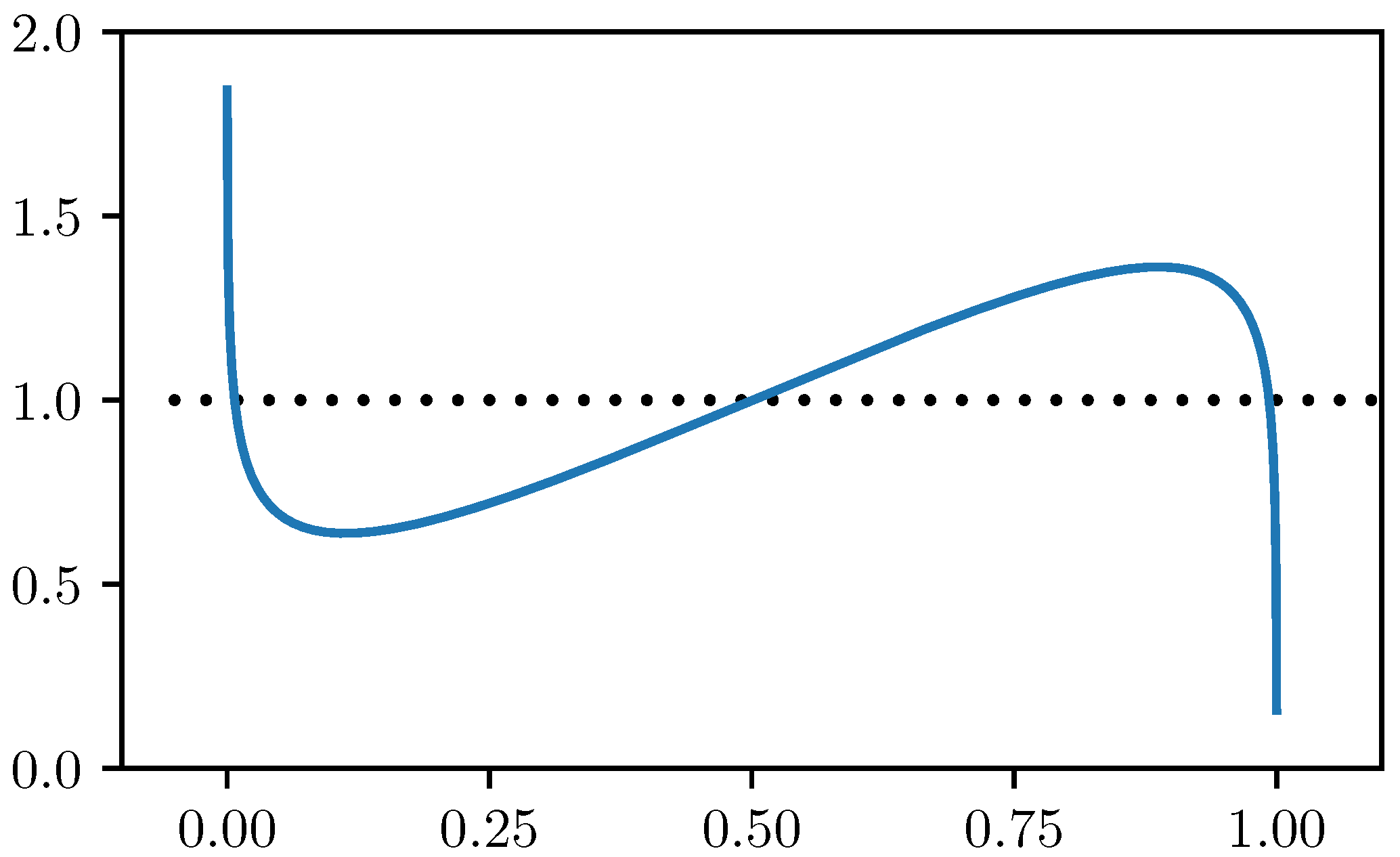
Its eigenvalues are $\lambda p^{\ast }(1-p^{\ast })$ times the eigenvalues of $W_p$: $(2-N)\lambda p^{\ast }(1-p^{\ast })$ and $2\lambda p^{\ast }(1-p^{\ast })$. As the value of $\lambda$ increases, at a certain point the absolute value of the eigenvalue with the highest modulus reaches one, the trivial fixed point loses its global stability and a bifurcation occurs. The type of this bifurcation has great effect on the further evolution and dynamics of the system. Based on the eigenvalues of $W_P$, we see that Neimark-Sacker bifurcation does not occur here, but saddle-node and perido-doubling bifurcations do play an important role.

5.1. $N=2$

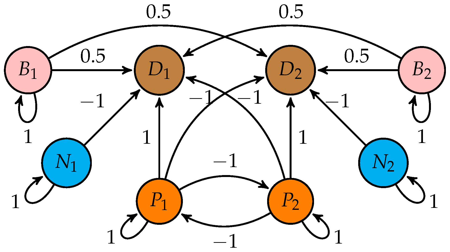
Consider first the case when we have only two decision classes. The relations between the positive neurons can be seen in Figure 1. The weight matrix describing the connections is the following (subscript P refers to positive):

$$W_P=\left[\begin{array}{cc}\hfill 1& \hfill -1\\ \hfill -1& \hfill 1\end{array}\right]$$

(33)

Easy to check the the point ${[0.5,0.5]}^T$ is always a fixed point of the mapping $f\left(W_{p}P\right)=P$, since

$$\left[\begin{array}{cc}\hfill 1& \hfill -1\\ \hfill -1& \hfill 1\end{array}\right]\left[\begin{array}{c}0.5\\ 0.5\end{array}\right]=\left[\begin{array}{c}0\\ 0\end{array}\right]$$

(34)

and $f\left(0\right)=0.5$. According to Theorem 2, if $\lambda <2$, then it is the only fixed point, moreover it is globally asymptotically stable, i.e., strating from any initial activation vector, the iteration will converge to this fixed point. The Jacobian of the mapping at this fixed point is

$$\lambda ·0.5(1-0.5)]\left[\begin{array}{cc}\hfill 1& \hfill -1\\ \hfill -1& \hfill 1\end{array}\right]=\frac{\lambda }{4}\left[\begin{array}{cc}\hfill 1& \hfill -1\\ \hfill -1& \hfill 1\end{array}\right]$$

(35)

and its eigenvalues are 0 and $\lambda /2$. When the eigenvalue $\lambda /2=1$ ($\lambda =2$), a bifurcation occurs, giving birth to two new fixed points. In the following, we are going to show that for every $\lambda >2$, there are exactly three fixed points, moreover these fixed points have the following coordinates: ${[0.5,0.5]}^T$, $[x^{\ast },1-x^{\ast }]$ and $[1-x^{\ast },x^{\ast }]$, where $x^{\ast }$ is a fixed point of a one dimensional mapping described below.

Let us assume that ${(x_1,x_2)}^T$ is a fixed point of the mapping, then

$$\left[\begin{array}{c}{x}_1\\ x_2\end{array}\right]=f\left(\left[\begin{array}{cc}\hfill 1& \hfill -1\\ \hfill -1& \hfill 1\end{array}\right]\left[\begin{array}{c}{x}_1\\ x_2\end{array}\right]\right)=\left(\begin{array}{c}f(x_1-x_2)\\ f(x_2-x_1)\end{array}\right)$$

(36)

Since f is the sigmoid function, we have that $f(-x)=1-f\left(x\right)$, consequently

$$\begin{array}{cc}\hfill x_1& =f(x_1-x_2),\hfill \end{array}$$

(37)

$$\begin{array}{cc}\hfill x_2& =f(x_2-x_1)=f(-(x_1-x_2))=1-f(x_1-x_2)=1-x_1.\hfill \end{array}$$

(38)

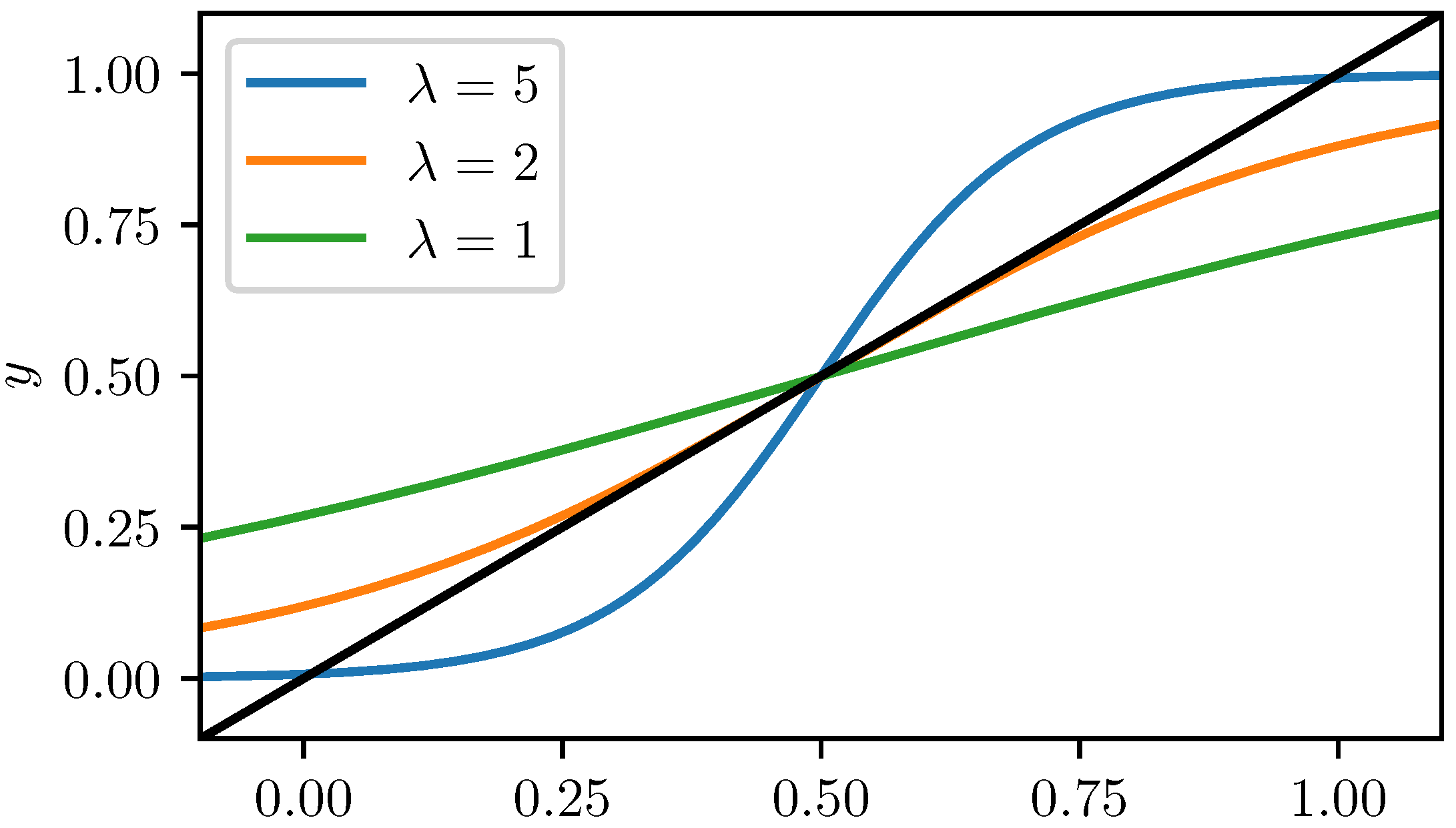
So for a fixed point the coordinates are $(x_1,1-x_1)$. The first equation leads to the following fixed point equation:

$$x_1=f(2x_1-1).$$

(39)

It means that the FPs of the positive neurons can be determined by solving Equation (39). From the graphical point of view, easy to see that if $\lambda \le 2$, then it has exactly one solution ($x_1=0.5$), but if $\lambda >2$, then there are three different solutions: $0.5$, $x^{\ast }$ and $1-x^{\ast }$ (see Figure 4).

From the analytical viewpoint, we have to solve the equation

$$x=\frac{1}{1+e^{-\lambda (2x-1)}}.$$

(40)

Applying the inverse of $f\left(x\right)$ and rearranginig the terms:

$$\frac{1}{\lambda }\ln \frac{1-x}{x}+2x=1$$

(41)

As it was pointed out in [37], if $\lambda >2$, then the left hand side has local minimum at $\frac{1}{2}-\sqrt{\frac{\lambda -2}{4\lambda }}$ less than one, and local maximum at $\frac{1}{2}+\sqrt{\frac{\lambda -2}{4\lambda }}$ greater than one. If $\lambda \le 2$, then the function is strictly monotone decreasing. Using continuity of the function, we conclude that there are exactly three solutions for every $\lambda >2$ and there is a unique solution if $\lambda \le 2$ (see Figure 5).

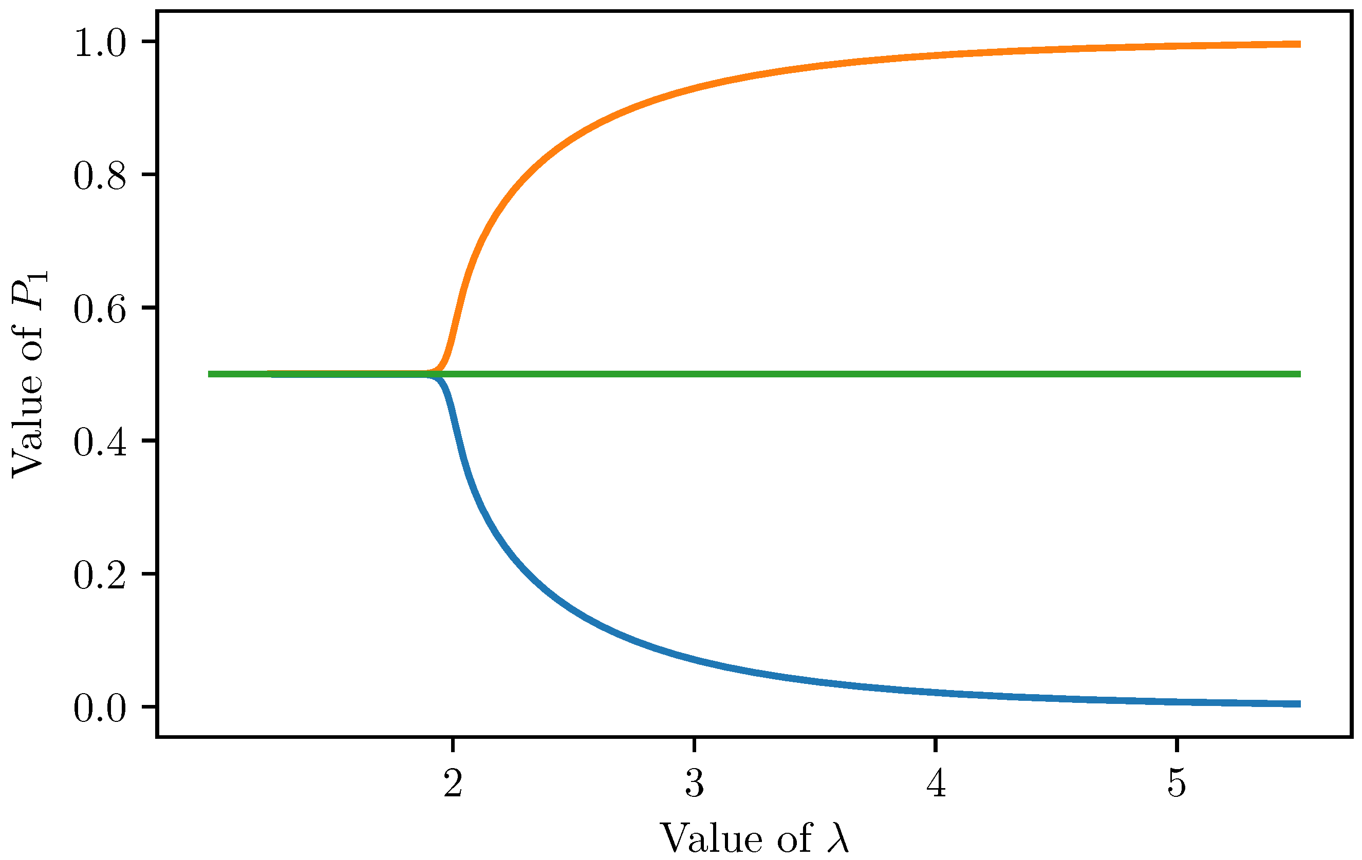
For $\lambda =5$, the fixed points are $(0.5,0.5)$, $(0.0072,0.9928)$ and $(0.9928,0.0072)$.

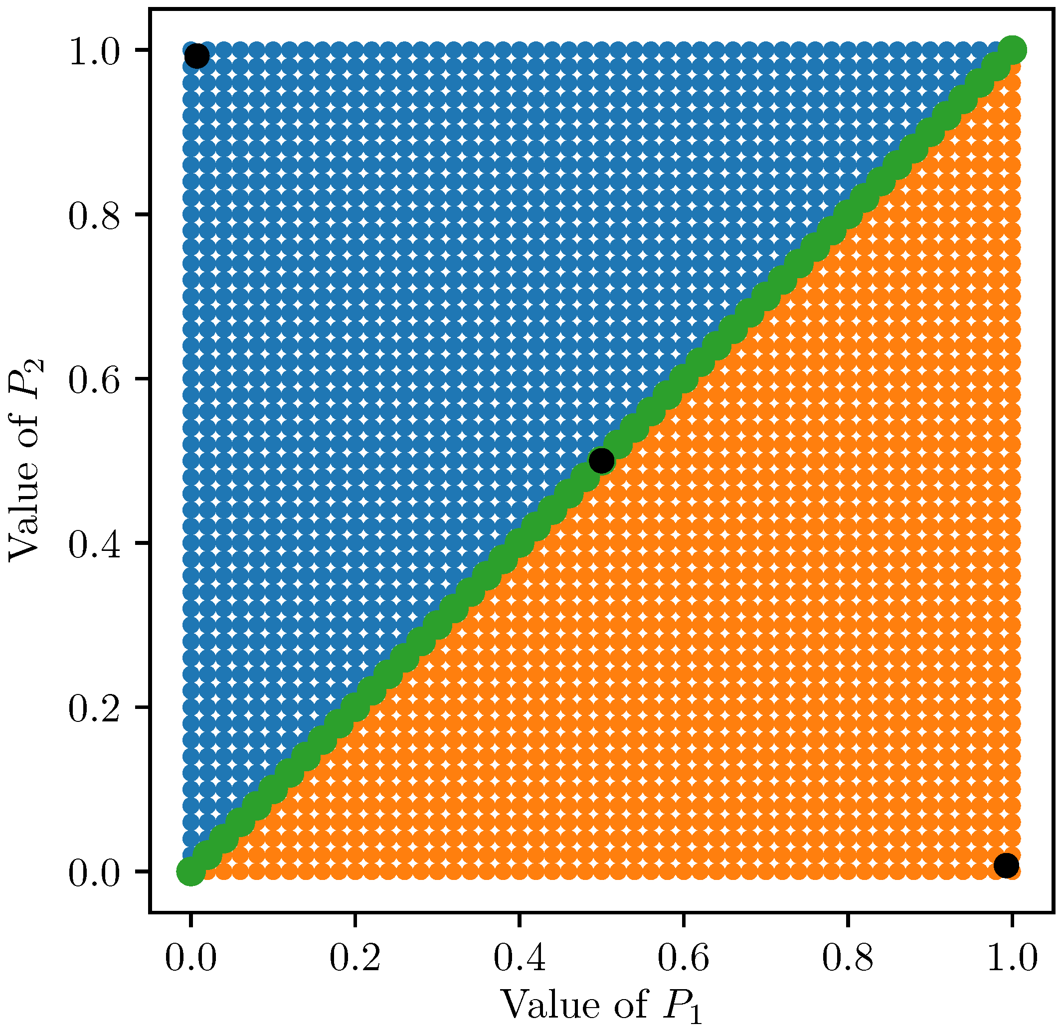
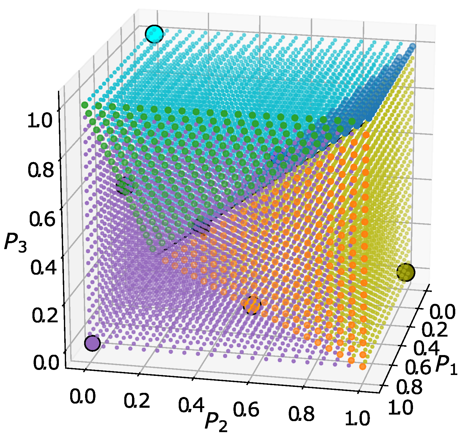
Let us examine the basins of attraction for the three different fixed points, i.e., $\lambda >2$ and the fixed points are ${[0.5,0.5]}^T$, $[x^{\ast },1-x^{\ast }]$ and $[1-x^{\ast },x^{\ast }]$, with $x^{\ast }>1/2$. Consider a point ${(x_1,x_2)}^T$ as initial activation vector (see Figure 6).

• If $x_1=x_2$, then the iteration leads to the fixed point $(0.5,0.5)$, since

  $$f\left(\left[\begin{array}{cc}\hfill 1& \hfill -1\\ \hfill -1& \hfill 1\end{array}\right]\left[\begin{array}{c}{x}_1\\ x_2\end{array}\right]\right)=\left[\begin{array}{c}f(x_1-x_2)\\ f(x_2-x_1)\end{array}\right]=\left[\begin{array}{c}f\left(0\right)\\ f\left(0\right)\end{array}\right]=\left[\begin{array}{c}0.5\\ 0.5\end{array}\right].$$

  (42)
• If $x_1>x_2$, then $f(x_1-x_2)>f\left(0\right)>f(x_2-x_1)$, so this ordering remains invariant during the iteration process. Moreover, after the first iteration step it reduces to a one dimensional iteration with initial value $x=f(x_1-x_2)>1/2$ and updating equation $x=f(2x-1)$. If $x>1/2$, then fixed point $x^{\ast }$ attracts this one-dimensional iteration. Consequently, the original two-dimensional itertaion converges to ${(x^{\ast },1-x^{\ast })}^T$.
• Similarly, if $x_1<x_2$, then the iteration ends in ${(1-x^{\ast },x^{\ast })}^T$.

The size of the basin of attraction can be considered as the number of its points. In the strict mathematical sense it is infinity, of course. On the other hand, the basin of fixed point $(0.5,0.5)$ is a one dimensional object (line segment), while the basins of $(x^{\ast },1-x^{\ast })$ and $(1-x^{\ast },x^{\ast })$ are two-dimensional sets (triangles), so they are ‘much more bigger’ sets.

In applications, we always work with sometimes large, but finite numbers of points, based on the required and available precision. Let us define the level of granularity as the length of subintervals, when we divide the unit interval into n equal parts. Then the division points are $0,1/n,2/n,\dots ,1$, so we have $n+1$ points. The basin of fixed point $(0.5,0.5)$ contains $n+1$ points, while the basins of the two other fixed points have $n(n+1)/2$, $n(n+1)/2$ points. By increasing the number of division points, the proportion of the basins tend to zero and $1/2$, as it was expected.

$$\begin{array}{cc}\hfill \underset{n\to \infty }{\lim }\frac{n+1}{{(n+1)}^2}& =0\hfill \end{array}$$

(43)

$$\begin{array}{cc}\hfill \underset{n\to \infty }{\lim }\frac{n(n+1)/2}{{(n+1)}^2}& =\frac{1}{2}\hfill \end{array}$$

(44)

In a certain sense, it means that fixed points ${(x^{\ast },1-x^{\ast })}^T$ and ${(1-x^{\ast },x^{\ast })}^T$ are more important than fixed point ${(0.5,0.5)}^T$, since much more initial activation values lead to these points.

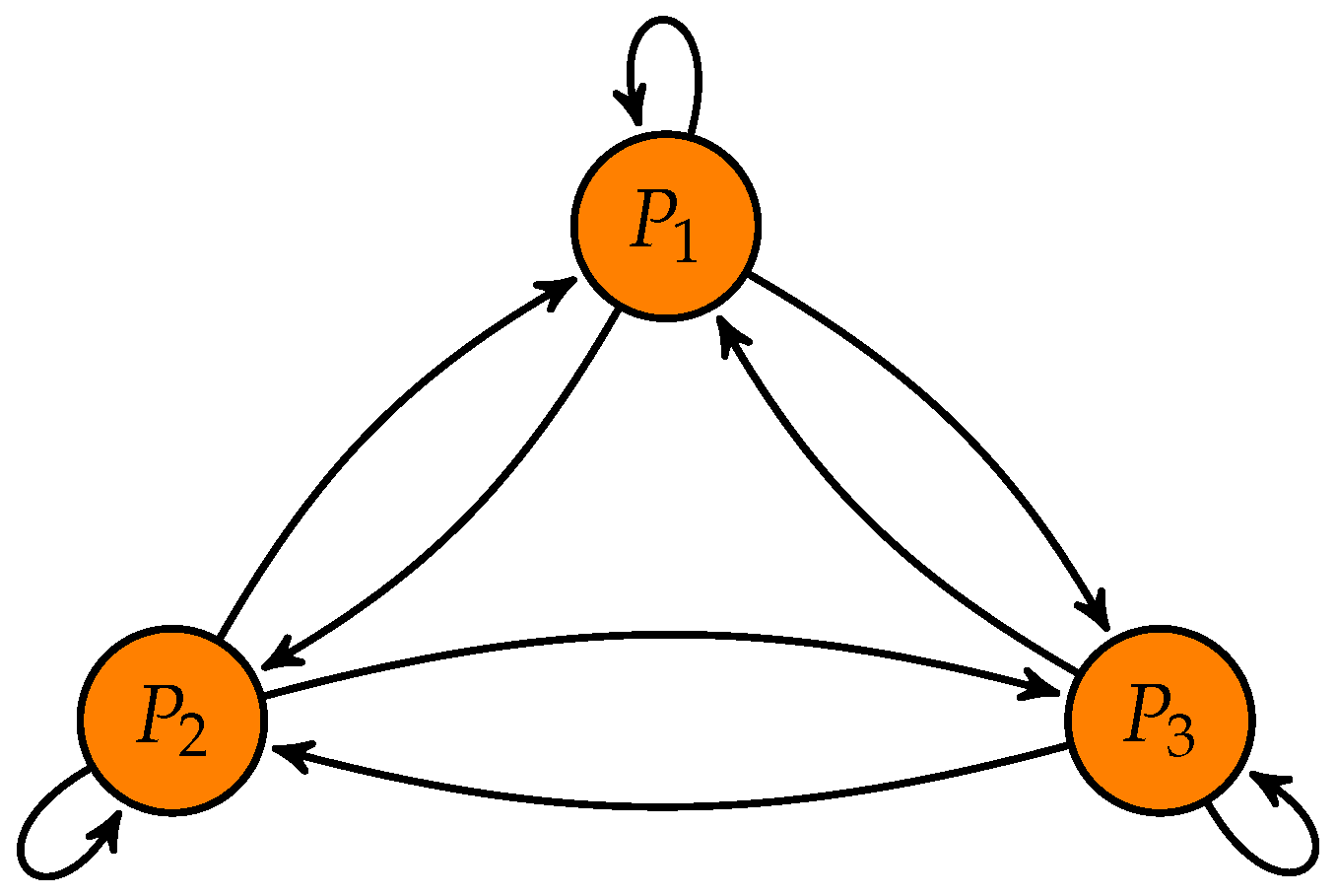
5.2. $N=3$

The structure of the connections between positive neurons can be seen in Figure 7. In this case, the eigenvalues of $W_P$ are $-1$ (with multiplicity one) and 2 (with multiplicity two). The fixed point with equal coordinates loses its global asymptotic stability when the absolute value of its larger eigenvalue equals one. Since the positive eigenvalue has the higher absolute value, this bifurcation results in new fixed points. Nevertheless, this eigenvalue has multiplicity two, so it is not a simple bifurcation, i.e., not only a pair of new fixed points arise, but a couple of new FPs. The trivial fixed point becomes a saddle point, i.e., it attracts points in a certain direction, but repells them in other directions. If we further increase the value of the parameter $\lambda$, then the absolute value of the negative eigenvalue reaches one and the trivial fixed point suffers a bifurcation again. Since the eigenvalue is $-1$, this is a period-doubling bifurcation, giving birth to a two-period limit cycle.

We show that there are three type of fixed points:

• The trivial fixed point with equal coordinates ($F{P}_0$);
• Fixed points with one high and two low values ($F{P}_1$);
• Fixed points with one low and two medium coordinates ($F{P}_2$).

The existence of $F{P}_0$ is clear, as it was shown by Lemma 1. As it was pointed out in Section 4, the non-trivial fixed points have two different coordinate values. Let us denote these values by x, x and y. Then the fixed point equation is

$$\left[\begin{array}{c}x\\ x\\ y\end{array}\right]=f\left(\left[\begin{array}{ccc}\hfill 1& \hfill -1& \hfill -1\\ \hfill -1& \hfill 1& \hfill -1\\ \hfill -1& \hfill -1& \hfill 1\end{array}\right]\left[\begin{array}{c}x\\ x\\ y\end{array}\right]\right)=\left(\begin{array}{c}f(-y)\\ f(-y)\\ f(y-2x)\end{array}\right),$$

(45)

which simplifies to the following system of equations:

$$\begin{array}{cc}\hfill x& =f(-y)\hfill \end{array}$$

(46)

$$\begin{array}{cc}\hfill y& =f(y-2x)\hfill \end{array}$$

(47)

By substituting x, we have

$$\begin{array}{cc}\hfill y& =f(y-2x)=f(y-2f(-y))=\frac{1}{1+e^{-\lambda (y-2f(-y\left)\right)}}=\frac{1}{1+e^{-\lambda \left(y-2\frac{1}{1+e^{\lambda y}}\right)}}\hfill \end{array}$$

(48)

It is again a fixed point equation, whose number of solutions depends on the value of parameter $\lambda$ (see Figure 8):

• if $\lambda \le 2.2857$ (rounded), then there is exactly one solution, it refers to the trivial fixed point ($F{P}_0$);
• if $\lambda >2.2857$, then there are three different solutions, one refers to $F{P}_0$, one to $F{P}_1$s and one to $F{P}_2$.

Using the values of y, we can determine the values of x. Furthermore, if y is high, then based on the equation $x=f(-y)=1-f\left(y\right)$, we may conclude that x is low. Similarly, if y is low, then x is medium. Finally, there are seven fixed points:

• the fixed point with equal coordinates ($F{P}_0$);
• three fixed points with one high and two low values ($F{P}_1$);
• three fixed points with one low and two medium values ($F{P}_2$s).

For $\lambda =5$, these fixed points are (rounded to four decimals)

• $(0.2355,0.2355,0.2355)$ ($F{P}_0$),
• $(0.9926,0.0069,0.0069)$ and its permutations ($F{P}_1$),
• $(0.4904,0.4904,0.0076)$ and its permutations ($F{P}_2$).

Initial activation values lead to these fixed points according to the following:

• if $P_1^0=P_2^{\left(0\right)}=P_3^{\left(0\right)}$, then the iteration converges to $F{P}_0$;
• if $P_1^0>P_2^{\left(0\right)}\ge P_3^{\left(0\right)}$, then the iteration converges to $F{P}_1$;
• if $P_1^0=P_2^{\left(0\right)}>P_3^{\left(0\right)}$, then the iteration converges to $F{P}_2$.

Ranking is preserved between positive neurons, in the sense that if $P_x^{\left(0\right)}\ge P_y^{\left(0\right)}$, then $P_x^{\ast }\ge P_y^{\ast }$. Since the number of possible outcomes is very limited (only three cases without permutations), it means that some differences in the initial activation values will magnified, for example if the initial activation vector is $(0.3,0.2,0.1)$, then the iteration converges to $(0.9926,0.0069,0.0069)$. On the other hand, some large differences will be hidden: initial activation vector $(1,0.95,0)$ leads again to $(0.9926,0.0069,0.0069)$.

Limit cycle occurs, when the negative eigenvalue of the Jacobian computed at the trivial fixed point reaches $-1$ (at about $\lambda =5.8695$). Similarly to the trivial fixed point, the elements of the limity cycle have equal coordinates. Let us denote these points by $(x_1,x_1,x_1)$ and $(x_2,x_2,x_2)$. The members of a two-period limit cycle are fixed points of the double iterated function.

$$\left[\begin{array}{c}{x}_1\\ x_1\\ x_1\end{array}\right]=f\left(W_P\left[\begin{array}{c}{x}_2\\ x_2\\ x_2\end{array}\right]\right)\mathrm{and}\left[\begin{array}{c}{x}_2\\ x_2\\ x_2\end{array}\right]=f\left(W_P\left[\begin{array}{c}{x}_1\\ x_1\\ x_1\end{array}\right]\right)$$

(49)

In coordinate-wise form this provides the following system of equations:

$$\begin{array}{cc}\hfill x_1& =f(-x_2)\hfill \end{array}$$

(50)

$$\begin{array}{cc}\hfill x_2& =f(-x_1)\hfill \end{array}$$

(51)

From which we have

$$x_2=f(-x_1)=f(-f(-x_2))=\frac{1}{1+e^{\lambda f(-x_2)}}=\frac{1}{1+e^{\lambda \frac{1}{1+e^{\lambda x_2}}}}$$

(52)

If $\lambda \le 5.8695$, then it has a unique solution. It refers to the trivial fixed point, since this point is a fixed point of the double-iterated function, too. If $\lambda >5.8695$, then there are two other solutions, low and medium, these are the coordinates of the two-period limit cycle. For example, for $\lambda =7$, these points are $0.0563$ and $0.4027$.

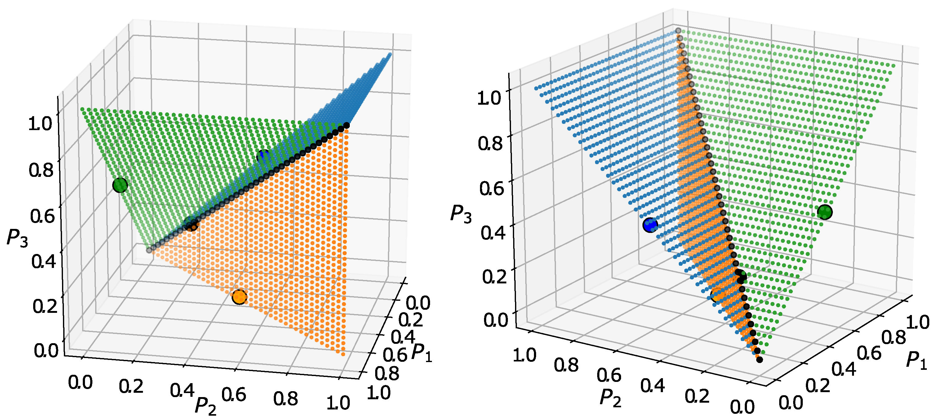
For a general case, basins of attraction of a dynamical systems are difficult to determine and sometimes it is analytically not feasible task [41,42], enough to mention the famous graph of Newton’s method’s basin ofattractions [43]. We examined the basin of attraction of the fixed points by putting an equally spaced grid on the set of possible initial values of positive neurons $P_1$, $P_2$ and $P_3$, and applied the grid points as initial activation values.

Table 1. Number of points in basin of attraction in percentage of the total number of points for $N=3$ decision classes, $\lambda =5$. $F{P}_0$ refers to fixed point with equal coordinates, $F{P}_1$ refers to fixed points with one high and two low values, while $F_2$ refers to fixed points with two medium and one low values.

Number of Classes	Granurality	FP0	FP1	FP2	LC	Total Number of Points
$N=3$	0.5	11.11	55.56	33.33	0	$3^3$
	0.25	4.00	72.00	24.00	0	$5^3$
	0.2	2.78	76.39	20.83	0	$6^3$
	0.1	0.83	86.78	12.39	0	${11}^3$
	0.05	0.23	92.97	6.80	0	${21}^3$
	0.01	0.01	98.52	1.47	0	${101}^3$

shows the sizes of the basins of attraction for different granurality. Results are visualized in Figure 9 and Figure 10.

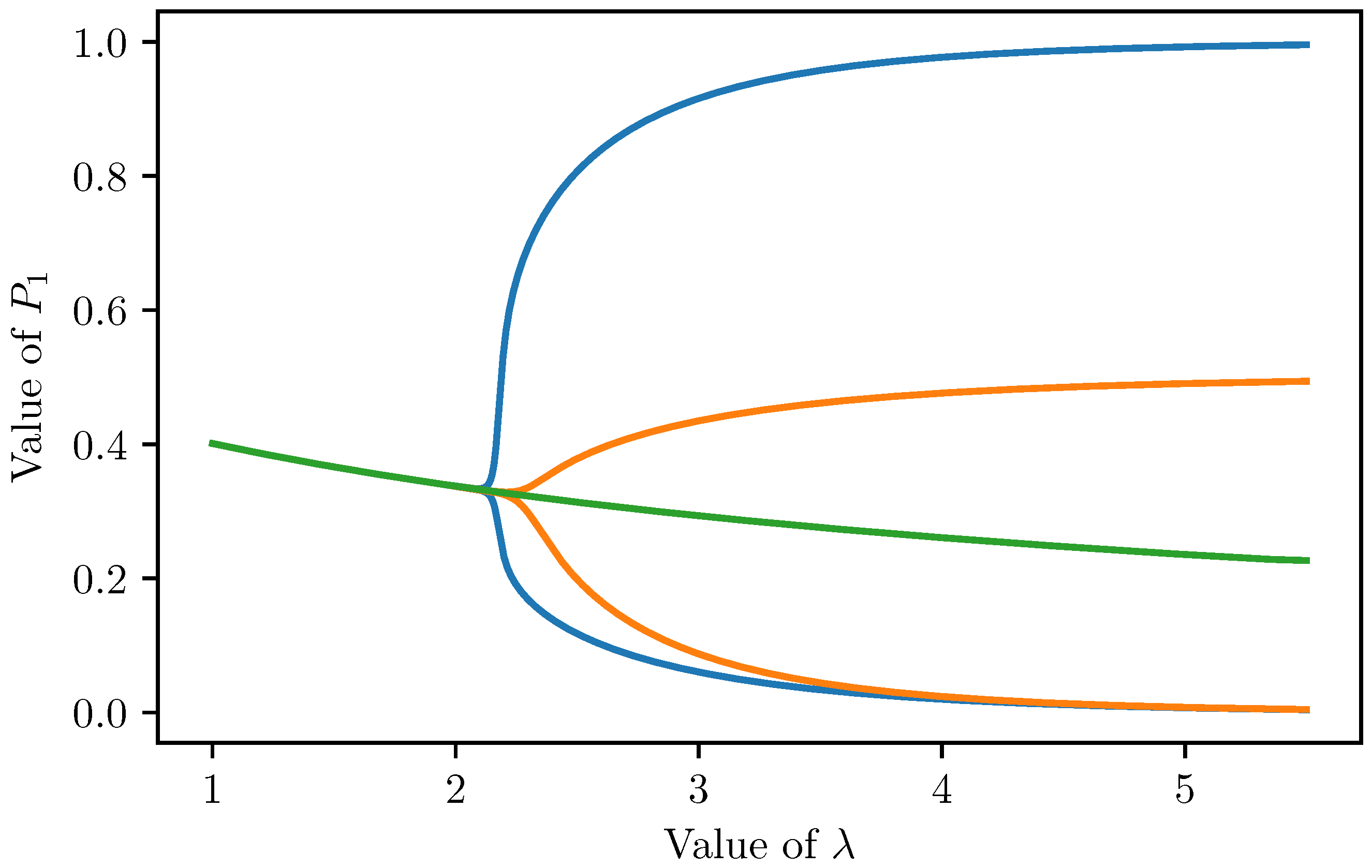
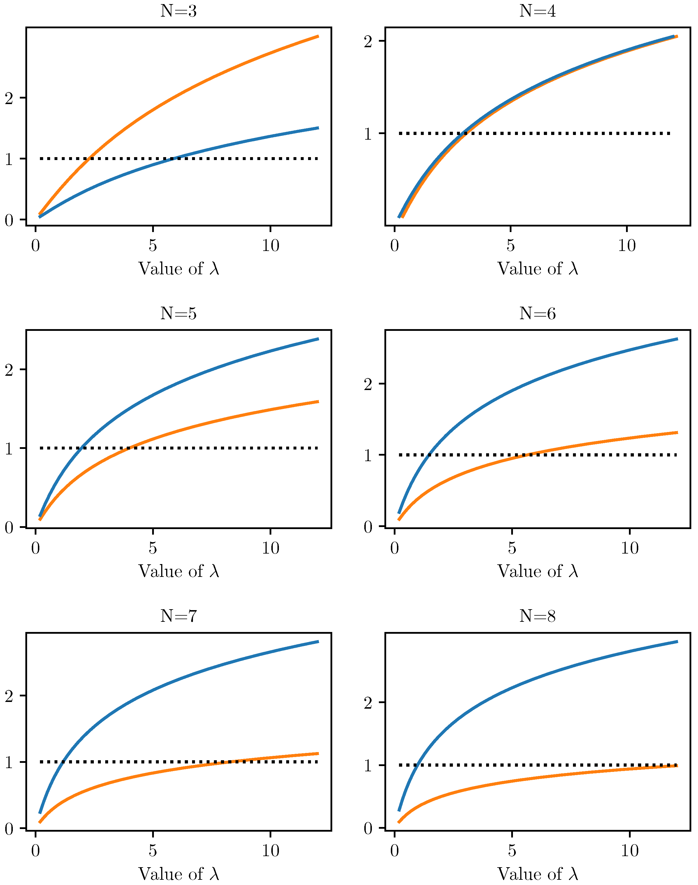
5.3. $N\ge 4$

If the FRCN has $N=4$ decision classes, then the eigenvalues of the Jacobian at the trivial fixed point have the same magnitude, but with different sign. So positive and negative eigenvalues reaches one (in absolute value) at the same value of parameter $\lambda$ (see Figure 11), causing the appearance of new fixed points and limit cycle simultaneuosly. The trivial fixed point is no longer an attractor, but fixed points with pattern one high, three low and two medium, two low values do exists.

If $N\ge 5$, then the absolute value of the negative eigenvalue of the Jacobian evaluated at the trivial fixed point is higher then the positive value, consequently first a period-doubling bifurcation occurs and the trivial fixed point loses its attractiveness. We should note that occurence of fixed points of type $F{P}_1$ and $F{P}_2$ is not linked to the other (positive) eigenvalue, since they occur earlier, for a smaller value of $\lambda$.

For the general case (N decision classes), there exist two types of fixed points with the following patterns: one high, $N-1$ low values and two medium, $N-2$ low values. The fixed point equations for the one high ($x_1$), $N-1$ low ($x_2$) pattern

$$\begin{array}{cc}\hfill x_1& =f(x_1-(N-1)x_2)\hfill \end{array}$$

(53)

$$\begin{array}{cc}\hfill x_2& =f(-x_1-(N-3)x_2),\hfill \end{array}$$

(54)

which leads to the following one-dimensional fixed point problem:

$$x_1=(N-1)f\left(\frac{4-2N}{N-1}+\frac{N-3}{N-1}{f}^{-1}\left(x_1\right)\right)+f^{-1}\left(x_1\right)$$

(55)

The pattern two medium ($x_1$), $N-2$ low ($x_2$) values leads to the following equations:

$$\begin{array}{cc}\hfill x_1& =f(-(N-2)x_2)\hfill \end{array}$$

(56)

$$\begin{array}{cc}\hfill x_2& =f(-2x_1-(N-4)x_2),\hfill \end{array}$$

(57)

from which we get the a one-dimensional fixed point problem:

$$x_2=-\frac{1}{N-4}{f}^{-1}\left(x_2\right)-\frac{2}{N-4}f\left(-(N-2)x_2\right)$$

(58)

Nevertheless, these fixed points are less important for multiple decision classes.

Finally, we provide a geometrical reasoning of the structure of fixed points. Consider two fixed points of type $F{P}_1$, i.e., they have one high and $N-1$ low coordinates. Their basins of attractions are separated by a set, whose points do belong to none of them, but lie on an $N-1$ dimensional hyperplane ‘between’ them. Without loss of generality, we may assume that one fixed point is $P_1^{\ast }=(\alpha ,\beta ,\dots ,\beta )$ and the other one is $P_2^{\ast }=(\beta ,\alpha ,\beta ,\dots ,\beta )$. Because of symmetry, the hyperplane is perpendicular the line connecting $P_1^{\ast }$ and $P_2^{\ast }$, i.e., its normal vector is paralel to $\overrightarrow{P_1^{\ast }{P}_2^{\ast }}=(\beta -\alpha ,\alpha -\beta ,0,\dots ,0)$. Additionally, the hyperplane crosses the line at the middle point of $P_1^{\ast }$ and $P_2^{\ast }$, which has coordinates $\left(\frac{\alpha +\beta }{2},\frac{\alpha +\beta }{2},\beta ,\dots ,\beta \right)$. Consequently, the equation of the separating hyperplane is $x_1=x_2$. The separating set is a subset of this plane with the additional constrain $x_i<x_1$, for every $i\ne 1,2$. Consequently, a fixed point of type $F{P}_2$ has two medium coordinates with equal values ($x_1=x_2$), and $N-2$ equal, but low coordinates. Since there are N fixed points of type $F{P}_1$, there are $\left(\begin{array}{c}N\\ 2\end{array}\right)$ fixed points of type $F{P}_2$.

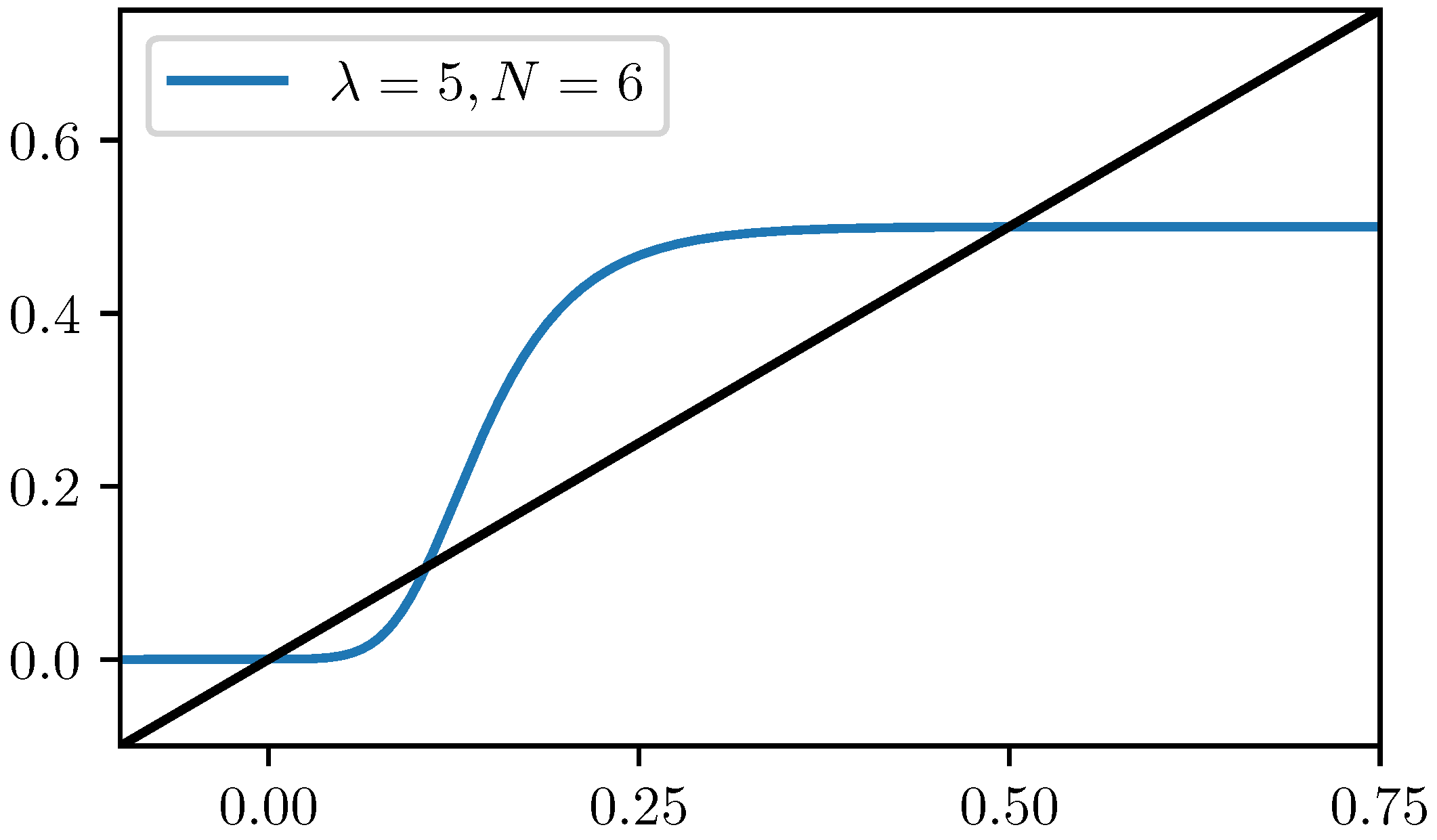
Simulation results show, that for $N\ge 4$, limit cycles tend to steal the show. Limit cycle oscillates between two activation vectors with equal coordinates (the equality of the coordinates is an immediate consequence of symmetry). Let us denote these points by $(x_1,\dots ,x_1)$ and $(x_2,\dots ,x_2)$. The members of a two-period limit cycle are fixed points of the double iterated function.

$$\left[\begin{array}{c}{x}_1\\ ⋮\\ x_1\end{array}\right]=f\left(W_P\left[\begin{array}{c}{x}_2\\ ⋮\\ x_2\end{array}\right]\right)\mathrm{and}\left[\begin{array}{c}{x}_2\\ ⋮\\ x_2\end{array}\right]=f\left(W_P\left[\begin{array}{c}{x}_1\\ ⋮\\ x_1\end{array}\right]\right)$$

(59)

In coordinate-wise form this gives the following system of equations:

$$\begin{array}{cc}\hfill x_1& =f(-(N-2)x_2)\hfill \end{array}$$

(60)

$$\begin{array}{cc}\hfill x_2& =f(-(N-2)x_1)\hfill \end{array}$$

(61)

From which we have

$$x_2=f(-(N-2)x_1)=f(-(N-2)f(-(N-2)x_2))=\frac{1}{1+e^{\lambda (N-2)\frac{1}{1+e^{\lambda (N-2)x_2}}}}.$$

(62)

For $\lambda$ values generally applied in fuzzy cognitive maps and for $\lambda =5$ used in FRCNs, this fixed point equation has three solutions: one refers to the trivial fixed point, which is no longer a fixed point attractor, the other two (low and medium) are coordinates of the elements of the limit cycle (see Figure 12).

Simulation results show that by increasing the number of decision classes, more and more initial values arrive to a limit cycle. We put equally spaced N dimensional grid on the set ${[0,1]}^N$ with stepsize $0.5$, $0.25$, $0.2$ and $0.1$, then applied the gridpoints as initial activation values of the positive neurons. Since any particular real-life dataset finally turns into initial activation values for the FRCN model, it means that these gridpoints can be viewed as representations of possible datasets, up to the predefined precision (i.e., step size). Iteration stopped when convergence or limit cycle was detected or the predefined maximum numbers of steps reached. As we can observe in

Table 2. Number of points in basin of attraction in percentage of the total number of points, for different number of classes (N) and level of granularity, $\lambda =5$. $F{P}_1$ refers to fixed points with one high and $N-1$ low values, while $F_2$ refers to fixed points with two medium and $N-2$ low values, $LC$ stands for limit cycle.

Number of Classes	Granurality	FP0	FP1	FP2	LC	Total Number of Points
$N=4$	0.5	0	39.51	14.81	45.68	$3^4$
	0.25	0	48.64	9.60	41.76	$5^4$
	0.2	0	45.68	6.02	48.30	$6^4$
	0.1	0	48.77	3.36	47.87	${11}^4$
	0.05	0	50.34	1.41	48.25	${21}^4$
$N=5$	0.5	0	24.69	8.23	67.08	$3^5$
	0.25	0	27.52	0.96	71.52	$5^5$
	0.2	0	23.21	2.06	74.73	$6^5$
	0.1	0	17.34	0.50	82.16	${11}^5$
	0.05	0	16.24	0.14	83.62	${21}^5$
$N=6$	0.5	0	13.99	4.12	81.89	$3^6$
	0.25	0	7.22	0.29	92.49	$5^6$
	0.2	0	7.52	0.13	92.35	$6^6$
	0.1	0	4.75	0.04	95.21	${11}^6$
$N=7$	0.5	0	7.36	1.92	90.72	$3^7$
	0.25	0	2.72	0.08	97.20	$5^7$
	0.2	0	1.90	0.03	98.07	$6^7$
	0.1	0	1.13	0.00	98.87	${11}^7$
$N=8$	0.5	0	3.66	0.00	96.34	$3^8$
	0.25	0	0.95	0.00	99.05	$5^8$
	0.2	0	0.60	0.00	99.40	$6^8$
	0.1	0	0.03	0.00	99.97	${11}^8$

, most of the initial values finally arrive to a limit cycle.

6. Relation to Decision

It has been proved previously, that values of negative and boundary neurons converge to the same value (it is ≈ 0.9930 for $\lambda =5$) and the dynamical behaviour of positive neurons was analyzed in the preceding sections. Now we examine their effect on the decision neurons and such a way, on the final decision.

Decision neurons have only input values, they do not influence each other, neither other types of neurons. As a consequence, the sigmoid transfer function $f\left(x\right)$ only transform their values into the $(0,1)$ interval, but does not change the order of the values (with respect to the ordering relation ‘≤’), since $f\left(x\right)$ is strictly monotone increasing. Before analyzing the effects of the results of the previous sections, we briefly summarize the conclusion of [37]: assuming that the activation values of positive neurons reach a stable state, they concluded that negative neurons have no influence on FRCNs’ performance, but the ranking of positive neurons’ activation values and the number of boundary neurons connected to each decision neuron have high impact. Based on the previous sections, below we ad some more insights to this result.

If positive neurons reach a stable state (fixed point), then this stable state have either the pattern one high and $N-1$ low values ($F{P}_1$) or two medium and $N-2$ low values ($F{P}_2$), the trivial fixed point with equal coordinates ($F{P}_0$) plays a rule only for 2 and 3 decision classes. These values are unique and completely determined by the parameter $\lambda$ and the number of decision classes N. It means that the number of possible final states is very limited. This fact was mentioned in the case of $N=3$ decision classes, but valid for every $N\ge 3$ cases. Namely, small differences between the initial activation vales could be magnified by the exploitation phase. Almost equal initial activation values with proper maximum lead to the pattern of one high and $N-1$ low values, resulting in something like a winner-takes-all rule. Although the runner-up has only a little smaller initial value, after reaching the stable state, it needs the same number of boundary connections to overcome the winner, as the one with very low initial value needs.

If the maximal number of iterations is reached without convergence (i.e., the activation value vector oscillates in a limit cycle), then the iteration is stopped and the last activation vector is taken. It has either $(low,\dots ,low)$ or $(medium,\dots ,medium)$ pattern with equal coordinates. In this case, the positive neurons have absolutely no effect on the final decision. The classification goes to the neuron with the highest number of boundary connections, regardless of the small or large differences between the initial activation values of the positive neurons.

7. Conclusions and Future Work

The behaviour of fuzzy-rough cognitive networks was studied applying the theory of discrete dynamical systems and their bifurcations. The dynamics of negative and positive neurons was fully discussed in lthe iterature, so we focused on the behaviour of positive neurons. It was pointed out, that the number of fixed points is very limited and their coordinate values follow a specific pattern ($F{P}_0$, $F{P}_1$, $F{P}_2$). Additionally, it was proved that when the number of decision classes is greater than three, the limit cycles unavoidably occur, causing the recurrent reasoning inconclusive. Simulations show that proportion of initial activation values leading to limit cycles increases with the number of decision classes, and the waste number of scenarios lead to oscillation. In this case, the decision relies totally on the number of boundary neuron connected to each decision neurons, regardless of the initial activation value of positive neurons.

The method applied in the paper may be followed in the analysis of other FCM-like models. As we have seen, if the parameter of the sigmoid threshold function is small enough, then an FCM has one and only one fixed point, which is globally asymptotically stable. If we increase the value of the parameter, then a fixed-point bifurcation occurs, causing an entirely different dynamical behaviour. If the weight matrix has a nice structure, for example in the case of positive neurons, then there is a chance to find the unique fixed point in a simple form or as a limit of a lower-dimensional iteration and determine the parameter value at the bifurcation point. Similarly, based on the eigenvalues of the Jacobian evaluated at this fixed point we can determine the type of bifurcation. Nevertheless, general FCMs have no well-structured weight matrices, since weights are usually determined by human experts or learning methods. It means some limitations on the generalization of the method applied. Theoretically, we can find unique fixed points and the bifurcation point, but this task is much more difficult for a general weight matrix.

Another exciting and important research direction is the possible generalization of the results to the extensions of fuzzy cognitive maps. Some well-known extensions are fuzzy grey cognitive maps (FGCMs) [44], interval-valued fuzzy cognitive maps (IVFCMs) [45], intuitionistic fuzzy cognitive maps (IFCMs) [46,47], temporal IFCMs [48], the combination of fuzzy grey and intuitionistic FCMs [49], interval-valued intuitionistic fuzzy cognitive maps (IVIFCMs) [50]. This future work probable requires deep mathematical inspection on interval-valued dynamical systems and may lead to several new theoretical and practical results on interval-valued cognitive networks, as well.