Effective Boundary Value Problem Solver via Bézier Functions

Abstract

In engineering disciplines, many important problems are to be formed as boundary value problems (BVPs) that have conditions that are specified at the extremes. To handle such problems, the conventional shooting method that transforms BVPs into initial value problems has been extensively used, but it does not always guarantee solving the problem due to the possible failure of finding a proper initial guess. This paper proposes a universal initial guess finder that is composed of Bézier functions. Various dimensional problems that include Lambert’s problem for several orbits around the spherically symmetric Earth are studied to validate the efficacy of the proposed approach, and the results are compared.

1. Introduction

Boundary value problems (BVPs) are important problems in engineering fields because plenty of problems are formed as BVPs that are given by the differential equations with boundary conditions (BCs). In celestial mechanics, for example, Lambert’s problem is the classical problem that is to determine an orbit by solving BVPs [1,2]. The goal of this problem is to find an orbit between two prescribed positions within a given fixed time of flight. The orbit determination, which solves Lambert’s problem, is usually utilized for spacecraft intercept [3], rendezvous [4], orbit transfer [5], etc. A general solving approach for BVPs is the shooting method that finds unknown initial values that satisfy the given BCs. For orbit determination, it requires finding the initial velocity that corresponds to the prescribed position at the initial time. For applying the shooting method, the main challenge is to determine a suitable initial guess, because it may fail to find the solution depending on the starting guess selected. Developing an effective approach for selecting a proper initial guess is essential, because the initial guess affects not only the convergence rate of the solution, but also the success of obtaining the solution. Hence, this research proposes a novel approach to provide an appropriate initial guess for solving BVPs.

Bézier functions (BFs) are parametric functions that can describe complicated surfaces and curves with great flexibility [6,7,8]. These parametric functions are composed of linear combinations of polynomials and the coefficients that are called the control points, which can adjust the shape of curves. BFs have been investigated for describing trajectories in a variety of studies: airfoil design [9], path planning [10,11,12,13,14,15], collision avoidance [16,17,18,19], trajectory generation [20], etc. Besides, studies that are associated with the celestial mechanics by utilizing BFs are conducted by several researchers. Dilectis and Mortari [21] used BFs to describe orbit trajectories by only utilizing observations. Pan and Ma designed a formulation of Lambert’s problem with respect to the argument of periapsis by using BFs [22]. Mortari and Clocchiatti [23] utilized non-rational BFs (NBFs) by approximating Kepler’s equation for the entire mean anomaly range, and a root-finding tool by using BFs for solving Kepler’s equation was proposed by Mortari and Elipe [24]. In addition, Kim and Mortari [25] found closed-form solutions for conic section descriptions using rational BFs (RBFs) and proposed an idea to solve two-point BVPs via NBFs.

This work utilizes BFs to provide a suitable initial guess to efficiently and successfully solve BVPs. Being inspired by the characteristics of coefficients (control points) of BFs and the research studied by Kim and Mortari [25], a solution trajectory of the given BVPs is approximated by adjusting BFs’ coefficients that are control points and weights. From the approximated trajectory, the initial guess is easily computed at the lower bound. Becuase this initial guess is close to the initial value to be obtained, the unknown initial value can be effectively found by applying the initial guess obtained by BFs into the shooting method. In order to validate the proposed approach, numerical simulation studies are performed for several BVPs, including an orbit determination problem. Before applying the proposed approach into the orbit determination problems, it considers one-dimensional (1D) and 2D BVPs as examples. Subsequently, the proposed approach is applied to the orbit determination problem for multiple orbits around the Earth that is spherically symmetric with various initial positions.

2. Method

BFs can approximate arbitrary curves by adjusting the control points and the relative weights. It is important to note that the weights are only applicable for RBFs that are explained in Section 2.1. Inspired by the characteristics of the endpoints among the control points, an effective initial guess finding approach for solving BVPs is proposed.

2.1. Bézier Functions

BFs are implicit functions that can describe complicated curves and surfaces [6,25], and there are two types: NBFs and RBFs. The shape of curves is mainly ruled by the control points, but RBFs have additional factors that can control the shape of curves, which are weights that are associated with the control points. Both types of BFs are composed of Bernstein polynomials (BPs) and a set of control points (and additional weights for RBFs). BPs of degree n is defined as [26,27]

$$b_{n,k}\left(s\right)=\left(\genfrac{}{}{0pt}{}{n}{k}\right)s^k{(1-s)}^{n-k},$$

(1)

where $\left(\genfrac{}{}{0pt}{}{n}{k}\right)$ is a binomial coefficient, $k=0,1,\cdots ,n$, and $s\in [0,1]$ is the implicit parameter. BPs have several properties as follows: [26,27,28]

• BPs $b_{n,k}\left(s\right)$ and $b_{n,n-k}\left(s\right)$ are mirror images of each other about the interval mid-point $s=1/2$ (i.e., $b_{n,n-k}(1-s)=b_{n,k}\left(s\right)$);
• there is the recurrent relation between BPs of degree $n+1$ and n as $b_{n+1,k}\left(s\right)=(1-s)b_{n,k}+s{b}_{n,k-1}$;
• they are non-negative as $b_{n,k}\left(s\right)\ge 0$ for $s\in [0,1]$;
• they form a partition of unity, ${\displaystyle \sum _{k=0}^n{b}_{n,k}\left(s\right)=1}$$\forall s$;
• the derivative of BP is defined as ${\displaystyle \frac{\mathrm{d}}{\mathrm{d}s}}{b}_{n,k}\left(s\right)=n[b_{n-1,k-1}\left(s\right)-b_{n-1,k}\left(s\right)]$;
• they are linearly independent, that is, $a_0{b}_{n,0}\left(s\right)+a_1{b}_{n,1}\left(s\right)+\cdots +a_n{b}_{n,n}\left(s\right)=0$;
• they can always be written as a linear combination of polynomials of higher degree, $b_{n-1,k}\left(s\right)={\displaystyle \frac{n-k}{n}}{b}_{n,k}\left(s\right)+{\displaystyle \frac{k+1}{n}}{b}_{n,k+1}\left(s\right)$; and,
• they span the full space of polynomials. This means that any n-degree polynomial can be expressed as a linear combination of n-degree BPs.

Note that BPs are the parametric basis function of both NBFs and RBFs.

A NBF of degree n is defined as [8,28]

$$p\left(s\right)=\sum _{k=0}^n{b}_{n,k}\left(s\right)c_k,$$

(2)

where $c_k$ is the k-th control point. A set of control points ($n+1$ number of points) is defined from $c_0$ through $c_n$. The first and last control points ($c_0$ and $c_n$) are called endpoints that indicate the start and end points of the curve. While the endpoints are located on the curve, the intermediate control points ($c_1,\cdots ,c_{n-1}$) do not lie on the curve [29]. Instead, the intermediate control points mainly control the shape of the curve. Because the endpoints lie on each end of the curve, one or more intermediate control points are required to generate a curve. That is, at least a quadratic BF is needed to approximate a curve. The r-th derivative of the NBF of degree n with respect to s is recursively defined as [28]

$$p^{\left(r\right)}\left(s\right)=\sum _{k=0}^{n-r}{b}_{n-r,k}\left(s\right)c_k^{\left(r\right)},$$

(3)

where

$$c_k^{\left(r\right)}=n(n-1)\cdots (n-r+1)\sum _{l=0}^r{(-1)}^{r-l}\left(\genfrac{}{}{0pt}{}{r}{l}\right)c_{k+l}.$$

(4)

An RBF of degree n is defined as [8,28]

$$p\left(s\right)=\frac{{\displaystyle \sum _{k=0}^n{w}_k{b}_{n,k}\left(s\right)c_k}}{{\displaystyle \sum _{k=0}^n{w}_k{b}_{n,k}\left(s\right)}},$$

(5)

where $w_k$ is the relative weight that is associated with k-th control point. By adding the weights, the RBFs have more flexibility than the NBFs because the RBFs have more parameters to be adjusted. That is, the RBFs can closely approximate arbitrary curves by adjusting both the weights and the control points. In order to determine the derivative of the RBF, the numerator and denominator are redefined as $p_n\left(s\right)$ and $p_d\left(s\right)$, and then Equation (5) is rewritten as $p\left(s\right)=p_n\left(s\right)/p_d\left(s\right)$. Subsequently, the r-th derivative of the RBF of degree n with respect to s is recursively derived as [28]

$$p^{\left(r\right)}\left(s\right)=\frac{{\displaystyle p_n^{\left(r\right)}\left(s\right)-\sum _{l=1}^r\left(\genfrac{}{}{0pt}{}{r}{l}\right)p_d^{\left(l\right)}\left(s\right)p^{r-l}\left(s\right)}}{p_d\left(s\right)},$$

(6)

where the derivatives of $p_n\left(s\right)$ and $p_d\left(s\right)$ are obtained by using Equations (3) and (4).

2.2. Shooting Method

A general form of nonlinear BVPs is given by

$$\mathit{g}(t,\mathbf{x}\left(t\right),\dot{\mathbf{x}}\left(t\right),\ddot{\mathbf{x}}\left(t\right))=\ddot{\mathbf{x}}\left(t\right)-\mathit{f}(t,\mathbf{x}\left(t\right),\dot{\mathbf{x}}\left(t\right))=\mathbf{0},$$

(7)

that satisfies the BCs $\mathbf{x}\left(t_{\mathrm{i}}\right)={\mathbf{x}}_{\mathrm{i}}$ and $\mathbf{x}\left(t_{\mathrm{f}}\right)={\mathbf{x}}_{\mathrm{f}}$. Here, $t\in [t_{\mathrm{i}},t_{\mathrm{f}}]$ is the time span that is set with the initial and final time $t_{\mathrm{i}}$ and $t_{\mathrm{f}}$, $\mathbf{x}\left(t\right)\in {\mathbb{R}}^m$ is the state vector, $\mathit{g}\in {\mathbb{R}}^m$ and $\mathit{f}\in {\mathbb{R}}^m$ are the nonlinear functions, and the subscripts i and f indicate the initial and final parameters, which also represent the lower and upper bounds. Note that $\mathit{g}$ is to be called the residual. The BVP is generally solved by using the shooting method that finds the solution of the given problem by using the solutions to a sequence of initial value problems (IVPs), and this problem is for solving Equation (7) with $\mathbf{x}\left(t_{\mathrm{i}}\right)={\mathbf{x}}_{\mathrm{i}}$ and $\dot{\mathbf{x}}\left(t_{\mathrm{i}}\right)={\mathbf{z}}_k$. Here, the unknown initial state ${\mathbf{z}}_k$ is initially set to be ${\mathbf{z}}_0$. Afterwards, ${\mathbf{z}}_k$ is selected in a manner to ensure that [30]

$$\underset{k\to \infty }{lim}\mathbf{x}(t_{\mathrm{f}},{\mathbf{z}}_k)=\mathbf{x}\left(t_{\mathrm{f}}\right)={\mathbf{x}}_{\mathrm{f}},$$

(8)

where $\mathbf{x}(t_{\mathrm{f}},{\mathbf{z}}_k)$ denotes the state at $t_{\mathrm{f}}$ when ${\mathbf{z}}_k$ is applied to the IVP in Equation (7), and $\dot{\mathbf{x}}\left(t_{\mathrm{i}}\right)$ indicates the solution to the BVP in Equation (7) with BCs. An initial guess ${\mathbf{z}}_0$ is utilized to find the solution $\mathbf{x}(t_{\mathrm{f}},{\mathbf{z}}_k)$ that satisfies

$$\mathbf{x}(t_{\mathrm{f}},{\mathbf{z}}_k)-{\mathbf{x}}_{\mathrm{f}}=\mathbf{0}.$$

(9)

2.3. Initial Guess Finder

An initial guess is required to solve the BVP using the shooting method, since the BVP generally provides the boundary values as initial conditions, as mentioned in Section 2.2. That is, the trajectories of the states for the BVP should contain the boundary values at the end of the trajectories. Because the endpoints of BFs should lie on the curve similarly, one can say that the BCs correspond to the endpoints. From this concept, the given BVP can be approximated by BFs, and the initial guess is obtained from the approximated trajectory at the lower bound. This work considers two types of BFs to determine the initial guess in the initial guess finder (IGF). The first IGF uses the NBFs while the second one uses the RBFs, and they are named NBF-IGF and RBF-IGF, respectively.

For the NBF-IGF, it is necessary to transform the boundary values for the given BVP into the endpoints. That is, the initial and final time in the given problem are replaced with $t_{B_0}\in \mathbb{R}$ and $t_{B_n}\in \mathbb{R}$, and the initial and final states are replaced with ${\mathbf{x}}_{B_0}\in {\mathbb{R}}^m$ and ${\mathbf{x}}_{B_n}\in {\mathbb{R}}^m$ in BFs. Note that the unknown intermediate control points are defined as $t_{B_i}\in \mathbb{R}$ and ${\mathbf{x}}_{B_i}\in {\mathbb{R}}^m$ for $i=1,\cdots ,n-1$. Thus, the total number of unknown parameters for the NBF-IGF is $(m+1)\times (n-1)$. Using Equation (2), t and $\mathbf{x}\left(t\right)$ are transformed into NBFs, as follows:

$$\begin{array}{cc}\hfill t_B\left(s\right)& ={(1-s)}^n{t}_{B_0}+\left(\genfrac{}{}{0pt}{}{n}{1}\right){(1-s)}^{n-1}s{t}_{B_1}+\cdots +\left(\genfrac{}{}{0pt}{}{n}{n-1}\right)(1-s)s^{n-1}{t}_{B_{n-1}}+s^n{t}_{B_n},\hfill \end{array}$$

(10)

$$\begin{array}{cc}\hfill {\mathbf{x}}_B\left(s\right)& =\left[\begin{array}{c}{(1-s)}^n{x}_{1,B_0}+\left(\genfrac{}{}{0pt}{}{n}{1}\right){(1-s)}^{n-1}s{x}_{1,B_1}+\cdots +\left(\genfrac{}{}{0pt}{}{n}{n-1}\right)(1-s)s^{n-1}{x}_{1,B_{n-1}}+s^n{x}_{1,B_n}\\ ⋮\\ {(1-s)}^n{x}_{m,B_0}+\left(\genfrac{}{}{0pt}{}{n}{1}\right){(1-s)}^{n-1}s{x}_{m,B_1}+\cdots +\left(\genfrac{}{}{0pt}{}{n}{n-1}\right)(1-s)s^{n-1}{x}_{m,B_{n-1}}+s^n{x}_{m,B_n}\end{array}\right].\hfill \end{array}$$

(11)

For the RBF-IGF, it should consider additional unknown weights ($w_{t_k}\in \mathbb{R}$ and ${\mathbf{w}}_{x_k}\in {\mathbb{R}}^m$ for $k=0,\cdots ,n$). It is important to note that any endpoint weight values can be used because the intermediate weights are determined relatively. Thus, the weights corresponding to the endpoints can be defined as 1 for simplicity (i.e., $w_{t_0}=w_{t_n}=w_{j,x_0}=w_{j,x_n}=1$ for $j=1,\dots ,m$), and the number of unknown weights is $(m+1)\times (n-1)$. Hence, the total number of unknown parameters for the RBF-IGF is $2\times (m+1)\times (n-1)$. Using Equation (5), t and $\mathbf{x}\left(t\right)$ are transformed into RBFs, as follows:

$$\begin{array}{cc}\hfill t_B\left(s\right)& =\frac{{(1-s)}^n{w}_{t_0}{t}_{B_0}+\left(\genfrac{}{}{0pt}{}{n}{1}\right){(1-s)}^{n-1}s{w}_{t_1}{t}_{B_1}+\cdots +\left(\genfrac{}{}{0pt}{}{n}{n-1}\right)(1-s)s^{n-1}{w}_{t_{n-1}}{t}_{B_{n-1}}+s^n{w}_{t_n}{t}_{B_n}}{{(1-s)}^n{w}_{t_0}+\left(\genfrac{}{}{0pt}{}{n}{1}\right){(1-s)}^{n-1}s{w}_{t_1}+\cdots +\left(\genfrac{}{}{0pt}{}{n}{n-1}\right)(1-s)s^{n-1}{w}_{t_{n-1}}+s^n{w}_{t_n}},\hfill \end{array}$$

(12)

$$\begin{array}{cc}\hfill {\mathbf{x}}_B\left(s\right)& =\left[\begin{array}{c}{\displaystyle \frac{{(1-s)}^n{w}_{1,x_0}{x}_{1,B_0}+\left(\genfrac{}{}{0pt}{}{n}{1}\right){(1-s)}^{n-1}s{w}_{1,x_1}{x}_{1,B_1}+\cdots +\left(\genfrac{}{}{0pt}{}{n}{n-1}\right)(1-s)s^{n-1}{w}_{1,x_{n-1}}{x}_{1,B_{n-1}}+s^n{w}_{1,x_n}{x}_{1,B_n}}{{(1-s)}^n{w}_{1,x_0}+\left(\genfrac{}{}{0pt}{}{n}{1}\right){(1-s)}^{n-1}s{w}_{1,x_1}+\cdots +\left(\genfrac{}{}{0pt}{}{n}{n-1}\right)(1-s)s^{n-1}{w}_{1,x_{n-1}}+s^n{w}_{1,x_n}}}\\ ⋮\\ {\displaystyle \frac{{(1-s)}^n{w}_{m,x_0}{x}_{m,B_0}+\left(\genfrac{}{}{0pt}{}{n}{1}\right){(1-s)}^{n-1}s{w}_{m,x_1}{x}_{m,B_1}+\cdots +\left(\genfrac{}{}{0pt}{}{n}{n-1}\right)(1-s)s^{n-1}{w}_{m,x_{n-1}}{x}_{m,B_{n-1}}+s^n{w}_{m,x_n}{x}_{m,B_n}}{{(1-s)}^n{w}_{m,x_0}+\left(\genfrac{}{}{0pt}{}{n}{1}\right){(1-s)}^{n-1}s{w}_{m,x_1}+\cdots +\left(\genfrac{}{}{0pt}{}{n}{n-1}\right)(1-s)s^{n-1}{w}_{m,x_{n-1}}+s^n{w}_{m,x_n}}}\end{array}\right].\hfill \end{array}$$

(13)

To express the corresponding nonlinear functions of the given BVP, the first and second time derivatives of ${\mathbf{x}}_B\left(s\right)$ are derived as

$$\begin{array}{cc}\hfill {\dot{\mathbf{x}}}_B& =\frac{\mathrm{d}{\mathbf{x}}_B}{\mathrm{d}{t}_B}=\frac{\mathrm{d}{\mathbf{x}}_B}{\mathrm{d}s}\frac{\mathrm{d}s}{\mathrm{d}{t}_B}=\frac{\mathrm{d}{\mathbf{x}}_B}{\mathrm{d}s}{\left(\frac{\mathrm{d}{t}_B}{\mathrm{d}s}\right)}^{-1}=\frac{{\mathbf{x}}_B^{\prime }}{t_B^{\prime }},\hfill \end{array}$$

(14)

$$\begin{array}{cc}\hfill {\ddot{\mathbf{x}}}_B& =\frac{\mathrm{d}}{\mathrm{d}{t}_B}\left(\frac{{\mathbf{x}}_B^{\prime }}{t_B^{\prime }}\right)=\frac{\mathrm{d}}{\mathrm{d}s}\left(\frac{{\mathbf{x}}_B^{\prime }}{t_B^{\prime }}\right)\frac{\mathrm{d}s}{\mathrm{d}{t}_B}=\frac{\mathrm{d}}{\mathrm{d}s}\left(\frac{{\mathbf{x}}_B^{\prime }}{t_B^{\prime }}\right)\frac{1}{t_B^{\prime }}=\frac{{\mathbf{x}}_B^{″}{t}_B^{\prime }-t_B^{″}{\mathbf{x}}_B^{\prime }}{{t^{\prime }}_B^3},\hfill \end{array}$$

(15)

where s in each variable is omitted for the simple notation. Using Equations (14) and (15), $\mathit{g}$ defined in Equation (7) is transformed into BF form as

$${\mathit{g}}_B=\frac{{\mathbf{x}}_B^{″}{t}_B^{\prime }-t_B^{″}{\mathbf{x}}_B^{\prime }}{{t^{\prime }}_B^3}-{\mathit{f}}_B,$$

(16)

where ${\mathit{f}}_B$ is the transformed nonlinear function that is composed of BFs. Here, ${\mathit{g}}_B$ and ${\mathit{f}}_B$ in the NBF-IGF are the function of s, $t_{B_1},\cdots ,t_{B_{n-1}},{\mathbf{x}}_{B_1},\cdots ,{\mathbf{x}}_{B_{n-1}}$, and ${\mathit{g}}_B$ and ${\mathit{f}}_B$ in the RBF-IGF are the function of s, $t_{B_1},\cdots ,t_{B_{n-1}}$, ${\mathbf{x}}_{B_1},\cdots ,{\mathbf{x}}_{B_{n-1}}$, $w_{t_1},\cdots ,w_{t_{n-1}}$, ${\mathbf{w}}_{x_1},\cdots ,{\mathbf{w}}_{x_{n-1}}$. To obtain an approximated trajectory, the transformed residual should be zero in order to satisfy Equation (7), and this is achieved by adjusting the unknown parameters. Once the unknown parameters are properly determined, the approximated trajectory can be easily found. Therefore, this becomes finding the proper unknown parameters that minimize the following cost function [31]:

$$L={\int }_0^1{\mathit{g}}_B^T{\mathit{g}}_B\mathrm{d}s.$$

(17)

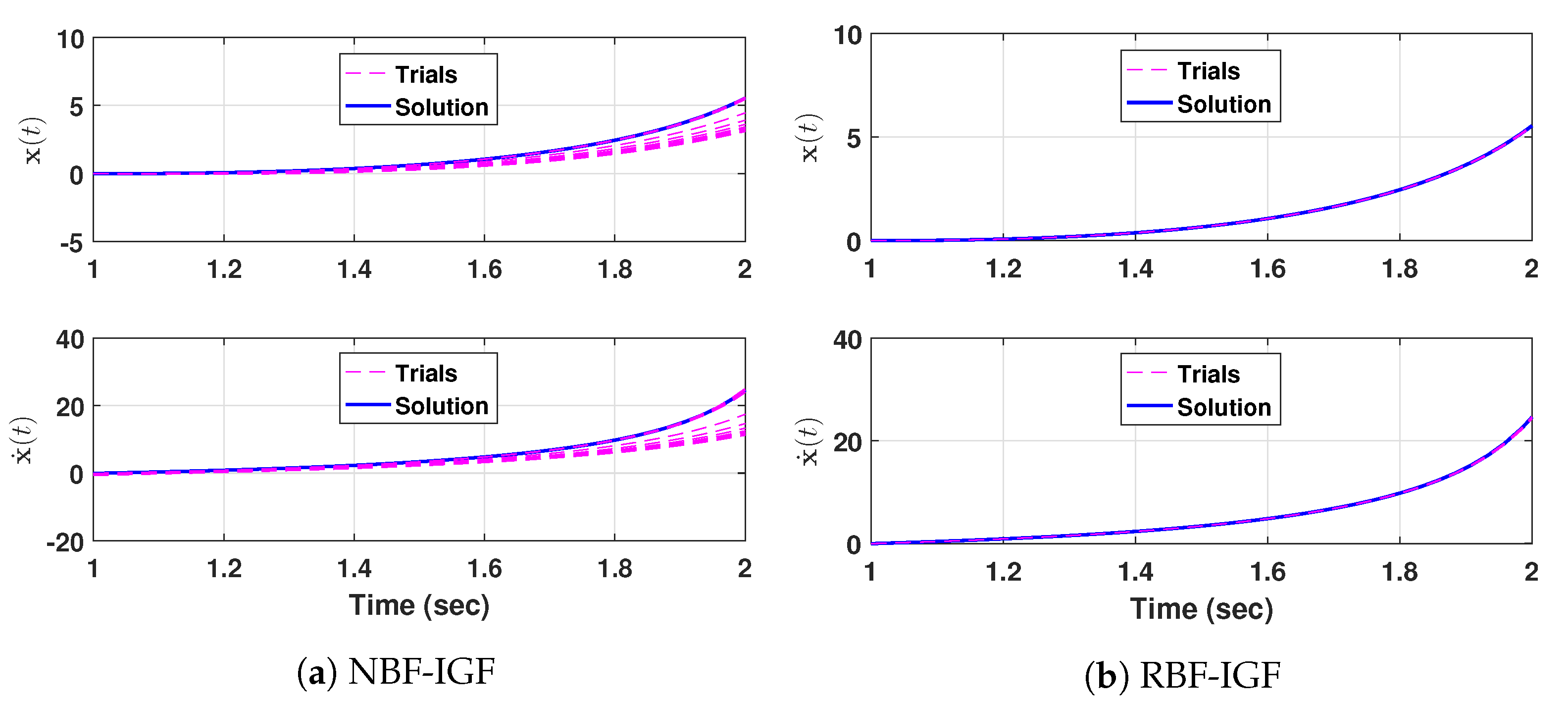
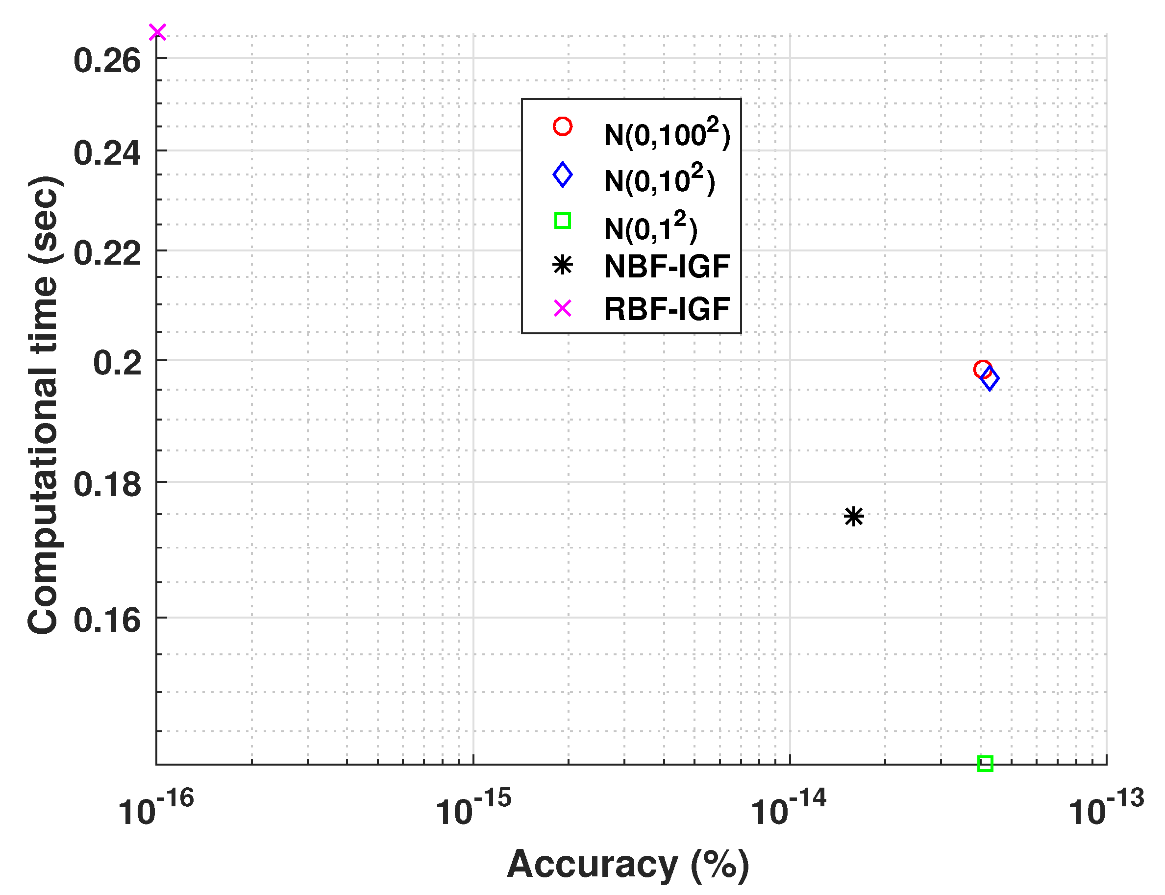
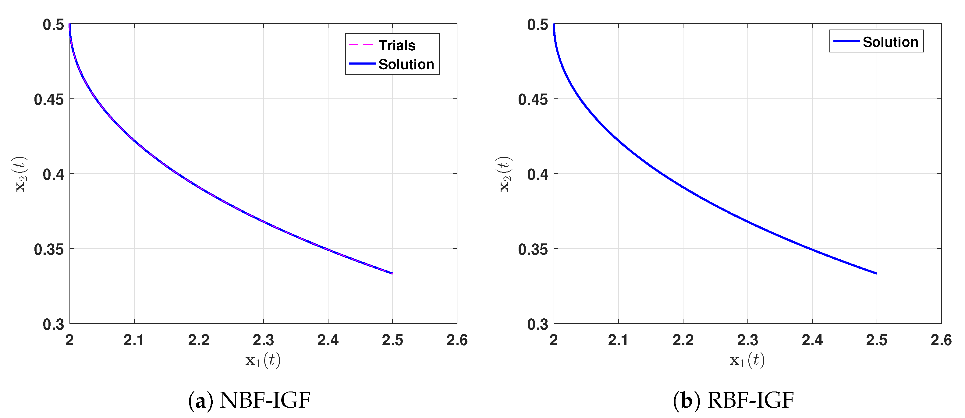
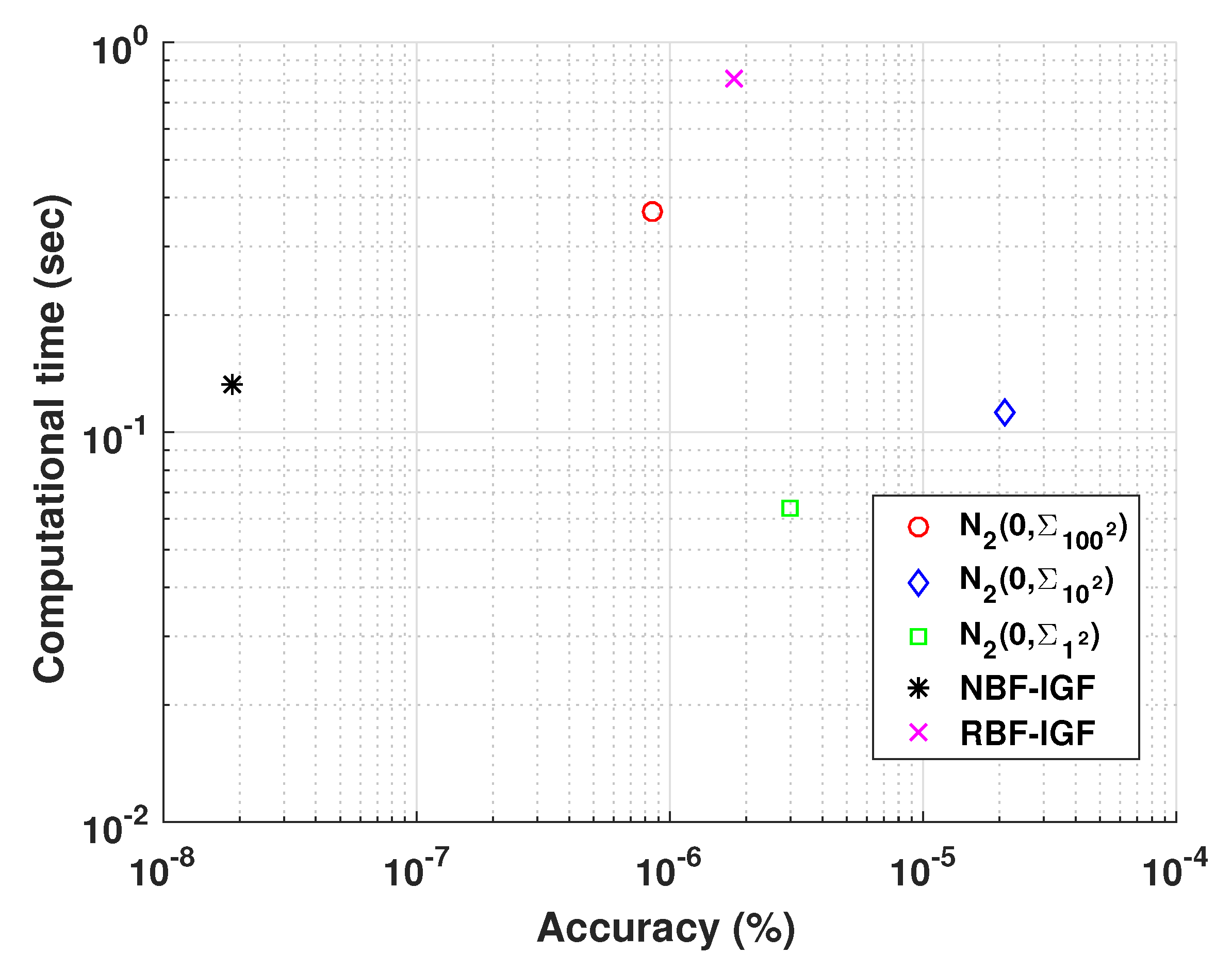
Note that the difference between the NBF-IGF and RBF-IGF arises in the first step that is the transformation of state variables, $t_B\left(s\right)$ and ${\mathbf{x}}_B\left(s\right)$, using Equations (2) and (5). Depending on the BFs, the number of unknown variables is different. Once the state variables are transformed into each BF, the following steps in Equations (14)–(17) remain the same. It is evident that the RBF-IGF provides a more accurate initial guess, because it has parametric flexibility that can more precisely approximate a curve. However, it is computationally more expensive than the NBF-IGF.

Subsequently, this problem becomes to solve Equation (17) with the unknown parameters and the following equations [25]:

$$\frac{\partial L}{\partial t_{B_i}}=0\mathrm{and}\frac{\partial L}{\partial {\mathbf{x}}_{B_i}}=\mathbf{0},$$

(18)

for $i=1,\cdots ,n-1$. Note that, if ${\mathit{f}}_B$ is made of products only in Equation (16), ${\mathit{g}}_B$ becomes a polynomial equation in s and Equation (17) can be solved in a closed form [25]. Once the obtained control points (and weights), which are the solution of the optimization problem, are applied to each state variable expressed as BFs, the approximated trajectory of the given BVP is found, and the initial guess for solving the given BVP is determined by ${\dot{\mathbf{x}}}_B{\left(s\right)|}_{s=0}$.

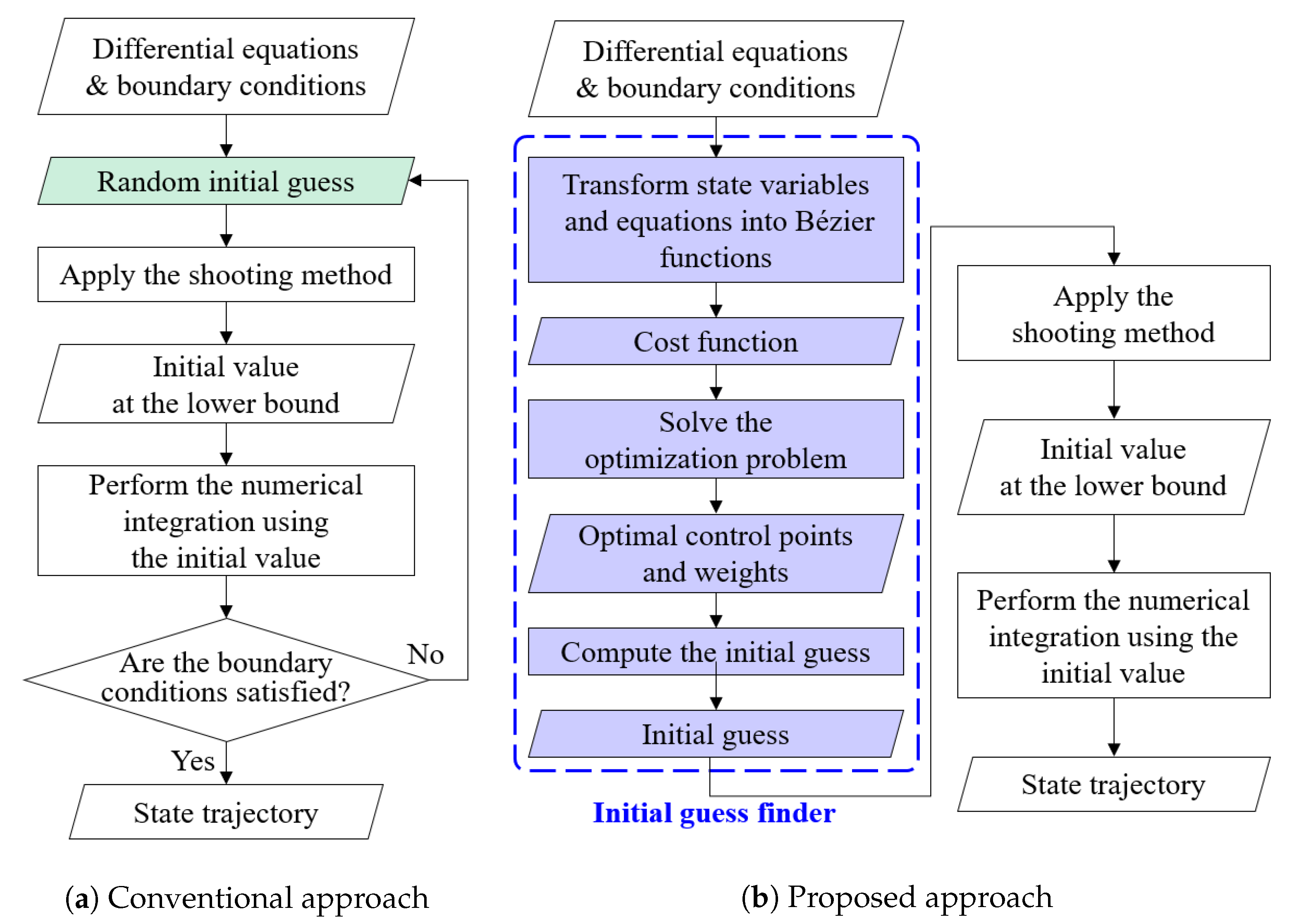
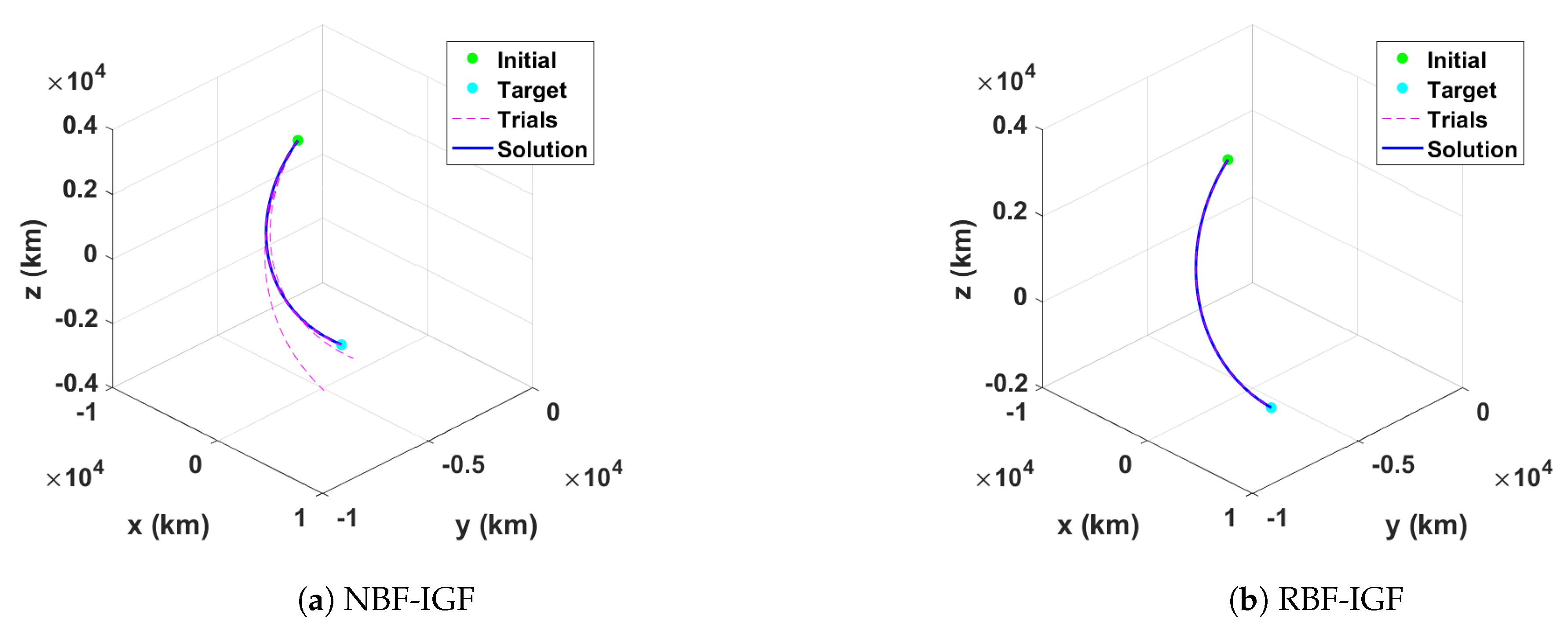
The given problem is generally solved by using the shooting method with random initial guesses because of the lack of information for the initial value, as shown in Figure 1a. If a proper initial guess is selected, then the shooting method provides the initial value for the lower bound that satisfies the given BCs. Subsequently, the numerical integration is performed by using the obtained initial value to find the solution, which is the state trajectory. If the BCs are not satisfied for the obtained state trajectory, different initial guesses should be selected. In fact, many engineering problems are sensitive to initial guesses, and this makes engineers spend a huge effort to find the proper initial guess. The IGFs that were proposed in this work provide a proper initial guess, even for the problems that are sensitive to initial guesses because the information of initial guess is based on the approximated trajectory for the given problem. Figure 1b shows the entire procedure for solving BVPs using the IGF that is highlighted with blue boxes. Initially, the state variables and equations are transformed into Bézier functions. Subsequently, the optimal control points and weights are obtained by solving the optimization problem that minimizes the cost function defined in Equation (17). Finally, using the obtained control points and weights, the initial guess is computed and applied to the shooting method. In fact, the initial value is relatively easily and efficiently found by using the initial guess that is provided by the proposed approach as compared to using random initial guesses. As shown in Figure 1a, the conventional approach iteratively selects random initial guesses to find the proper solution if the obtained states at the final time do not satisfy the BCs. On the other hand, replacing the green box shown in Figure 1a with the dashed blue box in Figure 1b eliminates such an iterative process.

3. Simulation Study

Numerical simulation studies are performed for several problems to validate the performance of the proposed IGF approaches. The shooting method is utilized to solve the given BVPs, and the simulation results using an initial guess obtained by each IGF are compared with the one using randomly selected initial guesses.

In the celestial mechanics, for example, the shape of the orbit trajectories is ellipse, parabola, or hyperbola, and a part of the entire elliptical orbit is generally the solution trajectory of Lambert’s problem. Therefore, the second order BFs can sufficiently approximate the orbital trajectory. Quadratic BFs are used in the simulation studies since the aim of this research is to find an initial guess to efficiently solve BVPs.

For the NBF-IGF, the quadratic NBFs and their first and second derivatives are given as

$$\begin{array}{ll}\hfill t_B\left(s\right)& ={(1-s)}^2{t}_{B_0}+2s(1-s)t_{B_1}+s^2{t}_{B_2},\hfill \\ \hfill t_B^{\prime }\left(s\right)& =2s(t_{B_2}-t_{B_1})+2(1-s)(t_{B_1}-t_{B_0}),\hfill \\ \hfill t_B^{″}\left(s\right)& =2(t_{B_0}-2t_{B_1}+t_{B_2}),\hfill \end{array}$$

(19)

$$\begin{array}{ll}\hfill x_{j,B}\left(s\right)& ={(1-s)}^2{x}_{j,B_0}+2s(1-s)x_{j,B_1}+s^2{x}_{j,B_2},\hfill \\ \hfill x_{j,B}^{\prime }\left(s\right)& =2s(x_{j,B_2}-x_{j,B_1})+2(1-s)(x_{j,B_1}-x_{j,B_0}),\hfill \\ \hfill x_{j,B}^{″}\left(s\right)& =2(x_{j,B_0}-2x_{j,B_1}+x_{j,B_2}),\hfill \end{array}$$

(20)

where $j=1,\cdots ,m$. Similarly, the quadratic RBFs and their first and second derivatives for the RBF-IGF are given as

$$\begin{array}{ll}\hfill t_B\left(s\right)& =\frac{w_{t_0}{(1-s)}^2{t}_{B_0}+2w_{t_1}(1-s)s{t}_{B_1}+w_{t_2}{s}^2{t}_{B_2}}{w_{t_0}{(1-s)}^2+2w_{t_1}(1-s)s+w_{t_2}{s}^2},\hfill \\ \hfill t_B^{\prime }\left(s\right)& =\frac{2s(w_{t_2}{t}_{B_2}-w_{t_1}{t}_{B_1})+2(1-s)(w_{t_1}{t}_{B_1}-w_{t_0}{t}_{B_0})-2(s(w_{t_2}-w_{t_1})-(1-s)(w_{t_1}-w_{t_0}))t_B\left(s\right)}{w_{t_0}{(1-s)}^2+2w_{t_1}(1-s)s+w_{t_2}{s}^2},\hfill \\ \hfill t_B^{″}\left(s\right)& =\frac{2(w_{t_2}{t}_{B_2}-2w_{t_1}{t}_{B_1}+w_{t_0}{t}_{B_0})-2(w_{t_2}-2w_{t_1}+w_{t_0})t_B-4(s(w_{t_2}-w_{t_1})-(1-s)(w_{t_1}-w_{t_0}))t_B^{\prime }\left(s\right)}{w_{t_0}{(1-s)}^2+2w_{t_1}(1-s)s+w_{t_2}{s}^2},\hfill \end{array}$$

(21)

$$\begin{array}{ll}\hfill x_{j,B}\left(s\right)& =\frac{w_{j,x_0}{(1-s)}^2{x}_{j,B_0}+2w_{j,x_1}(1-s)s{x}_{j,B_1}+w_{j,x_2}{s}^2{x}_{j,B_2}}{w_{j,x_0}{(1-s)}^2+2w_{j,x_1}(1-s)s+w_{j,x_2}{s}^2}\equiv \frac{x_{j,n}}{x_{j,d}},\hfill \\ \hfill x_{j,B}^{\prime }\left(s\right)& =\frac{x_{j,n}^{\prime }-x_{j,d}^{\prime }{x}_{j,B}\left(s\right)}{x_{j,d}},\hfill \\ \hfill x_{j,B}^{″}\left(s\right)& =\frac{x_{j,n}^{″}-x_{j,d}^{″}{x}_{j,B}-2x_{j,d}^{\prime }{x}_{j,B}^{\prime }\left(s\right)}{x_{j,d}},\hfill \end{array}$$

(22)

where

$$\begin{array}{ll}\hfill x_{j,n}^{\prime }& =2s(w_{j,x_2}{x}_{j,B_2}-w_{j,x_1}{x}_{j,B_1})+2(1-s)(w_{j,x_1}{x}_{j,B_1}-w_{j,x_0}{x}_{j,B_0}),\hfill \\ \hfill x_{j,n}^{″}& =2(w_{j,x_2}{x}_{j,B_2}-2w_{j,x_1}{x}_{j,B_1}+w_{j,x_0}{x}_{j,B_0}),\hfill \\ \hfill x_{j,d}^{\prime }& =2s(w_{j,x_2}-w_{j,x_1})+2(1-s)(w_{j,x_1}-w_{j,x_0}),\hfill \\ \hfill x_{j,d}^{″}& =2(w_{j,x_2}-2w_{j,x_1}+w_{j,x_0}).\hfill \end{array}$$

For the numerical studies, it considers 1D and 2D nonlinear BVPs, and then 3D nonlinear BVPs, in particular the orbit determination problems, are considered. For the shooting method, the bisection method [30,32] is used for the 1D example, because the 1D problem is identical to a root-finding problem. In the 2D and 3D examples, the trust-region algorithm [33] is utilized to solve systems of nonlinear equations. In addition to this, the simplex algorithm [34] is used to find the optimal control points and weights. These algorithms are run on Octave, which is free software, and the specifications of the computer for the simulation studies are as follows: Intel i7-7500U @ 2.7 GHz clock speed CPU and 12 GB memory.

3.1. Nonlinear 1D BVP

A nonlinear 1D BVP is given by [35]

$$\ddot{x}\left(t\right)=\frac{2{\dot{x}}^2\left(t\right)}{t^3}-\frac{9x^2\left(t\right)}{t^5}+4t,$$

(23)

where BCs are $x\left(t_{\mathrm{i}}=1\right)=0$ and $x\left(t_{\mathrm{f}}=2\right)=ln256$. At first, the given problem is solved using the shooting method with random initial guesses as the conventional approach. It considers three kinds of ranges for the initial guesses due to the lack of the initial value information and performing the Monte Carlo simulations with 1000 iterations for each range. Here, the initial guesses are randomly selected in the normal distribution (e.g., $\mathcal{N}\left(\mu ,{\sigma }^2\right)$, where $\mu$ is the mean and $\sigma$ is the standard deviation). The obtained initial value for each initial guess is displayed as the same value because the number obtained is the same up to the 14-th decimal place, as shown in

Table 1. Monte Carlo simulation results for 1D example using random initial guesses.

Initial Guess	$\mathcal{N}\left(0,{100}^2\right)$	$\mathcal{N}\left(0,{10}^2\right)$	$\mathcal{N}\left(0,1^2\right)$
Obtained initial value	−0.0751	−0.0751	−0.0751
Number of cases that found the solution	1000	1000	1000
Mean of number of iterations	28.0730	25.2150	20.7430
Mean of number of evaluations	40.0830	37.1640	32.5620
Mean of computational time (sec)	0.1986	0.1969	0.1408
Mean of $\left|x\left(t_{\mathrm{f}}\right)\right|$ error (%)	4.06 × 10${}^{-14}$	4.25 × 10${}^{-14}$	4.11 × 10${}^{-14}$

. Regardless of the initial guesses, it finds the solution with almost zero mean of the absolute error of $x\left(t_{\mathrm{f}}\right)$. Because the initial value to be obtained is near zero, the case for $\mathcal{N}\left(0,1^2\right)$ requires the least computational burden. Furthermore, it is easy to find the solution with an arbitrary initial guess, because the initial value to be obtained is scalar, not a vector in this problem.

Next, the proposed approach is applied to solve the given BVP. For this, the given equations are transformed into the quadratic NBFs and RBFs using Equations (19)–(22).

3.1.1. NBF-IGF

Because the endpoints are defined as $t_{B_0}(s=0)=1$, $t_{B_2}(s=1)=2$, $x_{B_0}(s=0)=0$, and $x_{B_2}(s=1)=ln256$, the number of unknown parameters is 2 (e.g., $t_{B_1}$ and $x_{B_1}$). Using Equation (16), the residual equation is transformed into

$$g_B={\ddot{x}}_B-f_B=\frac{x_B^{″}{t}_B^{\prime }-t_B^{″}{x}_B^{\prime }}{{t^{\prime }}_B^3}-\frac{2{(x_B^{\prime }/t_B^{\prime })}^2}{t_B^3}+\frac{9x_B^2}{t_B^5}-4t_B,$$

(24)

where each variable is defined in Equations (19) and (20). Because the given BVP should satisfy the zero residual, the approximated trajectory can be found as solving the optimization problem that minimizes the cost that is defined in Equation (17). Once the optimal intermediate control points are determined, the approximated solution trajectory over $s\in [0,1]$ is obtained, and the initial guess is easily computed at $s=0$ for Equation (14).

3.1.2. RBF-IGF

The endpoints are determined by the boundary values similar to NBF-IGF, and the weights that correspond to the endpoints are defined as 1 (i.e., $w_{t_0}=w_{t_2}=w_{1,x_0}=w_{1,x_2}=1$) as mentioned in Section 2.3. Therefore, the unknown variables are the intermediate control points and weights, and the number of unknowns is 4. By substituting the transformed variables and their derivatives in Equations (21) and (22) into Equation (24), the residual is obtained. Subsequently, the residual is applied to the cost function for the optimization problem in Equation (17). After solving the optimization problem, the initial guess is calculated by substituting the obtained control points and weights into Equation (14) at $s=0$.

In the optimization process, two kinds of stopping criteria are used: (i) the step size defined as the norm of the difference between the parameters at the current step and the previous step and (ii) the change in the value of the cost function during the current step and previous step. When both of the stopping criteria are satisfied, it terminates the optimization process provides the optimal control points and weights.

Table 2. Simulation results for 1D example by using the IGFs.

	NBF-IGF	RBF-IGF
Number of unknown parameters	2	4
Initial guess obtained by BFs	−0.7161	−0.0831
Obtained initial value	−0.0751	−0.0751
Number of iterations	18	9
Number of evaluations	29	14
Computational time (sec)	0.1746	0.2656
	(=0.1259 (B) + 0.0487 (S))	(=0.2448 (B) + 0.0209 (S))
$\left|x\left(t_{\mathrm{f}}\right)\right|$ error (%)	1.60 × 10${}^{-14}$	1.01 × 10${}^{-16}$

lists the initial guesses that are obtained by the proposed approaches and the corresponding simulation results applying the shooting method. Here, (B) represents the computational time for finding the control points and weights, and (S) means the computational time for performing the shooting method to find the proper initial value that satisfies the given BVP by using the initial guess obtained by the proposed approaches. The RBF-IGF provides the closer initial guess to the actual initial value than the NBF-IGF, because the RBFs have more flexibility (due to the additional weight parameters) than the NBFs. For this reason, a small number of iterations and evaluations is required to find the initial value that satisfies the given upper bound value with almost zero error. That is, the error is close to the machine epsilon value when applying the initial guess that is obtained from the RBF-IGF. Because the solution of the shooting method using the initial guess of the RBF-IGF is precisely computed, the obtained state at the upper bound is almost same as the given BC. It also explains that the trial trajectories of the shooting method using the initial guess obtained by the RBF-IGF are very close to the solution trajectory, as shown in Figure 2b, unlike the trial trajectories generated via the NBF-IGF shown in Figure 2a.

On the other hand, applying the initial guess that is obtained by the NBF-IGF into the shooting method is computationally more efficient than applying the other one because the NBF-IGF has only two unknown parameters to be optimized. In fact, the aim of this research is to provide an effective way to find the initial guess, not the actual initial value. For this reason, in between two IGFs, it can be said that the NBF-IGF is better to find the initial guess for solving the given BVP, because it is computationally inexpensive, and the initial guess is close enough to the initial value to be determined.

The IGF reduces a large amount of the computational time for applying the shooting method thanks to the properly selected initial guess, as shown in Table 1 and Table 2. When compared the computational time and the accuracy for the absolute value of the upper bound, the one using $\mathcal{N}\left(0,1^2\right)$ requires less computational time than the one that is required for the proposed approach, as shown in Figure 3, due to the fact that the initial value is close to zero.

However, it is shown that the NBF-IGF applied result provides better accuracy and less computational time overall.

3.2. Nonlinear 2D BVP

A nonlinear 2D BVP is given by [35]

$$\ddot{\mathbf{x}}\left(t\right)=\left[\begin{array}{c}{\ddot{x}}_1\left(t\right)\\ {\ddot{x}}_2\left(t\right)\end{array}\right]=\left[\begin{array}{c}2x_1^3\left(t\right)-3x_1\left(t\right)-2t^2\\ x_2^3\left(t\right)-x_2\left(t\right){\dot{x}}_2\left(t\right)\end{array}\right],$$

(25)

where $\mathbf{x}(t_{\mathrm{i}}=1)={[2,0.5]}^T$ and $\mathbf{x}(t_{\mathrm{f}}=2)={[2.5,1/3]}^T$. The given problem is first solved using the shooting method with random initial guesses, and the results are listed in

Table 3. Monte Carlo simulation results for 2D example using random initial guesses.

Initial Guess	${\mathcal{N}}_2(0,{\Sigma }_{{100}^2})$	${\mathcal{N}}_2(0,{\Sigma }_{{10}^2})$	${\mathcal{N}}_2(0,{\Sigma }_{1^2})$
Obtained initial value	[0, −0.25]${}^T$	[0, −0.25]${}^T$	[0, −0.25]${}^T$
Number of cases that found the solution	17	180	936
Mean of number of iterations	16.3529	11.0611	6.5139
Mean of number of evaluations	47.3529	33.2389	21.5908
Mean of computational time (sec)	0.3658	0.1130	0.0642
Mean of $\left|\right|\mathbf{x}\left(t_{\mathrm{f}}\right)\left|\right|$ error (%)	8.52 × 10${}^{-7}$	2.10 × 10${}^{-5}$	3.01 × 10${}^{-6}$

.

Here, ${\mathcal{N}}_m(\mathbf{\mu },{\Sigma }_{{\sigma }^2})$ indicates a m-dimensional normally-distributed random vector with the mean vector $\mathbf{\mu }\in {\mathbb{R}}^m$ and the covariance matrix ${\Sigma }_{{\sigma }^2}\in {\mathbb{R}}^{m\times m}$. In this work, the covariance matrix is defined as ${\Sigma }_{{\sigma }^2}={\sigma }^2{I}_{m\times m}$. Because the obtained initial value for each component is the same up to the 7-th decimal place, these values are displayed as the same values. Depending on the covariance of initial guesses, the number of cases that found the solution is differently obtained. In other words, this problem requires a proper initial guess to find the solution, unlike the 1D example. For the cases that found the solutions, the mean values, such as the mean of the number of iterations, number of evaluations, computational time, and upper bound norm error, are summarized in Table 3. That is, the cases that failed to find the solution are not included. The results show that the computational burden, such as the computational time and the number of iterations and evaluations, is reduced as the covariance of the initial guess decreases. In fact, these results are reasonable, because the initial guess of ${\mathcal{N}}_2(\mathbf{0},{\Sigma }_{1^2})$ is closer to the initial value obtained than the others.

Next, to apply the proposed approach, the variables and nonlinear functions for the given problem are transformed into the quadratic NBFs and RBFs while using Equations (19)–(22).

3.2.1. NBF-IGF

The given BCs are replaced with the endpoints as $t_{B_0}(s=0)=1,t_{B_2}(s=1)=2,{\mathbf{x}}_{B_0}(s=0)={[2,0.5]}^T$, and ${\mathbf{x}}_{B_2}(s=1)={[2.5,1/3]}^T$. Hence, three unknown control points are required to be determined, which are $t_{B_1}$ and ${\mathbf{x}}_{B_1}={[x_{1,B_1},x_{2,B_1}]}^T$. Using Equation (16), the residual and the nonlinear function on the right side of Equation (25) are transformed into the NBFs as

$${\mathit{g}}_B={\ddot{\mathbf{x}}}_B-{\mathit{f}}_B=\frac{{\mathbf{x}}_B^{″}{t}_B^{\prime }-t_B^{″}{\mathbf{x}}_B^{\prime }}{{t^{\prime }}_B^3}-\left[\begin{array}{c}2x_{1,B}^3-3x_{1,B}-2t_B^2\\ x_{2,B}^3-x_{2,B}(x_{2,B}^{\prime }/t_B^{\prime })\end{array}\right],$$

(26)

where each variable is defined in Equations (19) and (20), and the cost function is derived by substituting Equation (26) into Equation (17). Subsequently, the initial guess is obtained by using the same process of the 1D example.

3.2.2. RBF-IGF

The weights that correspond to the endpoints are set as $w_{t_0}=w_{t_2}=w_{{1,x}_0}=w_{{1,x}_2}=w_{{2,x}_0}=w_{{2,x}_2}=1$ similar to the 1D example. Therefore, six unknown variables, such as three control points and three weights ($w_{t_1}$ and ${\mathbf{w}}_{x_1}={[w_{1,x_1},w_{2,x_1}]}^T$), are considered. The residual is derived by applying the transformed variables and their derivatives in Equations (21) and (22) into Equation (26). The unknown variables are obtained by solving the optimization problem that minimizes the cost in Equation (17) composed of the residual, and the initial guess is computed by applying the obtained control points and weights into Equation (14) at $s=0$.

The results of the shooting method with the initial guesses obtained via the IGFs are listed in

Table 4. Simulation results for 2D example using the IGFs.

	NBF-IGF	RBF-IGF
Number of unknown parameters	3	6
Initial guess approximated by BFs	[1.4493 × 10${}^{-3}$, −2.4653 × 10${}^{-1}$]${}^T$	[−4.0795 × 10${}^{-5}$, −2.4992 × 10${}^{-1}$]${}^T$
Obtained initial value	[−9.4189 × 10${}^{-9}$, −2.5000 × 10${}^{-1}$]${}^T$	[1.3005 × 10${}^{-8}$, −2.5000 × 10${}^{-1}$]${}^T$
Number of iterations	2	1
Number of evaluations	9	6
Computational time (sec)	0.1319	0.8024
	(=0.1027 (B) + 0.0290 (S))	(=0.7802 (B) + 0.0222 (S))
$\left|\right|\mathbf{x}\left(t_{\mathrm{f}}\right)\left|\right|$ error (%)	1.88 × 10${}^{-8}$	1.79 × 10${}^{-6}$

. The initial guess generated via the NBF-IGF finds the initial value after one trial shown in Figure 4a. On the other hand, the initial guess that is obtained by the RBF-IGF requires only one iteration to find the initial value. Because the RBFs provided the closer initial guess to the initial value, no trial trajectory is required, especially for this example, as shown in Figure 4b.

On the other hand, applying the NBF-IGF provides a huge benefit in the aspect of the computational efficiency. In addition to this, the upper bound norm error is obtained as a very small value that is close to zero. Similar to the 1D example, it can be said that the NBF-IGF is the better approach than the RBF-IGF.

Both IGFs provide suitable initial guesses and, thus, the shooting method finds the solution for the given problem with the small number of iterations, whereas the conventional approach sometimes fails to find the solutions, as shown in Table 3 and Table 4. In particular, applying the random initial guess with ${\mathcal{N}}_2\left(\mathbf{0},{\Sigma }_{{100}^2}\right)$ provides a poor success rate that finds the solution. In addition, Figure 5 shows that the accuracy of the upper bound norm error and the computational time when using random initial guesses and the initial guess that was obtained by the IGFs.

It is shown that the shooting method with the NBF-IGF is superior in the aspect of considering both computational cost and accuracy simultaneously.

3.3. Nonlinear 3D BVP: Orbit Determination Applications

Lambert’s problem is one of the popular nonlinear BVPs in the celestial mechanics with 3D space. The two-body equation is given by [36]

$$\ddot{\mathbf{r}}\left(t\right)=-\frac{\mu }{{\left|\right|\mathbf{r}\left(t\right)\left|\right|}^3}\mathbf{r}\left(t\right),$$

(27)

that satisfies $\mathbf{r}\left(t_{\mathrm{i}}\right)={\mathbf{r}}_{\mathrm{i}}$ and $\mathbf{r}\left(t_{\mathrm{f}}\right)={\mathbf{r}}_{\mathrm{f}}$. Here, $\mathbf{r}\left(t\right)\in {\mathbb{R}}^3$ is the position vector, $\mu$ is the gravitational coefficient, which is defined as $\mu =398,600$ km${}^3/$sec${}^2$, $\left|\right|\mathbf{r}\left(t\right)\left|\right|$ is the magnitude of the position vector, and ${\mathbf{r}}_{\mathrm{i}}$ and ${\mathbf{r}}_{\mathrm{f}}$ are the initial and final position vectors, respectively.

The performance of the proposed approaches for the orbit determination problem is validated by considering three orbits that have different semi-major axes and eccentricities, and they are listed in

Table 5. Orbits information considered in simulations.

Orbit	Semi-Major Axis	Eccentricity
Hubble telescope orbit	6917 km	0.000283
Tundra orbit	42,164 km	0.268
Molniya orbit	26,600 km	0.74

.

In the orbit determination problem, the initial velocity at the initial time is found by applying the shooting method. Because each orbit has a different initial velocity, depending on the initial position, three kinds of initial positions are considered to deal with various initial velocities: near apogee, intermediate (between the apogee and perigee), and near perigee. Note that only one initial position is considered for Hubble telescope orbit, because it is almost circular orbit.

Table 6. Simulation parameters for the 3D example.

	${\mathit{t}}_{\mathbf{f}}$ (sec)	${\mathbf{r}}_{\mathbf{i}}$ (km)	${\mathbf{r}}_{\mathbf{f}}$ (km)
Hubble	1500	[−5641.48, −3331.74, 2204.25]${}^T$	[3329.05, −5754.98, −871.62]${}^T$
Tundra (apogee)	25,000	[15,040.51, 22,615.10, 45,161.32]${}^T$	[−36,285.49, 13,559.48, 27,077.65]${}^T$
Tundra (intermediate)	15,000	[−40,292.40, 7484.69, 14,946.57]${}^T$	[−17,983.49, −11,870.23, −23,704.31]${}^T$
Tundra (perigee)	17,000	[−24,501.90, −9999.97, −19,969.49]${}^T$	[33,647.42, −5531.99, −11,047.13]${}^T$
Molniya (apogee)	18,000	[7062.08, 19,756.30, 39,452.43]${}^T$	[−16,831.22, 12,838.49, 25,637.87]${}^T$
Molniya (intermediate)	5000	[−17,436.33, 11,461.54, 22,888.17]${}^T$	[−14,505.52, 1846.23, 3686.84]${}^T$
Molniya (perigee)	5000	[−3653.53, −2884.55, −5680.43]${}^T$	[17,638.45, 6821.86, 13,622.94]${}^T$

lists the BCs for each orbit. Here, the initial time $t_{\mathrm{i}}$ is set as zero, so only the final time information is given.

Initially, the shooting method with random initial guesses is applied to all cases, and

Table 7. Monte Carlo simulation results for 3D example using random initial guesses.

	Hubble	Tundra			Molniya
		Apogee	Intermediate	Perigee	Apogee	Intermediate	Perigee
Number of cases that found the solution	714	659	850	734	856	978	0
Mean of number of iterations	9.0686	9.0030	8.7576	11.4659	8.6472	7.5542	-
Mean of number of evaluations	39.2199	39.6748	38.5471	47.0150	38.1822	34.1769	-
Mean of computational time (sec)	1.2779	8.2786	5.0861	7.0179	5.7960	1.5298	-
Mean of $\left|\right|{\mathbf{r}}_{\mathrm{f}}\left|\right|$ error (%)	2.44 × 10${}^{-3}$	3.70 × 10${}^{-3}$	2.45 × 10${}^{-3}$	3.62 × 10${}^{-2}$	1.61 × 10${}^{-3}$	5.25 × 10${}^{-5}$	-

lists the Monte Carlo simulation results (1000 iterations) for each orbit case. Note that the initial guesses are randomly generated as ${\mathcal{N}}_3\left(\mathbf{0},{\Sigma }_{{10}^2}\right)$, because the speed at each position is around 1.5∼10 km/sec. It sometimes fails to find the solution and, in particular, no solution is found for the near perigee case of Molniya orbit, as shown in the table. Because the initial value at the lower bound for the near perigee of Molniya orbit is relatively greater than the other cases, it is critical to an initial guess in order to find the solution. Like the 2D example, the cases that found the solution are only considered to compute the mean values of the number of iterations, the number of evaluations, computational time, and the upper bound norm error. Once the solution is found, the upper bound norm error is achieved as less than 0.05 %, and the solution is well found. However, one can say that the random initial guesses do not guarantee to find the solution, as shown in Table 7.

To apply the proposed approach into this problem, four variables, which are the time t, and three components of the position vector $\mathbf{r}\left(t\right)$, are transformed into the quadratic NBFs and RBFs using Equations (19)–(22).

3.3.1. NBF-IGF

For the given BCs that are listed in Table 6, the endpoints for each case are defined for the NBFs, like the previous examples, and this problem has four unknown control points ($t_{B_1}$ and ${\mathbf{r}}_{B_1}={[r_{1,B_1},r_{2,B_1},r_{3,B_1}]}^T$). The residual, including the nonlinear function on the right side of Equation (27), is derived as

$${\mathit{g}}_B={\ddot{\mathbf{r}}}_B-{\mathit{f}}_B=\frac{{\mathbf{r}}_B^{″}{t}_B^{\prime }-t_B^{″}{\mathbf{r}}_B^{\prime }}{{t^{\prime }}_B^3}-\frac{\mu }{\left|\right|{\mathbf{r}}_B{\left|\right|}^3}{\mathbf{r}}_B,$$

(28)

and the variables are defined in Equations (19) and (20). After applying the residual in Equation (28) into the cost function in Equation (17) and solving the optimization problem, the initial guess is computed using the obtained control points at $s=0$.

3.3.2. RBF-IGF

The endpoints are defined as the same way of the NBF-IGF, and the weights that are associated with the endpoints are defined as $w_{t_0}=w_{t_2}=w_{1,r_0}=w_{1,r_2}=w_{2,r_0}=w_{2,r_2}=w_{3,r_0}=w_{3,r_2}=1$. Hence, the number of unknown parameters is eight: four control points and four weights that are defined as $t_{B_1}$, ${\mathbf{r}}_{B_1}$, $w_{t_1}$, and ${\mathbf{w}}_{r_1}={[w_{1,r_1},w_{2,r_1},w_{3,r_1}]}^T$. With these unknown parameters, the cost function in Equation (17) is derived using Equation (28). The unknown intermediate control points and weights are obtained by solving the optimization problem, and the initial guess is calculated by applying the obtained parameters into Equation (14) at $s=0$.

Using the simulation parameters that are listed in Table 6, the numerical simulations for the proposed approaches are conducted, and

Table 8. The simulation results for Hubble telescope orbit using the IGFs.

	NBF-IGF	RBF-IGF
Number of unknown parameters	4	8
Initial guess by BFs	[4.4958, −7.4692, −2.5057]${}^T$	[3.1892, −6.6256, −1.8750]${}^T$
Obtained initial value	[3.1883, −6.6303, −1.8752]${}^T$	[3.1883, −6.6303, −1.8752]${}^T$
Number of iterations	5	3
Number of evaluations	24	16
Computational time (sec)	0.7423	1.4350
	(= 0.2384 (B) + 0.5039 (S))	(= 1.1623 (B) + 0.2727 (S))
$\left|\right|{\mathbf{r}}_{\mathrm{f}}\left|\right|$ error (%)	8.17 × 10${}^{-5}$	8.17 × 10${}^{-5}$

,

Table 9. Simulation results for Tundra orbit (apogee) using the IGFs.

	NBF-IGF	RBF-IGF
Number of unknown parameters	4	8
Initial guess approximated by BFs	[−2.6141, 0.3707 −0.7402]${}^T$	[−2.2044, 0.4068, 0.8122]${}^T$
Obtained initial value	[−2.2024, −0.4074, 0.8136]${}^T$	[−2.2024, −0.4074, 0.8136]${}^T$
Number of iterations	4	3
Number of evaluations	20	16
Computational time (sec)	4.0855	4.4808
	(= 0.1772 (B) + 3.9083 (S))	(= 1.0031 (B) + 3.4777 (S))
$\left|\right|{\mathbf{r}}_{\mathrm{f}}\left|\right|$ error (%)	2.26 × 10${}^{-5}$	2.26 × 10${}^{-5}$

,

Table 10. Simulation results for Tundra orbit (intermediate) using the IGFs.

	NBF-IGF	RBF-IGF
Number of unknown parameters	4	8
Initial guess approximated by BFs	[−0.2581, −1.6221, −3.2393]${}^T$	[−0.3542, −1.3209, −2.6377]${}^T$
Obtained initial value	[−0.3669, −1.3200, −2.6360]${}^T$	[−0.3669, −1.3200, −2.6360]${}^T$
Number of iterations	4	3
Number of evaluations	20	16
Computational time (sec)	2.8944	3.4718
	(= 0.2739 (B) + 2.6205 (S))	(= 1.4237 (B) + 2.2048 (S))
$\left|\right|{\mathbf{r}}_{\mathrm{f}}\left|\right|$ error (%)	1.55 × 10${}^{-5}$	1.55 × 10${}^{-5}$

,

Table 11. Simulation results for Tundra orbit (perigee) using the IGFs.

	NBF-IGF	RBF-IGF
Number of unknown parameters	4	8
Initial guess approximated by BFs	[3.9257, −1.1812, −2.3588]${}^T$	[3.0000, −1.0583, −2.1134]${}^T$
Obtained initial value	[3.0053, −1.0563, −2.1093]${}^T$	[3.0053, −1.0563, −2.1093]${}^T$
Number of iterations	4	3
Number of evaluations	20	16
Computational time (sec)	3.1469	3.8489
	(= 0.2589 (B) + 2.8880 (S))	(= 1.6548 (B) + 2.1941 (S))
$\left|\right|{\mathbf{r}}_{\mathrm{f}}\left|\right|$ error (%)	7.54 × 10${}^{-4}$	7.54 × 10${}^{-4}$

,

Table 12. Simulation results for Molniya orbit (apogee) using the IGFs.

	NBF-IGF	RBF-IGF
Number of unknown parameters	4	8
Initial guess approximated by BFs	[−1.7511, 0.3576, 0.7140]${}^T$	[−1.4359, 0.4058, 0.8103]${}^T$
Obtained initial value	[−1.4240, 0.4070, 0.8129]${}^T$	[−1.4240, 0.4070, 0.8129]${}^T$
Number of iterations	4	3
Number of evaluations	20	16
Computational time (sec)	2.9211	3.2541
	(= 0.1543 (B) + 2.7668 (S))	(= 1.0329 (B) + 2.2212 (S))
$\left|\right|{\mathbf{r}}_{\mathrm{f}}\left|\right|$ error (%)	8.49 × 10${}^{-6}$	8.49 × 10${}^{-6}$

,

Table 13. Simulation results for Molniya orbit (intermediate) using the IGFs.

	NBF-IGF	RBF-IGF
Number of unknown parameters	4	8
Initial guess approximated by BFs	[−0.7146, −1.5981, −3.1913]${}^T$	[−0.4975, −1.4518, −2.8991]${}^T$
Obtained initial value	[−0.4975, −1.4513, −2.8981]${}^T$	[−0.4975, −1.4513, −2.8981]${}^T$
Number of iterations	3	2
Number of evaluations	16	12
Computational time (sec)	0.8887	1.4315
	(= 0.1816 (B) + 0.7071 (S))	(= 0.8740 (B) + 0.5575 (S))
$\left|\right|{\mathbf{r}}_{\mathrm{f}}\left|\right|$ error (%)	2.35 × 10${}^{-6}$	2.35 × 10${}^{-6}$

and

Table 14. Simulation results for Molniya orbit (perigee) using the IGFs.

	NBF-IGF	RBF-IGF
Number of unknown parameters	4	8
Initial guess approximated by BFs	[7.8363, 2.4444, −4.8819]${}^T$	[8.9313, −1.4052, −2.8067]${}^T$
Obtained initial value	[9.2497, −1.2852, −2.5665]${}^T$	[9.2497, −1.2852, −2.5665]${}^T$
Number of iterations	6	4
Number of evaluations	28	20
Computational time (sec)	2.2736	3.4960
	(= 0.2713 (B) + 2.0023 (S))	(= 2.5954 (B) + 0.9006 (S))
$\left|\right|{\mathbf{r}}_{\mathrm{f}}\left|\right|$ error (%)	8.70 × 10${}^{-2}$	8.70 × 10${}^{-2}$

summarize the results. Overall, the proposed approaches provide the solution with less than 0.1% upper bound norm errors. Similar to the 1D and 2D examples, applying the RBF-IGF provides a closer initial guess to the initial value, and the shooting method with the RBF-IGF requires a less number of iterations and evaluations to find the solution. Because the initial guess is very close to the initial value, the trial trajectories are also similar to the solution trajectory, as shown in Figure 6, Figure 7 and Figure 8.

However, the NBF-IGF also provides an initial guess that is close enough to the initial value to be obtained and it requires less computational time to obtain the initial guess and find the solution with the shooting method. Furthermore, the obtained upper bound norm error using the NBF-IGF is the same as the one using the RBF-IGF. Therefore, one can be said that that the NBF-IGF has better performance than the RBF-IGF in between both of the IGFs proposed.

Although the shooting method with random initial guesses provides the solution over 65 % during 1000 times simulations, except for the near perigee case of Molniya orbit, this does not guarantee finding the solution. On the other hand, the proposed approaches find the solution for all cases, including the near perigee case of Molniya orbit. In addition, applying the IGF, especially the NBF-IGF, guarantees the least computational burden to find the solution than the others, as shown in Figure 9.

Here, “Conventional” indicates the shooting method with random initial guesses, and the numbers shown in Figure 9 represent the computational time. Therefore, it is concluded that the proposed IGFs are able to provide suitable initial guesses that guarantee finding the solution of the orbit determination problem, including the case that is sensitive to the initial guess. Because the NBF-IGF not only provides an initial guess close to the initial value, but is also computationally more efficient than the RBF-IGF, the NBF-IGF is more beneficial than the RBF-IGF to determine the initial guess.

4. Conclusions

This work proposes efficient initial guess finders (IGFs) that provide proper initial guesses as approximating BVPs by using the non-rational and rational Bézier functions (BFs). Each IGF is named NBF-IGF and RBF-IGF, respectively. The IGFs provided proper initial guesses at the lower bound, and this value is applied to the shooting method. To validate the efficacy of the proposed approach, various dimensional problems from one-dimensional (1D) to 3D, including Lambert’s problem, are studied and compared with the conventional shooting method. For the 1D and 2D problems, the IGFs are as good as the conventional approach that uses random initial guesses, because the problems are relatively easy to solve. On the other hand, for the 3D Lambert’s problem, the proposed IGFs outperform the conventional approach in terms of the computational burden and the ability to find the solution. In between two IGFs, although the RBF-IGF provides a more accurate initial guess, the NBF-IGF provides a close enough initial guess and it requires less computational burden. Therefore, the NBF-IGF is a better option than the RBF-IGF for providing a proper initial guess to effectively solve the BVPs.

References

1. Battin, R. An Introduction to the Mathematics and Methods of Astrodynamics; AIAA Education Series; American Institute of Aeronautics and Astronautics: New York, NY, USA, 1987. [Google Scholar]
2. Leeghim, H.; Jaroux, B.A. Energy-Optimal Solution to the Lambert Problem. J. Guid. Control Dyn. 2010, 33, 1008–1010. [Google Scholar] [CrossRef]
3. Oghim, S.; Leeghim, H.; Kim, D. Real-time spacecraft intercept strategy on J2-perturbed orbits. Adv. Space Res. 2019, 63, 1007–1016. [Google Scholar] [CrossRef]
4. Oghim, S.; Mok, S.H.; Leeghim, H. Optimal spacecraft rendezvous by minimum velocity change and wait time. Adv. Space Res. 2017, 60, 1188–1200. [Google Scholar] [CrossRef]
5. Baranov, A.; Grishko, D.; Khukhrina, O.; Chen, D. Optimal transfer schemes between space debris objects in geostationary orbit. Acta Astronaut. 2020, 169, 23–31. [Google Scholar] [CrossRef]
6. Bézier, P.E. Définition Numérique des Courbes et Surfâces I. Automatisme 1966, XI, 625–632. [Google Scholar]
7. Bézier, P.E. Définition Numérique des Courbes et Surfâces II. Automatisme 1967, XII, 17–21. [Google Scholar]
8. Bézier, P.E. Procédé de Définition Numérique des Courbes et Surfâces non Mathématiques. Automatisme 1968, XIII, 189–196. [Google Scholar]
9. Chen, W.; Chiu, K.; Fuge, M.D. Airfoil Design Parameterization and Optimization Using Bézier Generative Adversarial Networks. AIAA J. 2020, 58, 4723–4735. [Google Scholar] [CrossRef]
10. Fowler, L.; Rogers, J. Bézier Curve Path Planning for Parafoil Terminal Guidance. J. Aerosp. Inf. Syst. 2014, 11, 300–315. [Google Scholar] [CrossRef] [Green Version]
11. Ingersoll, B.T.; Ingersoll, J.K.; DeFranco, P.; Ning, A. UAV Path-Planning using Bezier Curves and a Receding Horizon Approach. In Proceedings of the AIAA Modeling and Simulation Technologies Conference, Washington, DC, USA, 13–17 June 2016; pp. 1–14. [Google Scholar] [CrossRef] [Green Version]
12. Manyam, S.G.; Casbeer, D.; Weintraub, I.E.; Tran, D.M.; Bradley, J.M.; Darbha, S. Quadratic Bezier Curves for Multi-Agent Coordinated Arrival in the Presence of Obstacles. In Proceedings of the AIAA Scitech 2021 Forum, Virtual, 11–15 & 19–21 January 2021; pp. 1–8. [Google Scholar] [CrossRef]
13. Miller, A.; Walczak, S. Maritime Autonomous Surface Ship’s Path Approximation Using Bézier Curves. Symmetry 2020, 12, 1704. [Google Scholar] [CrossRef]
14. Satai, H.A.; Zahra, M.M.A.; Rasool, Z.I.; Abd-Ali, R.S.; Pruncu, C.I. Bézier Curves-Based Optimal Trajectory Design for Multirotor UAVs with Any-Angle Pathfinding Algorithms. Sensors 2021, 21, 2460. [Google Scholar] [CrossRef]
15. Lattarulo, R.; Pérez Rastelli, J. A Hybrid Planning Approach Based on MPC and Parametric Curves for Overtaking Maneuvers. Sensors 2021, 21, 595. [Google Scholar] [CrossRef]
16. Mehdi, S.B.; Choe, R.; Hovakimyan, N. Piecewise Bézier Curves for Avoiding Collisions During Multivehicle Coordinated Missions. J. Guid. Control Dyn. 2017, 40, 1567–1578. [Google Scholar] [CrossRef]
17. Mehdi, S.B.; Choe, R.; Hovakimyan, N. Collision Avoidance in Cooperative Missions: Bézier Surfaces for Circumnavigating Uncertain Speed Profiles. J. Guid. Control Dyn. 2019, 42, 1779–1796. [Google Scholar] [CrossRef]
18. Scoccia, C.; Palmieri, G.; Palpacelli, M.C.; Callegari, M. A Collision Avoidance Strategy for Redundant Manipulators in Dynamically Variable Environments: On-Line Perturbations of Off-Line Generated Trajectories. Machines 2021, 9, 30. [Google Scholar] [CrossRef]
19. Abdelaal, M.; Schön, S. Predictive Path Following and Collision Avoidance of Autonomous Connected Vehicles. Algorithms 2020, 13, 52. [Google Scholar] [CrossRef] [Green Version]
20. Choe, R.; Puig-Navarro, J.; Cichella, V.; Xargay, E.; Hovakimyan, N. Cooperative Trajectory Generation Using Pythagorean Hodograph Bézier Curves. J. Guid. Control Dyn. 2016, 39, 1744–1763. [Google Scholar] [CrossRef]
21. Dilectis, F.D.; Mortari, D.; Zanetti, R. Bézier Description of Space Trajectories. J. Guid. Control Dyn. 2016, 39, 2535–2539. [Google Scholar] [CrossRef] [Green Version]
22. Pan, B.; Ma, Y. Lambert’s Problem and Solution By Non-Rational Bézier Functions. Proc. Inst. Mech. Eng. Part G J. Aerosp. Eng. 2018, 232, 227–245. [Google Scholar] [CrossRef]
23. Mortari, D.; Clocchiatti, A. Solving Kepler’s Equation Using Bézier Curves. Celest. Mech. Dyn. Astron. 2007, 99, 45–57. [Google Scholar] [CrossRef]
24. Mortari, D.; Elipe, A. Solving Kepler’s Equation Using Implicit Functions. Adv. Astronaut. Sci. 2014, 150, 389–399. [Google Scholar] [CrossRef]
25. Kim, D.; Mortari, D. Applications of Implicit Functions To Orbital Me/chanics Problems. In Proceedings of the 24th AAS/AIAA Spaceflight Mechanics Meeting, Santa Fe, NM, USA, 26–30 January 2014; pp. 1–12. [Google Scholar]
26. Bernstein, S.N. Collected Works; Acad. Nauk. SSSR: Moscow, Russia, 1952; Volume 1, pp. 105–106. [Google Scholar]
27. Bernstein, S.N. Collected Works; Acad. Nauk. SSSR: Moscow, Russia, 1954; Volume 2, pp. 310–348. [Google Scholar]
28. Marsh, D. Applied Geometry for Computer Graphics and CAD; Springer Undergraduate Mathematics Series; Springer: Berlin/Heidelberg, Germany, 1999. [Google Scholar]
29. Farin, G. Curves and Surfaces for CAGD: A Practical Guide, 5th ed.; Morgan Kaufmann Publishers: San Francisco, CA, USA, 2002. [Google Scholar]
30. Burden, R.L.; Faires, D.J.; Burden, A.M. Numerical Analysis, 10th ed.; Cengage Learning: Boston, MA, USA, 2014. [Google Scholar]
31. Choi, D.; Yang, S.; Leeghim, H.; Kim, D. A Study on Effective Initial Guess Finding Method Based on Bézier Curves: Orbit Determination Applications. In Proceedings of the 2019 AAS/AIAA Astrodynamics Specialist Conference, Portland, ME, USA, 11–15 August 2019; pp. 2651–2660. [Google Scholar]
32. Brent, R. Algorithms for Minimization without Derivatives; Prentice-Hall: Englewood Cliffs, NJ, USA, 1973. [Google Scholar]
33. Coleman, T.F.; Li, Y. An Interior Trust Region Approach for Nonlinear Minimization Subject to Bounds. SIAM J. Optim. 1996, 6, 418–445. [Google Scholar] [CrossRef] [Green Version]
34. Lagarias, J.C.; Reeds, J.A.; Wright, M.H.; Wright, P.E. Convergence Properties of the Nelder–Mead Simplex Method in Low Dimensions. SIAM J. Optim. 1998, 9, 112–147. [Google Scholar] [CrossRef] [Green Version]
35. Keskin, A.U. Boundary Value Problems for Engineers: With MATLAB Solutions; Springer International Publishing: Berlin/Heidelberg, Germany, 2019. [Google Scholar]
36. Schaub, H.; Junkins, J. Analytical Mechanics of Space Systems; AIAA Education Series; American Institute of Aeronautics and Astronautics: Reston, VA, USA, 2009. [Google Scholar] [CrossRef]
Figure 1. Flowchart for solving BVPs.
Symmetry 13 00736 g001
Figure 2. State trajectories for trials and the solution.
Symmetry 13 00736 g002
Figure 3. Accuracy vs. computational time comparison for 1D example.
Symmetry 13 00736 g003
Figure 4. Phase trajectories for trials and the solution.
Symmetry 13 00736 g004
Figure 5. Accuracy vs. computational time comparison for 2D example.
Symmetry 13 00736 g005
Figure 6. State trajectories of trials and the solution for 3D example: Hubble telescope orbit.
Symmetry 13 00736 g006
Figure 7. State trajectories of trials and the solution for 3D example: Tundra orbit.
Symmetry 13 00736 g007
Figure 8. State trajectories of trials and the solution for 3D example: Molniya orbit.
Symmetry 13 00736 g008
Figure 9. Computational time comparisons for 3D example.
Symmetry 13 00736 g009