Abstract
This paper presents a novel approach for an Intrusion Detection System (IDS) based on one kind of asymmetric optimization which use any three already well-known IDS algorithms and Triple Modular Redundancy (TMR) algorithm together. Namely, a variable threshold which indicates an attack on an observed and protected network is determined by using all three values obtained with three known IDS algorithms i.e., on previously recorded data by making a decision by majority. For these algorithms authors used algorithm of k-nearest neighbors, cumulative sum algorithm, and algorithm of exponentially weighted moving average. Using a proposed method we can get a threshold that is more precisely determined than in the case of any method individual. Practically, using TMR we obtain a dynamically threshold adjustment of IDS software, which reduces the existence of false alarms and undetected attacks, so the efficiency of such IDS software is notably higher and can get better results. Today, Denial of Service attacks (DoS) are one of the most present type of attacks and the reason for the special attention paid to them in this paper. In addition, the authors of the proposed method for IDS software used a known CIC-DDoS2019 dataset, which contains various data recordings of such attacks. Obtained results with the proposed solution showed better characteristics than each individual used algorithm in this solution. IDS software with the proposed method worked precisely and timely, which means alarms were triggered properly and efficiently.
1. Introduction
Today, IT security is one of the most important questions for professionals, corporations, governments, etc. As IT technologies grow rapidly and constantly, we cannot imagine our life without them. Security risks have never been higher than they are today, all because technology and the internet are available to almost half of Earth’s population. Everybody has a mobile phone, smartwatch, tablet, PC—or at least one of those and most of them are unprotected while going online.
Pertaining to corporations, along with governmental and non-governmental bodies, IT security is somewhat improved, but is commonly not adequate or even non-existent. Governments nowadays have their own Computer Emergency Response Team (CERT) that handles attacks and security incidents, while private companies have their in-house IT security departments, or they hire a professional to organize IT security protection for them—so-called outsourcing. Even with these measures to prevent security incidents, it is still possible to sustain attacks and security breaches that can create a lot of damage.
Distributed Denial of Service (DDoS) as well Denial of Service (DoS) attacks are the most common kind of attacks, and also the biggest problem if proper protection is not enabled inside a targeted system. A DDoS attack is a large number of requests from different hosts and attempts to exceed the limit of the network that is the target of attack. It is usually distributed by a previously infected large number of computers or other internet-connected devices, so-called bot-net networks. Choosing the right way to detect these attacks [1,2] is a big challenge as they come in different forms, like flood attacks, protocol attacks, and application-layer attacks [3,4]. In this paper, we focus on flood attacks, like Hypertext Transfer Protocol (HTTP) flood and User Datagram Protocol (UDP) flood attacks. DDoS and DoS attacks are mostly the same thing, the difference is that with DoS only one computer is attacking another, and with DDoS multiple systems usually attack a single system. These kinds of attacks are the most common and most dangerous one as an entire country could be blocked with a DDoS attack that is powerful enough. The presented solution can be used for any of the flooding attacks, which are the most common. Usually, such attacks are large-scale attacks that can inflict considerable damage to potential victims and also have a financial impact on almost any known system.
IDS software and its efficiency is the subject of this paper because IDS is one of a basic protection of computer networked systems from malicious attacks. These attacks are not blocked, but the software provides a warning about them, so it is an integral part of comprehensive protection systems.
Intrusion Detection Systems (IDS) play a major role in preventing security attacks and therefore the construction of a more efficient IDS is the subject of this paper and for this purpose the authors used triple redundancy algorithms.
Namely, as is known from the literature [5], there are different approaches to detecting network attacks that can be divided into two basic groups: Based on the instruction data sources on the host (HIDS) and network (NIDS) and based on the methods used for instruction detection on signature based (SIDS) and anomaly based (AIDS). This last approach to AIDS is implemented by different techniques that can be divided in different ways, and according to one of the taxonomies [5], there are three basic ones: Statistics, knowledge, and machine learning.
The essence of the proposed method is in optimizing the efficiency of determining the threshold in the detection of network attacks using the Triple Modular Redundancy (TMR) methodology with three, in our case, whatever methods and approaches on and not in enhancement of individual methods from the above-mentioned taxonomies. The main aim of this paper is to construct one method using already known three IDS algorithms and that in the proposed solution, algorithms of k-nearest neighbors, cumulative sum algorithm, and algorithm of exponentially weighted moving average combined with TMR [6,7,8] in one process of asymmetric optimization. Asymmetric optimization implies an odd number of three IDS algorithms used as one kind of asymmetry that allow a decision to be made on the onset of an attack at any time by a majority vote of the algorithms participating in the proposed method. In doing so, these algorithms are looking for changes in data traffic and then decides whether that traffic is regular or not individually but TMR only make decisions using the majority of votes.
This proposed solution could be used for the detection of other attack types such as Probe and User to Root (U2R) attacks. One of them is a Buffer overflow attack that is a U2R type of attack and is very common and the purpose of this attack is to send more packages than the targeted system can handle. One of the attacks that are used frequently is an NMAP attack that is used to scan ports and IP addresses at the targeted system.
The rest of the paper is organized as follows. Section 2 contains the literature overview for the field that is the subject of consideration in this paper. Section 3 contains two subheadings, with Section 3.1 outlining the used materials and Section 3.2 briefly describing and appropriately citing three algorithms: EWMA (Exponentially Weighted Moving Average) [9,10], Cumulative Sum Algorithm (CUSUM) [11,12], and K-nearest neighbors (k-NN) algorithm that they are going to use. Section 4 contains results with three subheadings first is Section 4.1 with the architecture of the proposed platform, the second is Section 4.2 where implementation is presented for proposed solution, and the third is Section 4.3 which contains final results obtained using this methodology. Section 5 contains discussion of obtained results on the observed experiment using the known CIC-DDoS2019 dataset for evaluation of results to make the proposed model more comparable to other approaches. Finally, Section 6 contains conclusions and future works.
2. Related Work
Nowadays security software is a very important part of every organization, as facing security incidents has never been harder than it is today. Vast numbers of people globally now have the baseline technical knowledge needed to abuse systems and cause serious damage. As noted in the introduction, DDoS attacks are one of the biggest threats to IT security of any organization, so naturally many experts are trying to resolve the issue efficiently in their own domains.
2.1. Anomaly Detection and Classification Algorithms
In the solution of [13], the addition of a puzzle controller that the client needs to solve in order to allocate network resources is presented. It is a cryptography puzzle set for each request before the server allocates resources for that request. This solution is not ideal because puzzle difficulty cannot be set uniformly for all clients. Clients have different processing power so for some clients it may take too long to solve it and with that in mind this could slow down the traffic flow to a significant degree.
In [14], a comparison has been made between active connections and packets sent by those connected users. Those numbers should be proportional, so if they are not it is pertaining to the evidence of a DDoS attack. There is minimal risk of false positives with this method because a number of connections and number of packets can sometimes be misleading.
Classification of DDoS attacks is presented by its type in [15]. They are classified by degree of automation, by exploited vulnerability, by attack rate dynamics, and by impact. Each of these metrics can be helpful when it comes to detection and prevention of these attacks and in [16] it is shown which businesses are the most common targets of DDoS attacks, and it clearly shows those are gaming sites, online shopping, banks, and stock exchange services. Gaming sites are obvious targets due to the younger population visiting them more often. Banks and stock exchange services are good targets because of the money flow they provide, which can also be said for online shopping.
In [17] the solution that is presented is an approach in which both users and attackers are taken into account. Here it is shown how with the usage of Fast entropy and Flow based analysis, they decreased the number of false positives by looking at both sides and in [3] the proposed solution is to exploit the architecture of the DDoS attack. Certain features of the DDoS attack are looked into and then variables are selected that are needed for detection. With this approach, different phases of the attack can be partitioned and detected successfully.
In [18], as hybrid IDS is discussed. There are several types of attacks that can be detected with IDS because their behavior is different from normal. The type of attack that is our object is DDoS, which can be detected in a few ways [19], for example services are slowed down or interrupted by the attack, and that is achieved by allocating system resources. Due to the attack’s many sources, the so-called bot-network can use different approaches for implementing IDS. The hybrid approach is based on the idea of selecting algorithms that already have good results regarding attack detection, which means the algorithm needs to have a high precision rate and low false positive rate, so afterwards they can be combined to minimize their weak sides and to improve their good sides to get better results in the end.
In [20], the consistency subset evaluation has been combined with DDoS characteristic features. They are combined with a feature selection algorithm in order to select the best features of the attack to see whether the attack is malicious or normal. A better accuracy and precision rate has been achieved which confirms that our approach is good with a combination of three algorithms.
In [21], solution the deep learning is used with a convolutional neural network to develop a deep learning model. It investigates some of the advanced DDoS attacks. Higher precision and accuracy have been achieved by using not only a binary system classification but multiclass system.
In [22], an analysis of existing machine learning algorithms has been presented together with new a GTCS dataset. In addition, the new adaptive classifier model has been presented that is assembled from different learning models in order to improve the accuracy and false positive rates of DDoS attacks.
In [23], it is explained that every detection algorithm must have some threshold value that is calculated. Threshold values will be discussed further in this paper but first we need to understand why this is important for IDS. Threshold can be calculated by using static or dynamic approach. Dynamic approach requires having an algorithm trained with previously recorded data, and also needing a human to analyze that data, which is not always an option, and it gives better results than static value but requires a certain amount of information [24]. The IDS solution that is proposed by using TMR relies on those dynamic threshold values. Threshold is a standard when it comes to the detection of illegitimate traffic, and there are few parameters that can be traced and recorded during attack. The number of hosts is one parameter, as is the number of different IP addresses, when it comes to the DDoS port scan feature it can be a valuable indicator that a DDoS attack is coming. Looking at those parameters, the threshold value can be calculated more effectively and precisely because the more data and more parameters to consider, the better the results.
In the last few years, the interest in the study and development of new, more efficient methodologies in attack detection systems has intensified, and in addition to many other papers on the subject of this paper, the papers listed here are particularly interesting.
In [25], Internet of Things (IoT) devices are observed because of their lack of security, which are common targets of DDoS attacks. It uses an entropy and hybrid approach to prevent attackers into training models and tricking them that attack traffic is a regular one. Multiple fields have been observed from network traffic to achieve the best possible result but in [26] we find an explanation of the attempt to use the statistical process control applied in the IDS where principal component analysis is used to overcome the problems caused by a big number of quality characteristics.
In [27], a notification management system is presented, which is very important when it comes to IDS, and right time alert is a key part in such kinds of systems as well as privacy protection, which is especially highlighted here.
In [28], IoT networks are discussed where anomaly detection is the most important part when it comes to stability and security of these networks. IoT networks are highly exposed to attacks because of their lack of security.
In [29], a deep convolutional neural network framework was used in software defined networks and has been evaluated on the latest datasets for efficiency, and similar datasets are used for evaluation of our solution.
In [30], DDoS attack types are described and classified as well as defensive counter measures, which was helpful to this research.
2.2. EWMA Algorithm
In [10], a presented solution is based on the before-mentioned EWMA algorithm, which explained and tested how different parameters affect detection performances. The connection between detection rate and false positive rate is also well documented. The conclusion is that EWMA works well for high rate attacks, but not that well for low rate attacks. That is one of the reasons why EWMA is being used for TMR.
In [31], the solution the TCP source bytes are the object of interest. Two statistical algorithms have been used for this purpose, EWMA and CUSUM. Looking at the shifts of the usual process of the TCP source bytes during the attack they achieved better results with EWMA than with CUSUM with Root to Local (R2L) attacks. As is mentioned before, CUSUM and EWMA are the two algorithms that are effective when it comes to detection with a statistical approach.
2.3. CUSUM Algorithm
CUSUM-Entropy is used in [12] for looking at packet header fields to improve accuracy. Looking at those fields achieves distinction between attacks and regular traffic. Furthermore, it accomplished a high detection rate and a low false positive rate.
In [32], there is an example where both DDoS and Reflective DDoS are considered, and of using the CUSUM algorithm detected successfully. This is one more reason why this algorithm is being used for the solution presented in this paper.
In [33], CUSUM is used for detecting Transmission Control (TCP) TCP SYN flooding attacks, one of the most common DDoS attacks. They have applied non-parametric solution here using the CUSUM algorithm to achieve a high detection ratio and low false positive ratio. This is one of the reasons why CUSUM is being used for TMR.
In [31] solution, as we already mentioned before, there is also a CUSUM algorithm used for intrusion detection. CUSUM and EWMA were evaluated on the same dataset, which shown that EWMA was better than CUSUM which was expected because EWMA has ability to give more weight to newer data. Most important thing for our research is that the both algorithms gave satisfactory results, and both of them detected attacks successfully, and that is one of the reasons why we chose them for our TMR approach.
2.4. k-NN Algorithm
In [34], the k-Nearest Neighbour algorithm is used for DDoS attack classification, this algorithm has been chosen for our research because of its effectiveness and training ability. With k-NN optimization, the detection process is simpler and more efficient.
2.5. Comparison
All papers mentioned above are mostly divided into three categories, statistical-, machine learning-, and knowledge-based systems. Our approach is one type of integration for all of them, because we can implement any of those algorithms to improve efficiency with TMR.
By analyzing all mentioned papers and algorithms, we created a Table 1 where each relevant paper is presented shortly by its main characteristics. Each paper is sorted by the algorithm that is used, and if anomaly detection is done as well as if the algorithm is adaptive.

Table 1.
Related work.
3. Materials and Methods
The following will describe the details to allow others to replicate and build on published results. Materials are the source of the recorded network traffic and the way in which the material for the evaluation of the proposed method is presented in this paper.
3.1. Materials
In this paper, two datasets were used, both of which are publicly available online.
The first dataset, which is created from the authors of a study published on IEEE-dataport.org and contains various types of DDoS attacks in Internet of Things environment for an academic purpose, contains a recording of regular network traffic and is described in detail in [35]. It uses typical smart home devices, Wi-Fi camera, laptops, smart phones, etc. all connected to the same wireless network. This dataset contains 42 raw network packet files from different time periods.
Another dataset that is used is the CIC-DDoS2019 dataset, which is described in detail and available on the site given in reference [36], which also has generated realistic network traffic with different types of DDoS attacks, also this data set has benign traffic recordings. This dataset includes 12 DDoS attacks like NTP, DNS, LDAP, UDP, SYN, etc. A setup for recording such attacks was, 4 machines and 1 server as a victim, and Third-Party as an attacker.
In the proposed solution, the best data for training algorithms are the data of the flooding attacks such as UDP attacks. From dataset [35], UDP flooding attack recordings are taken as PCAP files, while from the data set [36] the UDP.CSV file is taken. With these data recordings, algorithms can be optimized easily to set the threshold value correctly. Datasets contain different parameters of network packages, for this solution what is most important is to track the number of packages in a certain interval of time, in this case, this is one second. To prepare data for usage, unnecessary fields need to be removed, the timestamp and IP address are the two fields that are necessary, and in the case of the CIC-DDoS2019 dataset, as well as a label field. The timestamp is an obvious choice, with that value progress of the attack can be tracked, as well as with the IP address number of hosts and connections. The number of connections per second is the value we are looking for, but also the number of packages, so we start counting different connections and the number of packages that are received. When that is done, the result will be the number of packages received in every second of attack, and with those values, it is easy to manipulate, as is presented later in this paper.
The first dataset is used for training because one of the used algorithms, k-NN, needed this obligatory and second dataset for the evaluation of results for each algorithm.
These datasets are chosen because of their diversity, they contain different types of DDoS attacks, and they are also widely used for researches of this type, so it would be easier for someone to compare results and to conduct future research. They were also recently created in 2019, which helps researchers to perform tests with latest DDoS attack trends.
3.2. Methods
Nowadays security software is a very important part of every organization, facing security incidents have never been harder than they are today, a lot of people now have some sort of technical knowledge and some of them can abuse that knowledge to cause serious damage. DDoS attacks are one of the biggest threats to IT security of any organization and many are trying to solve that problem efficiently.
Attacks are a common thing in the computer world, it can take some time while new malware gets detected by antivirus [37]. DDoS attacks, ransomware, and other threats to the security of computer systems are everyday life. We are looking into network traffic anomalies where any irregularity should be detected and processed properly [38]. Network traffic analysis is crucial in the protection of computer systems. In this paper we present a method that uses TMR for network anomaly detection, using moving limits. That will help us to improve accuracy and to decrease response time.
3.2.1. Redundancy
The development of ICT has reached a level that allows their application and implementation in complex and sensitive systems and domains, where high reliability, availability, security, stability, manageability, and usability are required. Such systems are commonly referred to as high-reliability or fault-tolerant systems. Fault-tolerant systems are systems that continue to perform their functions even in very unfavorable and even extreme conditions, thanks primarily to the ability to tolerate individual failures [11,12,39,40].
Several factors have influenced the development and spread of the concept of failure-resistant systems. First of all, modern systems are becoming more and more complex, they consist of a large number of connected components, where the complexity of the system is increased, and thus the possibility of failures. Another important factor is the development of Very Large Scale Integration (VLSI) technology, which has enabled the practical application of many failure resistance techniques. Another factor is the development of electronic systems that are less reliable than mechanical systems and require additional measures to increase their reliability.
When it comes to fault-tolerant systems, one of the common methods to improve system reliability is to use redundancy. It represents the addition of resources, information, or time above the level required for the normal operation of the system. Redundancy can be hardware, software, information, and time.
- Hardware Redundancy
This type of redundancy is the physical duplication of hardware, most commonly for fault detection or tolerance, in order to achieve fault tolerance. There are three basic forms of hardware redundancy: Passive, active, and hybrid.
- Passive Hardware Redundancy
In passive hardware redundancy, a voting mechanism is used to cover up errors, namely the principle of majority voting. Techniques used in implementing passive hardware redundancy provide fault tolerance without the need to detect and repair the fault. The most commonly used passive hardware redundancy is Triple Modular Redundancy (TMR). With this type of redundancy, the hardware is tripled and the majority voting principle is applied. If one of the modules stops working, the other two modules will cover up the error and alleviate the problem.
In TMR, the main problem is the voter. If it stops working, the whole system is called into question, i.e. the reliability level of the whole system is equal to the reliability level of TMR. Reliability in TMR can be increased by using the voter tripling technique.
- Active Hardware Redundancy
Active hardware redundancy tries to achieve fault-tolerance by fault detection, localization, and repair. Active hardware redundancy does not use a fault masking technique, and it is used in the systems that can tolerate temporary, incorrect results under the condition that the system is reconfigured and that its operation is stabilized in the satisfactory period.
- Hybrid Hardware Redundancy
As already mentioned, the hybrid redundancy represents the combination of active and passive redundancy. The fault masking is used to prevent errors, and detection, localization, and repair of a fault are used for system reconfiguration in the case of system failure.
- Software Redundancy
In the computer-based application, many techniques for fault detection and toleration can be implemented in the software. Software redundancy represents software addition to detect and tolerate a fault. Software redundancy can be realized within different ways and there is no need to replicate all the programs. Software redundancy can be realized by adding a few additional commands for checking the system or as a small programming procedure that is used to test the memory periodically by writing and reading from a certain location in the memory.
- Information Redundancy
Information redundancy represents the addition of redundant information to the data with the aim to enable fault detection, masking, and toleration. The example of information redundancy are the codes for error detection and codes for error correction which are realized by adding the redundant information by words or words conversion in some other form that contains redundant information.
A code represents the way of information or data presentation by using a set of strictly defined rules. The code word denotes a set of symbols used to present a specific data part based on the defined code. Binary code is the case whose words are made of only two symbols, 0 and 1. Coding is the process of determining a proper code word for a given task. In other words, coding represents the transformation of the original data in the codes by using the coding rules. Decoding is the opposite process, it returns the data to its original form by translating the codes to the raw data. The code for error detection is a particular type of code that enables error detection in the codes. The error-correction code is used for error correction. These codes are defined by the number of bit errors that they can correct.
The main parameter used in the characterization of codes for error detection and correction is the Hamming distance. The Hamming distance in notation between two binary words denotes the number of positions in which these two words differ. For each code, the code distance can be defined as a minimal Hamming distance between any two valid code words. Generally, the code can correct c bit errors and detect d bit errors if and only if the following condition is met:
A separate code is a code wherein the original information is associated to the new information to form the code word allowing the decoding process to be made of a simple removing of additional information and keeping the original data. In other words, the original data is obtained from a code word by removing the additional bits which are called the code or control bits and keeping only the bits that represent the original information. Non separate codes do not have an ability of separation thus, they demand more complex decoding procedures.
- Time Redundancy
Time redundancy is used to provide additional time for the execution of system functions so that fault detection and correction can be achieved. Time redundancy methods tend to reduce the amount of hardware for the cost of adding additional time resources. Namely, in many applications, time is a less valuable resource than hardware because the hardware is a physical resource that influences on systems overall weight, volume, energy, and cost.
3.2.2. Anomaly Detection Algorithms
Anomaly detection could be done in numerous ways [1].The primary goal is to detect attacks as soon as possible and to inform the user. The scondary goal is to decrease the number of false positive results to a minimum. The three selected algorithms [1] that are best suited for these goals are presented, and they are the Cumulative Sum Algorithm, Exponentially Weighted Moving Average, and K-nearest neighbors algorithm as described below.
- Cumulative Sum Algorithm
The is the algorithm that detects changes. It is updated in real-time and periodically, and that is convenient for this solution because network traffic usually has many packages constantly changing over time. CUSUM is an algorithm that is used for quality control, it is optimized for measuring any deviation from a specified value, and it is used for the detection of small mean changes. With CUSUM, the sum of differences between actual and expected values is being calculated, that is the CUSUM value. CUSUM can be easily adapted and there are already a number of variations of this algorithm, it even can be adapted to be self-learning so it can detect changes at different network usages.
CUSUM is actually the mean value of the cumulative sum of deviations from a reference , that represents a periodically updated value calculated in real time [33,41]. In addition, if the is the i-th cumulative sum, is the n-th observation, and is the mean of the process estimated in real time, then the cumulative sum can be calculated as follows:
- -
- —Cumulative Sum;
- -
- —n-th observation;
- -
- —mean of the process estimated in real time.
- Exponentially Weighted Moving Average
EWMA applies weighting factors which decrease exponentially. Older data are less important than new data, but still considered [42]. This feature is very important in this solution, because an attack can occur and stop immediately so the new data is more important. The degree of weighing decrease is expressed as a constant smoothing factor , a number between 0 and 1. can be expressed as a percentage also [6]. The equation of EWMA is calculated as follows:
- -
- —mean of the process estimated in real time in n-th observation;
- -
- —exponentially weighted moving average factor;
Factor at EWMA determines the amount of old data that enters into the EWMA formula. If = 1, that means only the most recent data are taken into consideration, opposite of that is when is closer to 0, then older data are more important. EWMA algorithm in its original state will have a high value of false positives, but with slight modifications and performance tuning this algorithm can achieve great results.
- K-nearest neighbors algorithm
K-nearest neighbors algorithm is a simple algorithm that can be used for both regression and classification tasks [43]. It is a non-parametric algorithm which is one of the main advantages, because in real world situations there are usually no rules when it comes to attack data. This algorithm classifies or predicts based on a K number of training instances. For example for a chosen value of K, any input instance will be classified or predicted to belong to the same class as the closest number of K instances nearest to it. Distance to the nearest instances is measured using several methods but the most popular is the Euclidean distance, which is calculated as follows:
- -
- —i-th observation;
- -
- —i-th observation.
For this algorithm, training data are needed and for that purpose a data set [35] is being selected, and as we already said before for evaluation, the CIC-DDoS2019 dataset [36] is going to be used because it is a well known dataset and more comparable with other methods.
3.2.3. Quality Parameters of Classification in Two Classes
We will consider a classification that classifies the results obtained using considered methods for IDS in this paper into two classes, positive and negative which means in our case, a correctly or incorrectly predicted attack. Then, the possible prediction results are as shown in Table 2.

Table 2.
The confusion matrix for a two-class classification.
In Table 1, TP + FN + FP + TN = N and N is the total number of members in the considered set to be classified. The matrix given in Table 1 is called a 2 × 2 confusion matrix. As presented in Table 1, there we can find four results, true positive (TP), false positive (FP), true negative (TN), and false negative (FN). We notice that these numbers are integers. Based on the possible results that are presented in Table 1, for a two-class classifier, we will consider in this paper four quality parameters of classification and that are accuracy, precision, recall, and F1 measure which can be calculated as:
True negative rate is another one parameter significant for plotting the ROC (Receiver Operating Characteristics) curve:
The ROC curve is often used in analyzing the results of one classification process. In the case of binary classification, ROC represents at different classification thresholds in a two-dimensional coordinate system on the Ox axis the rate of false positive cases and on the Oy axis the rate of true positive cases, what is synonym for recall parameter. AUC (Area under the ROC Curve) provides an aggregate measure of performance across all possible classification thresholds as an efficient, sorting-based algorithm can provide information for us about quality of considered classification. AUC ranges in value from 0 to 1 and the model whose predictions are 100 percent wrong has an AUC of 0 and model that has 100 percent true predictions has an AUC of 1.
4. Results
4.1. The Architecture of the Proposed Platform
The UML diagram of the proposed solution and its function is presented in Figure 1. As it is shown, IDS is working by calculating values for CUSUM, EWMA, and k-NN algorithm, and with those values combined into TMR proper alarms can be triggered accordingly if there is malicious traffic.
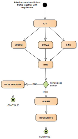
Figure 1.
UML diagram of solution.
When malicious traffic gets to IDS, time frames that can be processed are firstly made, in this case the time frame of one second has been used, during that time we need to count all packages that are received. After we create a time frame and count all packages, three selected algorithms, CUSUM, EWMA, and k-NN need to be applied to get 3 values that indicate if traffic is malicious or not, and those 3 values are combined into TMR with the final result.
There are few scenarios in this case when there are 3 different limit values, and that is where the TMR is going to be used, to determine whether to trigger the alarm or not. These scenarios are shown in Table 1. The large part in determination is the use of three different algorithms for those variable values so the pattern of the DDoS attack can be predicted more easily.
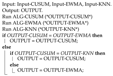
An advantage to TMR is that it has its own backup system, thus if one of those limit’s failed to detect malicious traffic, the other two will do the job. As shown in Algorithm 1, the output values of three algorithms CUSUM, EWMA, and k-NN are compared for the two same values. Possible output results are 0 and 1 which indicates whether an attack is happening or not. First, CUSUM and EWMA are compared, if those two values are the same then the output will be the same as CUSUM. If they are different, a second comparison is made between CUSUM and k-NN, which will give a final result. If k-NN equals to CUSUM than we are taking the CUSUM value as result and if not we are taking EWMA or k-NN value as a result because that means that EWMA and k-NN have the same values which is the opposite from the CUSUM value and that is the case we need. With that we can decide whether to trigger the alarm or not. Conclusion is what the majority decides.
| Algorithm 1: Application of triple modular redundancy for attack triggering in one IDS |
 |
4.2. Implementation
This solution is written in Python language because of its easy-to-use architecture and various options of network manipulation and a large number of alarming libraries.
Firstly, algorithms with training dataset [35] are run so at the end we can get final evaluation results with the CIC-DDoS2019 dataset [36]. Python contains many possibilities, with a few libraries that can be chosen to work with such as [44] where both EWMA and CUSUM algorithms are already implemented and ready to use, and for a k-NN algorithm there is also few out of the box solutions that can be used and one of them is [45].
Traffic Modeling
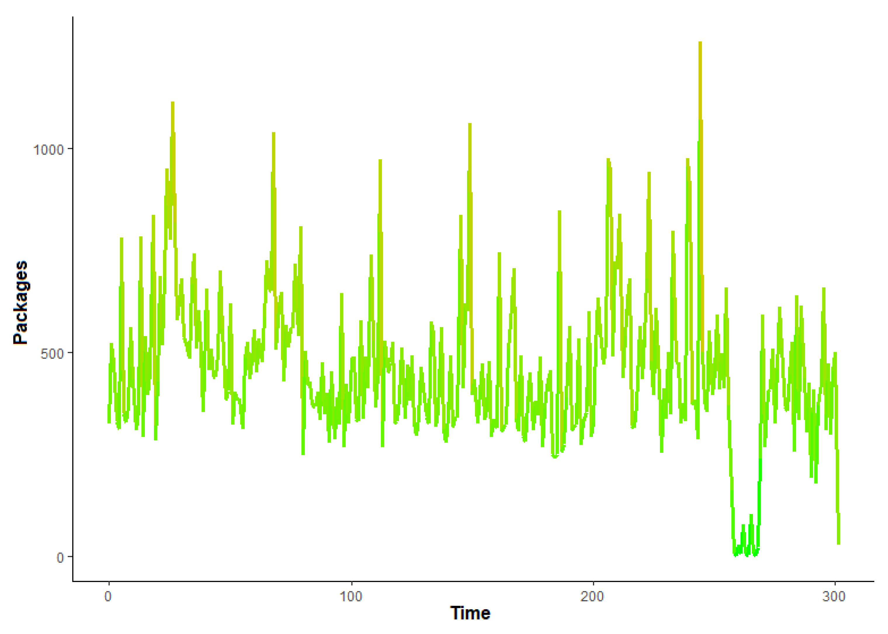
Figure 2 represents chart of legitimate traffic, where the number of received packages during the period of time is shown. The time series in this case is 1 s, there is nothing unusual about this traffic, and the number of packages is almost constantly between 300 and 700 with some minor deflections. While Figure 3 represents chart of illegitimate traffic with large deflections in the number of received packages, at peak the number of packages is 20,000 per second.
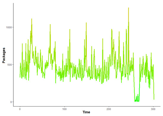
Figure 2.
Legitimate traffic variations in time.
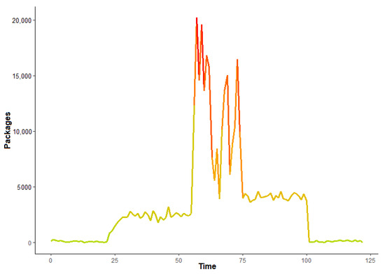
Figure 3.
Illegitimate traffic variations in time.
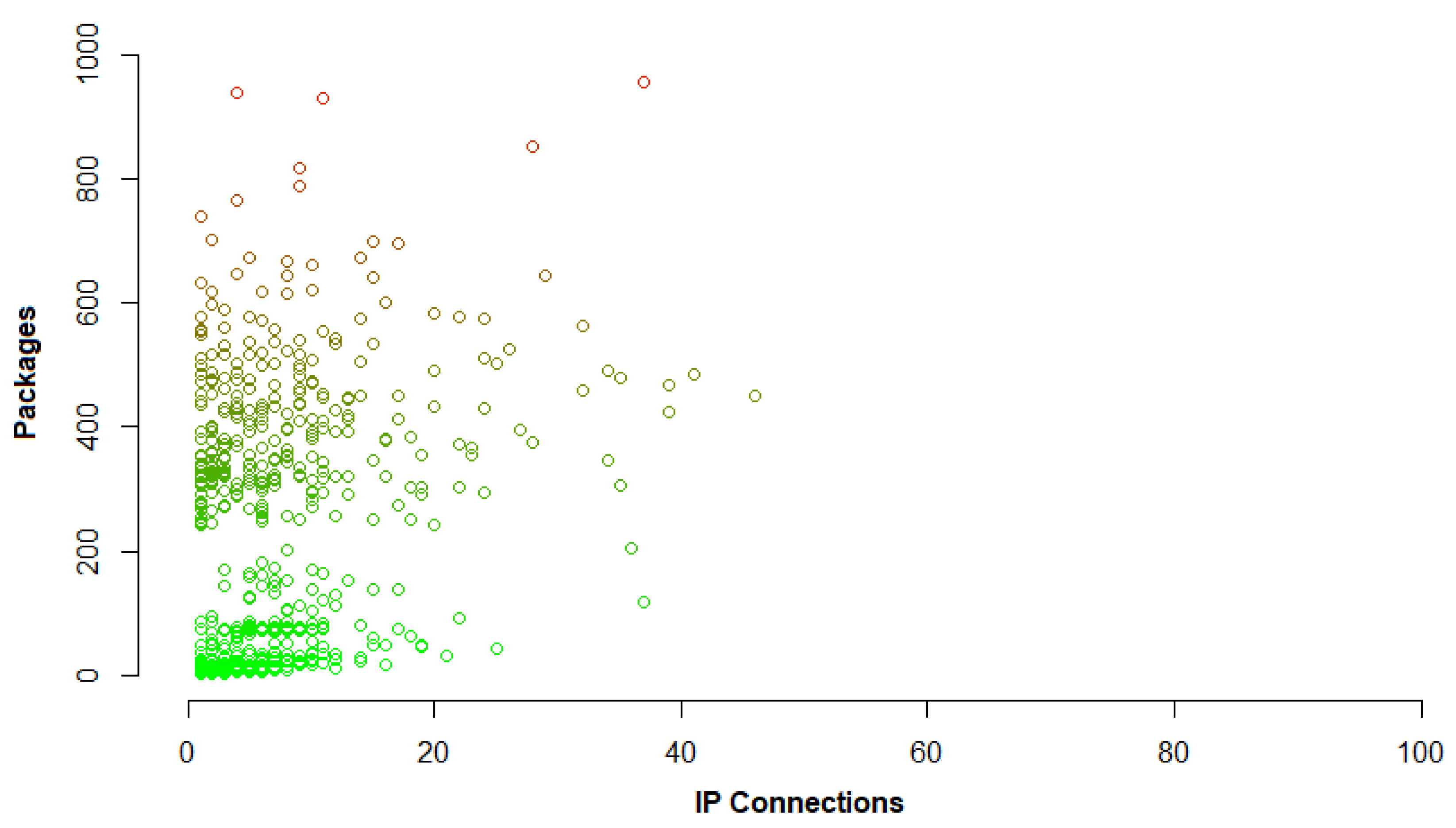
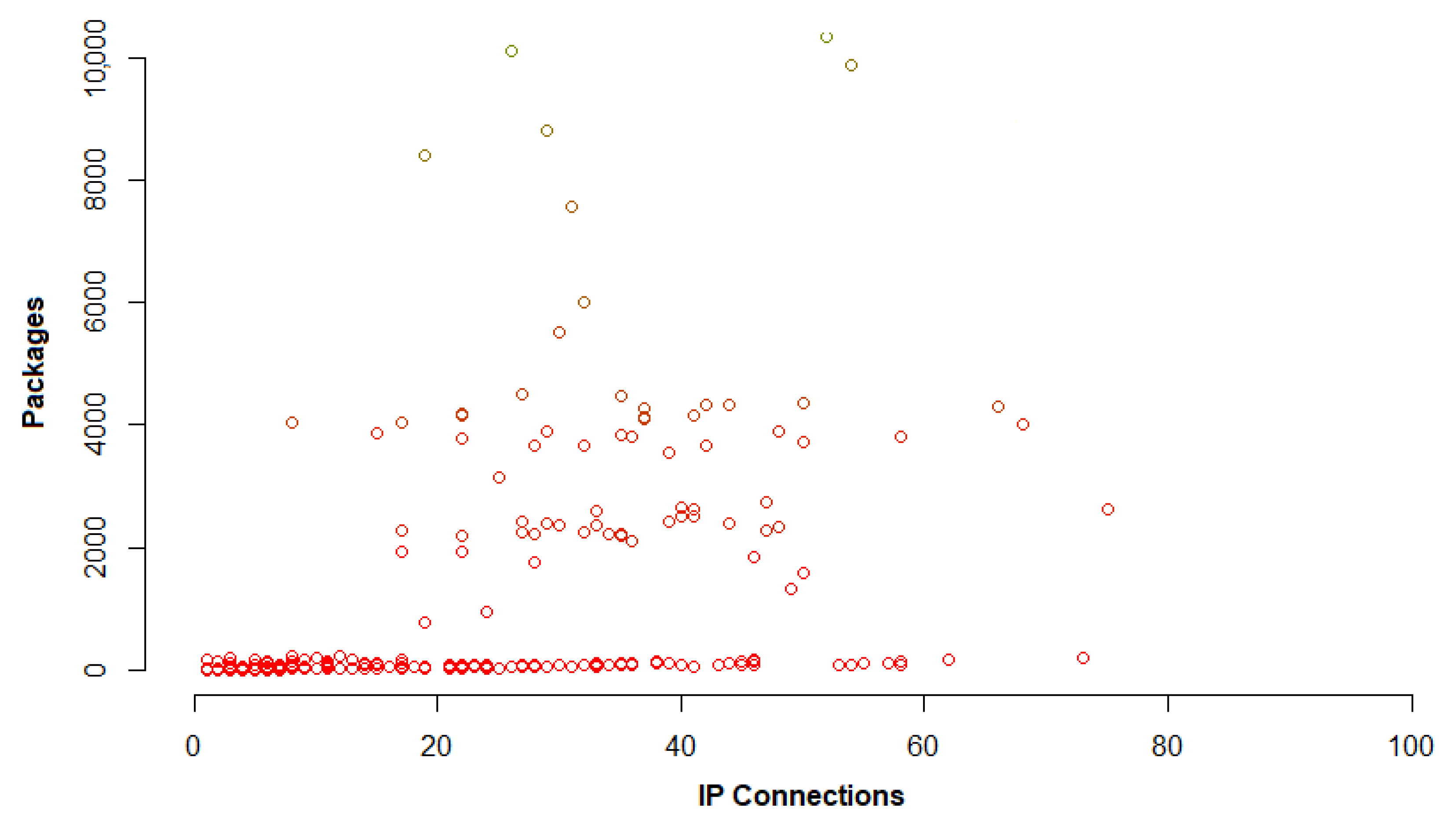
When it comes to traffic coherence we need to look deeper into traffic connections, all Internet Protocol (IP) connections need to be counted as described before [14]. That means when the time interval T is chosen, in this case that is 1 s, during that interval all IP connections or to be a more precise number of packages exchanged between two IP addresses need to be counted. After that, noticing irregularity in the graphic representations is the next step. Figure 4 represents legitimate traffic again, the same one that was represented in Figure 2 and there is shown pretty consistent number of packages per number of IP connections. Figure 5 represents illegitimate traffic where there is no coherence between packages over IP connections, in this case illegitimate traffic is separated from legitimate.
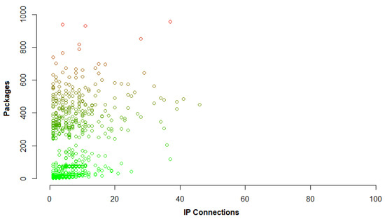
Figure 4.
Number of packages vs number of Internet Protocol (IP) connections for legitimate traffic.

Figure 5.
Number of packages vs number of IP connections for illegitimate traffic.
4.3. Obtained Results
The three algorithms are tested to see all the advantages of the presented solution. First marking the data is being done, so these algorithms can be compared to some benchmark values. Marked data that have 1059 time series, each in duration of one second, are represented at Figure 6, where network traffic is given in the number of packages and the time is given in seconds.

Figure 6.
Marked User Datagram Protocol (UDP) flooding attack traffic.
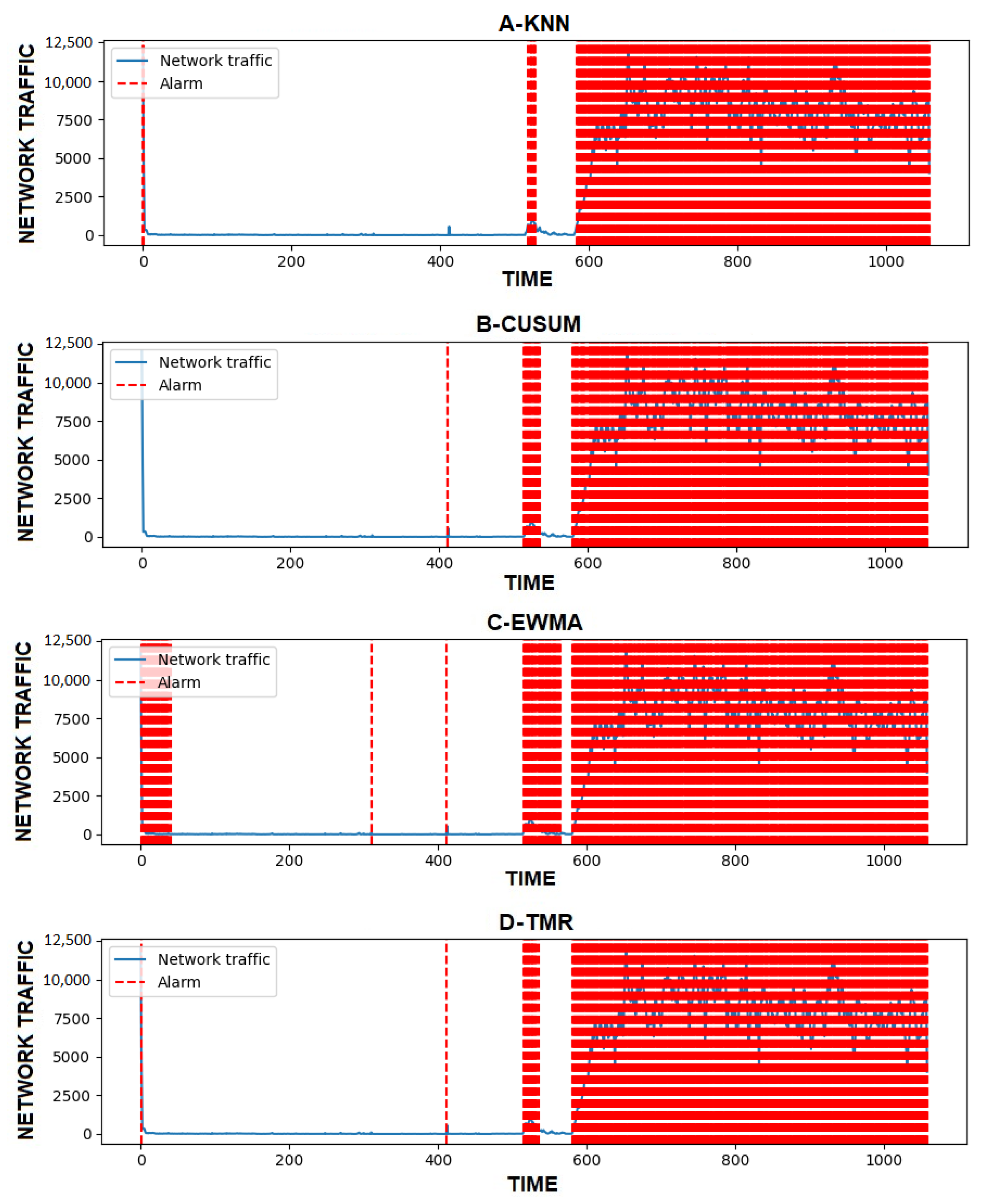
After marking the malicious traffic, we started measuring precision, accuracy, recall, and F1 for three selected algorithms CUSUM, EWMA, and k-NN algorithm to see how they perform and compare. In the end they are combined using TMR to get the best possible result. In Figure 7A, the k-NN algorithm represents how the k-nearest neighbors algorithm detects malicious UDP flooding attack traffic, in Figure 7B, the CUSUM shows the same thing but for CUSUM, and finally Figure 7C shows EWMA. In Figure 7D, TMR is represented using TMR applied using these three algorithms.
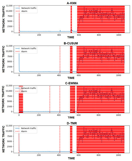
Figure 7.
UDP flooding attack detection.
After this IDS software solution is finished and well tested, Table 3 represents a comparison between the cases when only one limit has been used, and when three limits are used, all three algorithms CUSUM, EWMA, and k-NN are combined together in TMR. Advantages are that accuracy, precision, and F1 are all higher with the usage of TMR than any of other three algorithms separately, and in case of recall almost identical to the best result. In Table 3, values that are presented are between 0 and 1 and they represent the percentage divided by 100.

Table 3.
UDP flooding attack evaluation results.
As shown we can conclude that the proposed methodology gives better precision and a F1 rate in comparison to any of these algorithms individually.
5. Discussion
In addition to our results from Table 3, we have conducted a cross validation on the CIC-DDoS2019 dataset to confirm our results, and that is shown in Table 4 where TMR showed better precision and accuracy than all three algorithms separately, and is second best for F1 and recall results. These results are better than any of these algorithms individually. To perform cross validation, the dataset was sectioned in six even parts, and with that we performed our evaluation for each set individually. In the end we got a similar results to what was achieved during the first evaluation.

Table 4.
UDP flooding attack in cross validation results.
The downside to this approach is that the time with TMR is longer than using any of these three algorithms individually. That is because of the comparison between them, but it is not significantly longer because only three algorithms have been used. Regarding this, the proposed methodology can be used in real-time systems with small adjustments, it would certainly have some delay but the precision would be higher.
With TMR, the balance between these algorithms is achieved because CUSUM is not triggering if the number of packages starts dropping down during an attack, and with the EWMA problem, if the attack lasts for a longer period without oscillations in the number of packages, then EWMA recognizes that as a regular traffic. The k-NN algorithm is the best of these three but also not good enough to beat TMR. With these three algorithms used for TMR, we managed to get most out of them because not every increasing in number of packages is an attack, and also not every drop in number of packages is the end of an attack. The limitation of the discussed solution is next, if there is a sudden drop in number of packages in ongoing attack it will detect that the attack has stopped which is not the case. To overcome this problem we need to tune these algorithms more using other datasets with different attack scenarios.
Comparing our results to other solutions that are using the CIC-DDoS2019 dataset such as [46,47], we can see that our results are among higher values with a percentage over 90 and in some cases even higher. But comparing our results with some other research results is not valid in our case, because we have shown here if we have any three algorithms, whether they are giving better or worse results, we are going to get better results than each of them individually. For example if we have selected three algorithms where all three have good accuracy and precision, like for example we saw in the case of k-NN here, we would have very high results combining them into TMR, but if we select three algorithms with low percentage values, we would get improvement with the application of TMR but that cannot differ much than the selected algorithms.
All results can be replicated by using scripts from [48], also these scripts can be used for further data evaluation and upgrading of the existing solution.
6. Conclusions
In this paper, a new detection limit determination approach using triple modular redundancy was proposed for IDS in order to detect and after that to prevent DDoS attacks. Nowadays, 24/7 protection as well as the alarming feature is necessary for IDS. In this solution where three algorithms are combined to get the best possible result as presented in Table 3, by using TMR the best accuracy and F1 were achieved, and recall with precision was very high when comparing each of these three algorithms separately with the final TMR result. In Table 4, precision and accuracy were the best while F1 and recall had high values, showing again that our approach was correct and gave better results. Using TMR we should get an improvement in results with any three existing algorithms comparing them to themselves. Also instead of triple modular redundancy we can use n-modular redundancy where n is an odd number.
It is important to remark what is most important that enables proposed methodology.
- New things:
- Using redundancy to get better results by including existing algorithms;
- Combining EWMA, CUSUM, and k-nearest neighbours algorithm together in one TMR;
- Using one dataset for training and other to make evaluation and to make it more comparable.
- Advantages:
- Higher accuracy than each included method individually;
- Easy for implementation using Python.
The downside of proposed solution is the time of execution for TMR, as it uses three algorithms that need to be calculated first. In the best case scenario, TMR would be fast as the slowest of these three algorithms, and with modern multi-threading systems that is probably the most usual case so it is not a big loss in performances if better results are taken into account. This solution also can be used in real-time systems with certain performance limitations and combined with other software solutions that can be part of intrusion prevention systems. That is the reason why triple modular redundancy is selected and not the N-modular redundancy, the gain in results cannot be much bigger than with TMR but time of execution would be higher. The authors plan to deal with the choice of the type and number of existing algorithms for determining an attack in one in the general case N-redundant optimization of that procedure. In addition, the subject of the author’s interest in future work will be the inclusion and application of different types of algorithms i.e., approaches in the mentioned N-redundant optimization of this proposed procedure, tests with newer datasets will be conducted with different types of algorithms for better optimization, and an even better result. Large scale attacks would also be discussed and tried out, together with different alarming options for easier implementation into Intrusion Prevention Systems.
Author Contributions
Formal analysis, M.R.; Writing—review and editing, D.R. and M.R.; Investigation, data curation, I.B.; Software, I.B. and A.M.; Validation, writing—original draft preparation I.B. and V.N.; Resources, visualization, I.B. and M.Č.; project administration, funding acquisition, A.Đ. All authors have read and agreed to the published version of the manuscript.
Funding
This paper is supported by Science technology park Niš.
Institutional Review Board Statement
Not applicable.
Informed Consent Statement
Not applicable.
Data Availability Statement
The following materials are available online at https://ieee-dataport.org/open-access/iot-network-intrusion-dataset (accessed on 15 November 2020) and CIC-DDoS2019 dataset at https://www.unb.ca/cic/datasets/ddos-2019.html (accessed on 15 January 2021). We have used UDP recorded traffic of the attack from these datasets, and benign traffic for comparison.
Conflicts of Interest
The authors declare no conflict of interest.
Abbreviations
The following abbreviations are used in this manuscript:
| IDS | Intrusion Detection System |
| IPS | Intrusion Prevention System |
| DDoS | Distributed Denial of Service |
| TMR | Triple Modular Redundancy |
| CUSUM | Cumulative Sum |
| EWMA | Exponentially Weighted Moving Average |
| k-NN | k-Nearest Neighbors |
| UDP | User Datagram Protocol |
| HTTP | Hypertext Transfer Protocol |
| CERT | Computer emergency response team |
| TP | True Positive |
| TN | True Negative |
| FP | False Positive |
| FN | False Negative |
References
- Pu, S. Choosing parameters for detecting DDoS attack. In Proceedings of the 2012 International Conference on Wavelet Active Media Technology and Information Processing (ICWAMTIP), Chengdu, China, 17–19 December 2012; pp. 239–242. [Google Scholar] [CrossRef]
- Lee, K.; Kim, J.; Kwon, K.H.; Han, Y.; Kim, S. DDoS attack detection method using cluster analysis. Expert Syst. Appl. 2008, 34, 1659–1665. [Google Scholar] [CrossRef]
- DDoS Attack Types and Mitigation Methods. Available online: https://www.imperva.com/learn/ddos/ddos-attacks (accessed on 12 December 2020).
- Sanmorino, A.; Yazid, S. DDoS attack detection method and mitigation using pattern of the flow. In Proceedings of the 2013 International Conference of Information and Communication Technology (ICoICT), Bandung, Indonesia, 20–22 March 2013; pp. 12–16. [Google Scholar] [CrossRef]
- Khraisat, A.; Gondal, I.; Vamplew, P. Survey of intrusion detection systems: Techniques, datasets and challenges. Cybersecurity 2019, 2, 1–22. [Google Scholar] [CrossRef]
- Zhang, Z.; Liu, D.; Wei, Z.; Sun, C. Research on Triple Modular Redundancy Dynamic Fault-Tolerant System Model. In Proceedings of the First International Multi-Symposiums on Computer and Computational Sciences (IMSCCS’06), Hanzhou, China, 20–24 June 2006; pp. 572–576. [Google Scholar] [CrossRef]
- Lyons, R.E.; Vanderkulk, W. The use of triple-modular redundancy to improve computer reliability. IBM J. Res. Dev. 1962, 6, 200–209. [Google Scholar] [CrossRef]
- Abraham, J.A.; Siewiorek, D.P. An algorithm for the accurate reliability evaluation of triple modular redundancy networks. IEEE Trans. Comput. 1974, 100, 682–692. [Google Scholar] [CrossRef]
- Shanbhag, S.; Wolf, T. Accurate anomaly detection through parallelism. IEEE Netw. 2009, 23, 22–28. [Google Scholar] [CrossRef]
- Machaka, P.; Bagula, A.; Nelwamondo, F. Using exponentially weighted moving average algorithm to defend against DDoS attacks. In Proceedings of the 2016 Pattern Recognition Association of South Africa and Robotics and Mechatronics International Conference (PRASA-RobMech), Stellenbosch, South Africa, 30 November–2 December 2016; pp. 1–6. [Google Scholar] [CrossRef]
- Wang, H.; Zhang, D.; Shin, K.G. Change-point monitoring for the detection of DoS attacks. Trans. Dependable Secur. Comput. 2004, 1, 193–208. [Google Scholar] [CrossRef]
- Özçelik, I.; Brooks, R.R. Cusum-entropy: An efficient method for DDoS attack detection. In Proceedings of the 2016 4th International Istanbul Smart Grid Congress and Fair (ICSG), Istanbul, Turkey, 20–21 April 2016; pp. 1–5. [Google Scholar] [CrossRef]
- Santosh, K.M.; Isaac, E. Defending DDoS Attack using Stochastic Model based Puzzle Controller. IJCSNS Int. J. Comput. Sci. Netw. Secur. 2013, 13, 100–105. [Google Scholar]
- Rahmani, H.; Sahli, N.; Kamoun, F. A Traffic Coherence Analysis Model for DDoS Attack Detection. In Proceedings of the International Conference on Security and Cryptography, Milan, Italy, 7–10 July 2009; pp. 148–154. [Google Scholar]
- Douligeris, C.; Mitrokotsa, A. DDOS Attacks and Defense Mechanisms: A classification. In Proceedings of the I3rd IEEE International Symposium on Signal Processing and Information Technology, Darmstadt, Germany, 17 December 2003; pp. 190–193. [Google Scholar] [CrossRef]
- Mahjabin, T.; Xiao, Y.; Sun, G.; Jiang, W. A survey of distributed denial-of-service attack, prevention, and mitigation techniques. Int. J. Distrib. Sens. Netw. 2017, 13, 1550147717741463. [Google Scholar] [CrossRef]
- David, J.; Thomas, C. DDoS Attack Detection Using Fast Entropy Approach on Flow- Based Network Traffic. In Proceedings of the 2nd International Symposium on Big Data and Cloud Computing Challenges, VIT University, Chennai, India, 12–13 March 2015; pp. 30–36. [Google Scholar] [CrossRef]
- Wang, Y. A Hybrid Intrusion Detection System. Ph.D. Thesis, Iowa State University, Ames, IA, USA, 2004. [Google Scholar]
- Smaha, S.E. Haystack: An intrusion detection system. In Proceedings of the Fourth Aerospace Computer Security Applications, Orlando, FL, USA, 12–16 September 1988; pp. 37–44. [Google Scholar] [CrossRef]
- Yusof, A.R.; Udzir, N.I.; Selamat, A.; Hamdan, H.; Abdullah, M.T. Adaptive feature selection for denial of services (DoS) attack. In Proceedings of the 2017 IEEE Conference on Application, Information and Network Security (AINS), Miri, Malaysia, 13–14 November 2017; pp. 81–84. [Google Scholar] [CrossRef]
- Kim, J.; Kim, J.; Kim, H.; Shim, M.; Choi, E. CNN-Based Network Intrusion Detection against Denial-of-Service Attacks. Electronics 2020, 9, 916. [Google Scholar] [CrossRef]
- Mahfouz, A.; Abuhussein, A.; Venugopal, D.; Shiva, S. Ensemble Classifiers for Network Intrusion Detection Using a Novel Network Attack Dataset. Future Internet 2020, 12, 180. [Google Scholar] [CrossRef]
- Faizal, M.A.; Zaki, M.M.; Shahrin, S.; Robiah, Y.; Rahayu, S.S.; Nazrulazhar, B. Threshold Verification Technique for Network Intrusion Detection System. arXiv 2009, arXiv:0906.3843. [Google Scholar]
- Idika, N.; Mathur, A. Survey of Malware Detection Techniques; Purdue University: West Lafayette, Indiana, 2007. [Google Scholar]
- Patel, D.; Srinivasan, K.; Chang, C.-Y.; Gupta, T.; Kataria, A. Network Anomaly Detection inside Consumer Networks—A Hybrid Approach. Electronics 2020, 9, 923. [Google Scholar] [CrossRef]
- Ahsan, M.; Mashuri, M.; Kuswanto, H.; Prastyo, D.D. Intrusion Detection System using Multivariate Control Chart Hotelling’s T2 based on PCA. Int. J. Adv. Sci. Eng. Inf. Technol. 2018, 8, 1905–1911. [Google Scholar] [CrossRef]
- Silva, L.A.; Leithardt, V.R.Q.; Rolim, C.O.; González, G.V.; Geyer, C.F.R.; Silva, J.S. PRISER: Managing Notification in Multiples Devices with Data Privacy Support. Sensors 2019, 19, 3098. [Google Scholar] [CrossRef]
- Sales Mendes, A.; Jiménez-Bravo, D.M.; Navarro-Cáceres, M.; Reis Quietinho Leithardt, V.; Villarrubia González, G. Multi-Agent Approach Using LoRaWAN Devices: An Airport Case Study. Electronics 2020, 9, 1430. [Google Scholar] [CrossRef]
- Haider, S. A Deep CNN Ensemble Framework for Efficient DDoS Attack Detection in Software Defined Networks. IEEE Access 2020, 8, 53972–53983. [Google Scholar] [CrossRef]
- Gupta, B.B.; Dahiya, A. Distributed Denial of Service (DDoS) Attacks: Classification, Attacks, Challenges and Countermeasures, 1st ed.; CRC Press: Boca Raton, FL, USA, 2021. [Google Scholar] [CrossRef]
- Sklavounos, D.; Edoh, A.; Plytas, M. A Statistical Approach Based on EWMA and CUSUM Control Charts for R2L Intrusion Detection. In Proceedings of the 2017 Cybersecurity and Cyberforensics Conference (CCC), London, UK, 21–23 November 2017; pp. 25–30. [Google Scholar] [CrossRef]
- Leu, F.Y.; Yang, W.J. Intrusion Detection with CUSUM for TCP-Based DDoS. In Proceedings of the Embedded and Ubiquitous Computing—EUC 2005 Workshops, Nagasaki, Japan, 6–9 December 2005; pp. 1255–1264. [Google Scholar]
- Zhang, T. Cumulative sum algorithm for detecting SYN flooding attacks. arXiv 2012, arXiv:1212.5129. [Google Scholar]
- Vu, N.H.; Choi, Y.; Choi, M. DDoS attack detection using K-Nearest Neighbor classifier method. In Proceedings of the IASTED International Conference on Telehealth/Assistive Technologies, Baltimore, MD, USA, 16–18 April 2008; pp. 248–253. [Google Scholar]
- IoT Network Intrusion Dataset. Available online: https://ieee-dataport.org/open-access/iot-network-intrusion-dataset (accessed on 15 November 2020).
- Sharafaldin, I.; Lashkari, A.H.; Hakak, S.; Ghorbani, A.A. Developing Realistic Distributed Denial of Service (DDoS) Attack Dataset and Taxonomy. In Proceedings of the IEEE 53rd International Carnahan Conference on Security Technology, Chennai, India, 1–3 October 2019; Available online: https://www.unb.ca/cic/datasets/ddos-2019.html (accessed on 15 January 2021). [CrossRef]
- Liu, W.; Ren, P.; Liu, K.; Duan, H. Behavior-based malware analysis and detection. In Proceedings of the 2011 First International Workshop on Complexity and Data Mining, Nanjing, Jiangsu, China, 24–28 September 2011; pp. 39–42. [Google Scholar] [CrossRef]
- Zhou, Y.; Li, J. Research of network traffic anomaly detection model based on multilevel auto-regression. In Proceedings of the 2019 IEEE 7th International Conference on Computer Science and Network Technology (ICCSNT), Dalian, China, 19–20 October 2019; pp. 380–384. [Google Scholar] [CrossRef]
- Shernta, S.; Tamtum, A. Using triple modular redundant (tmr) technique in critical systems operation. Int. J. Comput. Sci. Netw. Secur. 2013, 13, 100–105. [Google Scholar] [CrossRef]
- Čabarkapa, M.; Mišić, J.; Ranđelović, D.; Nedeljković, S.; Nikolić, V. An Advanced Quick-Answering System Intended for the e-Government Service in the Republic of Serbia. Acta Polytech. Hung. 2019, 16, 153–174. [Google Scholar]
- Machaka, P.; McDonald, A.; Nelwamondo, F.; Bagula, A. Using the Cumulative Sum Algorithm against Distributed Denial of Service Attacks in Internet of Things. In Proceedings of the International Conference on Context-Aware Systems and Applications, Thu Dau Mot, Vietnam, 24–25 November 2016; pp. 66–72. [Google Scholar]
- Čisar, P.; Čisar, S.; Bošnjak, S.; Marav, S. EWMA algorithm in network practice. Int. J. Comput. 2010, 5, 160–170. [Google Scholar] [CrossRef]
- Atawodi, I. A Machine Learning Approach to Network Intrusion Detection System Using K Nearest Neighbor and Random Forest. Master’s Thesis, The University of Southern Mississippi, Hattiesburg, MS, USA, May 2019. [Google Scholar]
- Python Pandas Library. Available online: https://pandas.pydata.org/pandas-docs/version/0.17.0/generated/pandas.ewma.html (accessed on 15 November 2020).
- Scikit Learn. Available online: https://scikit-learn.org/stable/modules/generated/sklearn.neighbors.KNeighborsClassifier.html (accessed on 7 February 2021).
- Elsayed, M.; Le-Khac, N.A.; Dev, S.; Jurcut, A. DDoSNet: A Deep-Learning Model for Detecting Network Attacks. In Proceedings of the 21st IEEE International Symposium on a World of Wireless, Mobile and Multimedia Networks (IEEE WoWMOM 2020), Cork, Ireland, 31 August–3 September 2020. [Google Scholar] [CrossRef]
- Sales de Lima Filho, F.; Silveira, F.A.F.; Brito Junior, A.M.; Vargas-Solar, G.; Silveira, L.F. Smart Detection: An Online Approach for DoS/DDoS Attack Detection Using Machine Learning. Secur. Commun. Netw. 2019, 2019, 1574749. [Google Scholar] [CrossRef]
- Python and R Scripts for TMR. Available online: https://github.com/miljkomocnik/3ADetection (accessed on 10 February 2021).
Publisher’s Note: MDPI stays neutral with regard to jurisdictional claims in published maps and institutional affiliations. |
© 2021 by the authors. Licensee MDPI, Basel, Switzerland. This article is an open access article distributed under the terms and conditions of the Creative Commons Attribution (CC BY) license (http://creativecommons.org/licenses/by/4.0/).


