Article

The Flexible Burr X-G Family: Properties, Inference, and Applications in Engineering Science

1
Department of Statistics and Operations Research, King Saud University, Riyadh 11362, Saudi Arabia
2
Department of Mathematics and Statistics, College of Science, Imam Mohammad Ibn Saud Islamic University (IMSIU), Riyadh 11432, Saudi Arabia
3
Department of Mathematics, Tafila Technical University, Tafila 66110, Jordan
4
Department of Mathematics, Faculty of Science, Tanta University, Tanta 31527, Egypt
5
Department of Statistics, Mathematics and Insurance, Benha University, Benha 13511, Egypt
*
Author to whom correspondence should be addressed.
Symmetry 2021, 13(3), 474; https://doi.org/10.3390/sym13030474
Submission received: 18 February 2021 / Revised: 5 March 2021 / Accepted: 9 March 2021 / Published: 14 March 2021

Abstract

:
In this paper, we introduce a new flexible generator of continuous distributions called the transmuted Burr X-G (TBX-G) family to extend and increase the flexibility of the Burr X generator. The general statistical properties of the TBX-G family are calculated. One special sub-model, TBX-exponential distribution, is studied in detail. We discuss eight estimation approaches to estimating the TBX-exponential parameters, and numerical simulations are conducted to compare the suggested approaches based on partial and overall ranks. Based on our study, the Anderson–Darling estimators are recommended to estimate the TBX-exponential parameters. Using two skewed real data sets from the engineering sciences, we illustrate the importance and flexibility of the TBX-exponential model compared with other existing competing distributions.

1. Introduction

Recently, several generalized families (also known as generators) of univariate distribution have been constructed based on classical distributions. These generators provide greater flexibility by adding one or more parameters to a baseline model. For example, Marshall-Olkin-G [1], transmuted-G [2], odd Lomax-G [3], Marshall-Olkin alpha-power-G [4], and odd Dagum-G [5], amongst others. The flexibility of these generalized models can be expressed in terms of their ability to model various real-life data encountered in different applied fields, in particular, reliability engineering, medicine, survival analysis, agriculture, actuarial sciences, demography, and others. The flexibility of generalized models is important to model several shapes of aging and failure criteria.
Shaw and Buckley [2] introduced a useful technique of adding a new parameter to an existing distribution called the transmuted-G (T-G) family, which is adopted to propose generalized forms of classical distributions. The T-G family has received widespread recognition in the literature and more than 70 generalized models have been proposed based on the T-G class. For example, the transmuted log-logistic [6], transmuted Marshall-Olkin Fréchet [7], and transmuted Burr XII [8], amongst others. Tahir and Cordeiro [9] listed more than 50 generalized models that were extended using the T-G family.
Several authors have constructed extended forms of the T-G class. Some notable examples are: transmuted exponentiated generalized-G [10], transmuted geometric-G [11], Kumaraswamy transmuted-G [12], generalized transmuted-G [13], and transmuted transmuted-G [14], and complementary generalized transmuted Poisson-G families [15].
The cumulative distribution function (CDF) of the T-G class has the form
F ( x ; ρ , Φ ) = W ( x ; Φ ) 1 + ρ ρ W ( x ; Φ ) , x > 0 , | ρ | 1 .
Its probability density function (PDF) reduces to
f ( x ; ρ , Φ ) = w ( x ; Φ ) 1 + ρ 2 ρ W ( x ; Φ ) , x > 0 , | ρ | 1 ,
where ρ is a shape parameter; W ( x ; Φ ) and w ( x ; Φ ) are the baseline CDF and PDF, respectively; with parameter vector Φ . The T-G density is a mixture of a baseline density and an exponentiated-G (Exp-G) density with power parameter 2. For ρ = 0 , the T-G class reduces to the baseline distribution.
We were motivated to adopt the T-G family to extend another class of distributions called the Burr X-G (BX-G) class [16] and provide a wider family that can be used to effectively model various real-life data. Hence, the aim of this study was two-fold: First, we wanted to propose a new extended form of the BX-G class based on the T-G class, called the transmuted Burr X-G (TBX-G) family. Various general properties of the TBX-G class are derived. Secondly, we discussed eight estimation methods of the TBX-exponential parameters: maximum likelihood (MLE), Anderson–Darling (ADE), right-tail Anderson–Darling (RADE), Cramér–von Mises minimum distance (CVME), ordinary least squares (OLSE), weighted least-squares (WLSE), maximum product of spacings (MPSE), and percentile (PCE) estimators, and compared them, in terms of their absolute value of biases ( B i a s ), mean squared error (MSE), and mean relative error (MRE), using extensive simulations to develop a guideline for choosing the best estimation approach that produces more accurate estimates for the model parameters. The estimation methods were compared based on partial and overall ranks to choose the best estimation method, which will be of important interest to applied statisticians, practitioners, and engineers.
Yousof et al. [16] proposed a new generator for the construction of new extended and flexible versions from classical models, which is known as BX-G. Consider the PDF and CDF of a baseline distribution with a parameter vector Φ , g ( x ; Φ ) , and G ( x ; Φ ) ; then, the CDF of the BX-G class, with a positive-shape parameter φ , takes the form
W B X ( x ; φ , Φ ) = 1 e G ( x ; Φ ) G ¯ ( x ; Φ ) 2 φ , x > 0 , φ > 0 .
The PDF of the BX-G family reduces to
w B X ( x ; φ , Φ ) = 2 φ G ( x ; Φ ) g ( x ; Φ ) 1 G ( x ; Φ ) 3 1 e G ( x ; Φ ) G ¯ ( x ; Φ ) 2 φ 1 e G ( x ; Φ ) G ¯ ( x ; Φ ) 2 , x > 0 , φ > 0 .
To this end, we define the CDF and PDF of the proposed TBX-G family. By inserting Equation (3) into Equation (1), the TBX-G family can be specified by the following CDF (for x > 0 , | ρ | 1 , φ > 0 )
F ( x ; ρ , φ , Φ ) = 1 e G ( x ; Φ ) G ¯ ( x ; Φ ) 2 φ 1 + ρ ρ 1 e G ( x ; Φ ) G ¯ ( x ; Φ ) 2 φ .
The PDF of the TBX-G class has the form
f ( x ; ρ , φ , Φ ) = 2 φ G ( x ; Φ ) g ( x ; Φ ) 1 G ( x ; Φ ) 3 1 e G ( x ; Φ ) G ¯ ( x ; Φ ) 2 φ 1 e G ( x ; Φ ) G ¯ ( x ; Φ ) 2 × 1 + ρ 2 ρ 1 e G ( x ; Φ ) G ¯ ( x ; Φ ) 2 φ .
Hereafter, a random variable ( r v ) with PDF (6) is denoted by X∽TBX-G ( ρ , φ , δ ) . The TBX-G class reduces to the BX-G family with ρ = 0 . The TBX-G is a wider family of continuous distributions. It includes the BX-G family and provides greater flexibility in modeling real life data.
Finally, we summarize the findings of the proposed TBX-G class as follows: (1) Its sub-models provide unimodal, symmetrical, left-skewed, right-skewed, and reversed-J densities. They have decreasing, increasing, bathtub, upside-down bathtub, J-shaped, and reversed-J shaped hazard rates, which are frequently encountered in real-life applied areas. (2) Its special sub-models perform very well compared with other competing models, which are generated by well-known families under the same baseline model. (3) The sub-models generated by the TBX-G class are capable of modeling different shapes of ageing and failure criteria. Hence, the TBX-G can be a useful alternative to several classes for modeling skewed data in application(s).
The reminder of the paper is organized as follows: Two sub-models called the TBX-exponential (TBXE) and TBX-log-logistic (TBXLL) distributions are presented in Section 2. Various general properties of the TBX-G family are explored in Section 3. Properties of the TBXE model are discussed in Section 4. The maximum likelihood estimation for the TBX-G parameters are derived in Section 5. In Section 6, we estimate the TBXE parameters using eight estimation approaches. Section 7 is devoted to studying the behavior of these estimators via simulation results. In Section 8, we illustrate the flexibility of the new class using two real-life applications, showing that the TBXE model can provide a better fit than other competing models. Some concluding remarks are provided in Section 9.

2. Two Sub-Models

In this subsection, we introduce two special models of the TBX-G family based on the exponential and log-logistic models to generate the TBXE and TBXLL distributions, which can provide unimodal, symmetrical, left-skewed, right-skewed, and reversed-J-shaped densities; and decreasing, increasing, bathtub, upside-down bathtub, J-shaped, and reversed-J shaped hazard rates (Figure 1 and Figure 2).

2.1. The TBXE Distribution

Consider the exponential model with PDF, g ( x ; β ) = β e β x , β , x > 0 ; hence, CDF, PDF, and the hazard rate function (HRF) of TBXE are, respectively, given (for β , φ > 0 , and | ρ | 1 ) by
F ( x ; Θ ) = 1 e e β x 1 2 φ 1 + ρ ρ 1 e e β x 1 2 φ , f ( x ; Θ ) = 2 β φ e β x ( e β x 1 ) e e β x 1 2 1 e e β x 1 2 φ 1 × 1 + ρ 2 ρ 1 e e β x 1 2 φ , x > 0
and
h ( x ; Θ ) = 2 β φ e β x ( e β x 1 ) e e β x 1 2 1 e e β x 1 2 φ 1 1 + ρ 2 ρ 1 e e β x 1 2 φ 1 1 e e β x 1 2 φ 1 + ρ ρ 1 e e β x 1 2 φ ,
where Θ = ( β , φ , ρ ) .
Figure 1 illustrates some possible shapes of the PDF and HRF of the TBXE distribution for several selected values of β , φ , and ρ .

2.2. The TBXLL Distribution

Using the PDF and CDF of the log-logistic distribution, g ( x ) = α β α x α 1 x β α + 1 2 , α , β > 0 , x > 0 and G ( x ) = 1 x β α + 1 1 ; hence, the CDF, PDF, and the HRF of TBXLL are, respectively, given (for α , β , φ > 0 , and | ρ | 1 ) by
F ( x ; Θ ) = 1 e x β 2 α φ 1 + ρ ρ 1 e x β 2 α φ , f ( x ; Θ ) = 2 φ α x x β 2 α e x β 2 α 1 e x β 2 α φ 1 1 + ρ 2 ρ 1 e x β 2 α φ , x > 0
and
h ( x ; Θ ) = 2 φ α x x β 2 α e x β 2 α 1 e x β 2 α φ 1 1 + ρ 2 ρ 1 e x β 2 α φ 1 1 e x β 2 α φ 1 + ρ ρ 1 e x β 2 α φ , x > 0 ,
where Θ = ( α , β , φ , ρ ) .
Figure 2 illustrates some possible shapes of the PDF and HRF of the TBXLL distribution for several selected values of α , β , φ , and ρ .

3. Properties of the TBX-G Class

This section deals with the general properties of the TBX-G family, such as expansion for the TBX-G density, quantile function, moments, residual and reversed residual life functions, and order statistics.

3.1. Useful Expansion for the TBX-G Density

Some mathematical properties of the TBX-G family can be confirmed through an algebraic expansion in terms of exponential-G (Exp-G) distribution, which is more efficient than directly computing those by numerical integration of its PDF. The TBX-G PDF can be reformulated as
f ( x ; ρ , φ , Φ ) = 2 ( 1 + ρ ) φ G ( x ; Φ ) g ( x ; Φ ) 1 G ( x ; Φ ) 3 e G ( x ; Φ ) G ¯ ( x ; Φ ) 2 1 e G ( x ; Φ ) 1 G ( x ; Φ ) 2 φ 1 4 ρ φ G ( x ; Φ ) g ( x ; Φ ) 1 G ( x ; Φ ) 3 e G ( x ; Φ ) G ¯ ( x ; Φ ) 2 1 e G ( x ; Φ ) 1 G ( x ; Φ ) 2 2 φ 1 .
For a positive real non-integer, the binomial series holds
( 1 s ) φ 1 = j = 0 ( 1 ) j φ 1 j s j , φ > 0 , s < 1 .
Applying the binomial series in (8) to (7), the TBX-G PDF reduces to
f ( x ; ρ , φ , Φ ) = 2 ( 1 + ρ ) φ G ( x ; Φ ) g ( x ; Φ ) 1 G ( x ; Φ ) 3 i = 0 ( 1 ) i φ 1 i e ( i + 1 ) G ( x ; Φ ) 1 G ( x ; Φ ) 2 4 φ ρ G ( x ; Φ ) g ( x ; Φ ) 1 G ( x ; Φ ) 3 i = 0 ( 1 ) i 2 φ 1 i e ( i + 1 ) G ( x ; Φ ) 1 G ( x ; Φ ) 2 .
Applying the exponential series to the PDF (9), we write
e ( i + 1 ) G ( x ; Φ ) 1 G ( x ; Φ ) 2 = j = 0 ( 1 ) j ( i + 1 ) j j ! G ( x ; Φ ) 2 j 1 G ( x ; Φ ) 2 j .
Combining Equations (9) and (10), the PDF of the TBX-G family follows as
f ( x ; ρ , φ , Φ ) = g ( x ; Φ ) i , j = 0 2 φ ( 1 + ρ ) ( 1 ) i + j ( i + 1 ) j φ 1 i j ! G ( x ; Φ ) 2 j + 1 1 G ( x ; Φ ) 2 j + 3 g ( x ; Φ ) i , j = 0 4 φ ρ ( 1 ) i + j ( i + 1 ) j 2 φ 1 i j ! G ( x ; Φ ) 2 j + 1 1 G ( x ; Φ ) 2 j + 3 .
Using the general binomial expansion in (10) (for ( φ ) m = φ ( φ + 1 ) ( φ + m 1 ) )
( 1 s ) φ = m = 0 ( φ ) m m ! s m , s < 1 ,
where ( φ ) m is the ascending factorial, the TBX-G PDF can be formulated as a linear combination of Exp-G PDFs
f ( x ; ρ , φ , Φ ) = j , k = 0 ξ j , k π ( 2 ( j + 1 ) + k ) ( x ) ,
where π ν ( x ) = ν g ( x ; Φ ) G ( x ; δ ) ν 1 denotes the Exp-G PDF with power parameter ν and
ξ j , k = i = 0 2 φ ( 1 ) i + j ( i + 1 ) j ( 2 j + 3 ) k j ! k ! ( 2 ( j + 1 ) + k ) ( 1 + ρ ) φ 1 i 2 ρ 2 φ 1 i .
Equation (13) of the TBX-G PDF can be used to derive some mathematical properties of the TBX-G family directly from those of Exp-G distribution.

3.2. Quantile Function

The TBX-G quantile function (QF) takes the form
F 1 ( u ) = Q G ( u ) = G 1 log 1 A ρ , φ , u 1 2 1 + log 1 A ρ , φ , u 1 2 , 0 < u < 1 ,
where
A ρ , φ , u = ( ρ + 1 ) + ( ρ + 1 ) 4 ρ u 2 ρ 1 φ
and u is a uniform random variable.

3.3. Moments

Let r . v . Z ( 2 ( j + 1 ) + k ) have an Exp-G PDF, π ( 2 ( j + 1 ) + k ) , with power parameter 2 ( j + 1 ) + k . The rth moment of TBX-G family is obtained from (13) as
μ r = E ( X r ) = j , k = 0 ξ j , k E ( Z ( 2 ( j + 1 ) + k ) r ) .
The moment-generating function (MGF) of the TBX-G family can be calculated from (13) as
M X ( t ) = E ( e t X ) = j , k = 0 ξ j , k M ( 2 ( j + 1 ) + k ) ( t ) ,
where M ( 2 ( j + 1 ) + k ) ( t ) is the MGF of the r v Z ( 2 ( j + 1 ) + k ) .
The sth incomplete moments for the TBX-G class are
φ s ( t ) = t x s f ( x ) d x = j , k = 0 ξ j , k t x s π ( 2 ( j + 1 ) + k ) ( x ) d x ,
where the above integral denotes the sth incomplete moment of the r v Z ( 2 ( j + 1 ) + k ) .
Now, we determine two formulae for the TBX-G first incomplete moment (FIM), which follows from (16) with s = 1 . The first formula of FIM reduces to
φ 1 ( t ) = j , k = 0 ξ j , k I ( 2 ( j + 1 ) + k ) ( t ) ,
where
I ( 2 ( j + 1 ) + k ) ( t ) = t x π ( 2 ( j + 1 ) + k ) ( x ) d x ,
is the FIM of Z ( 2 ( j + 1 ) + k ) . The second formula of the TBX-G FIM is
φ 1 ( t ) = j , k = 0 ξ j , k Λ ( 2 ( j + 1 ) + k ) ( t ) ,
where
Λ ( 2 ( j + 1 ) + k ) ( t ) = ( 2 ( j + 1 ) + k ) 0 G ( t ) Q G ( u ) u 2 j + k + 1 d u ,
can be calculated numerically.

3.4. Residual and Reversed Residual Life Functions

The rth-order moment of the residual life has the following formula
μ r ( t ) = E ( ( X t ) r X > t ) = 1 F ¯ ( t ) t ( x t ) r f ( x ) d x , r 1 = 1 F ¯ ( t ) j , k = 0 ξ j , k * t x r π ( 2 ( j + 1 ) + k ) ( x ) d x ,
where ξ j , k * = ξ j , k h = 0 r r h ( t ) r h . The mean remaining life (life expectancy at age t) of the TBX-G family follows from last formula with r = 1 .
The rth-order moment of reversed residual life has the formula
m r ( t ) = E ( ( t X ) r X t ) = 1 F ( t ) 0 t ( t x ) r f ( x ) d x , r 1 = 1 F ( t ) j , k = 0 ξ j , k * 0 t x r π ( 2 ( j + 1 ) + k ) ( x ) d x .
The mean past lifetime refers to the waiting time that elapses since an item fails, on the condition that the failure occurred in ( 0 , t ) . The mean inactivity time of the TBX-G class is obtained from the above formula with r = 1 .

3.5. Order Statistics

The ordered statistics of a random sample from the TBX-G family are denoted by X ( 1 ) , X ( 2 ) , , X ( n ) , and they have some applications in reliability and survival analysis. The PDF of the ith-order statistic is defined by the following formula
f i ; n ( x ) = f ( x ) B ( i , n i + 1 ) j = 0 n i ( 1 ) j n i j F i + j 1 ( x ) ,
where B ( . , . ) refers to the beta function. Using the PDF and CDF of the TBX-G class, we can write
f ( x ) F i + j 1 ( x ) = h , m = 0 ϕ h , m π ( 2 ( m + 1 ) + h ) ( x ) ,
where
ϕ h , m = 2 φ k = 0 i + j 1 d = 0 ( 1 ) d + m ( d + 1 ) m Γ ( 2 m + h + 3 ) m ! h ! ( 2 ( m + 1 ) + h ) Γ ( 2 m + 3 ) i + j 1 k × ( ρ + 1 ) φ ( i + j ) + k 1 d 2 ρ φ ( i + j + 1 ) + k 1 d .
Combining (19) and (20) gives
f i ; n ( x ) = 1 B ( i , n i + 1 ) j = 0 n i ( 1 ) j n i j h , m = 0 ϕ h , m π ( 2 ( m + 1 ) + h ) ( x ) ,
where π ( 2 ( m + 1 ) + h ) ( x ) is the Exp-G density with parameter 2 ( m + 1 ) + h . Then, the PDF of the TBX-G order statistics is a mixture of Exp-G PDFs.
The moments of X i : n reduce to
E ( X i : n s ) = 1 B ( i , n i + 1 ) j = 0 n i ( 1 ) j n i j h , m = 0 ϕ h , m E ( Z ( 2 ( m + 1 ) + h ) s ) .

4. Properties of TBXE Distribution

4.1. Linear Representation

Using Equation (13) and by applying the binomial expansion [ 1 exp ( β x ) ] 2 j + k + 1 , the PDF of TBXE distribution can be rewritten as
f ( x ; β , φ , ρ ) = j , k = 0 [ 2 ( j + 1 ) + k ] ξ j , k β m = 0 ( 1 ) m 2 j + k + 1 m exp [ ( m + 1 ) β x ] ,
which can be expressed as
f ( x ; β , φ , ρ ) = m = 0 ν m g m + 1 ( x ) ,
where
ν m = j , k = 0 ( 1 ) m [ 2 ( j + 1 ) + k ] ξ j , k m + 1 2 j + k + 1 m ,
ξ j , k = i = 0 2 φ ( 1 ) i + j ( i + 1 ) j ( 2 j + 3 ) k j ! k ! ( 2 ( j + 1 ) + k ) ( 1 + ρ ) φ 1 i 2 ρ 2 φ 1 i
and g m + 1 ( x ) = ( m + 1 ) β exp [ ( m + 1 ) β x ] denotes the exponential density with scale parameter ( m + 1 ) β . Then, the TBXE PDF can be expressed as a single linear combination of exponential densities. Let X be a random variable having an exponential distribution with PDF g ( x ) = β exp ( β x ) , x > 0 , β > 0 . Then, the r th ordinary and incomplete moments and the MGF of X are
μ r = β r r ! , ϕ r ( t ) = β r γ ( r + 1 , β t ) , M ( t ) = β β t , t 0 ,
respectively, where γ ( r + 1 , β t ) is the lower incomplete gamma function.

4.2. QF, Moments, and MGF

The QF of the TBXE distribution is given by
Q E ( u ) = 1 β log log 1 1 2 ρ ( ρ + 1 ) ( ρ + 1 ) 2 4 ρ u 1 / ϕ + 1 .
The rth moment of the TBXE distribution follows from Equation (23) as
μ r = r ! m = 0 ν m [ ( m + 1 ) β ] r .
Based on Equation (23), the rth incomplete moment of the TBXE distribution takes the form
ϕ r ( t ) = m = 0 ν m [ ( m + 1 ) β ] r γ ( r + 1 , ( m + 1 ) β t ) .
The FIM of X follows from the last equation as
ϕ 1 ( t ) = m = 0 ν m [ ( m + 1 ) β ] 1 γ ( 2 , ( m + 1 ) β t ) .
The MGF of the TBXE distribution is given by
M ( t ) = m = 0 ν m ( m + 1 ) β ( m + 1 ) β t .

4.3. Mean Residual Life and Mean Inactivity Time

The mean residual life (MRL), or life expectancy at age t, represents the expected additional life length for a unit, which is alive at age t.
The MRL of X is
m ( t ) = 1 ϕ 1 ( t ) S ( t ) t ,
where ϕ 1 ( t ) is given in Equation (27) and S ( t ) is the survival function of the TBXE distribution. Then, we obtain
m ( t ) = 1 S ( t ) 1 m = 0 ν m [ ( m + 1 ) β ] 1 γ ( 2 , ( m + 1 ) β t ) t .
The mean inactivity time (MIT) represents the waiting time elapsed since the failure of an item on the condition that this failure occurred in ( 0 , t ) .
The MIT of TBXE distribution is given by
M I ( t ) = t ϕ 1 ( t ) F ( t ) = t 1 F ( t ) m = 0 ν m [ ( m + 1 ) β ] 1 γ ( 2 , ( m + 1 ) β t ) .

5. Maximum Likelihood Estimation

This section discusses the MLE of the TBX-G parameters. Let x 1 , , x n be a random sample from the TBX-G class with ψ = ( ρ , φ , Φ T ) T being a parameter vector. The log-likelihood for ψ has the form
( ψ ) = n log ( 2 ) + n log ( φ ) + i = 1 n log g ( x i ; Φ ) 3 i = 1 n log G ¯ ( x i ; Φ ) + i = 1 n log G ( x i ; Φ ) i = 1 n t i 2 + ( φ 1 ) i = 1 n log 1 e t i 2 + i = 1 n log 1 + ρ 2 ρ 1 e t i 2 φ ,
where t i = G ( x i ; Φ ) [ 1 G ( x i ; Φ ) ] . The components of the score function are
U n ( ρ ) = i = 1 n 1 2 1 e t i 2 φ 1 + ρ 2 ρ 1 e t i 2 φ ,
U n ( φ ) = n φ + i = 1 n log 1 e t i 2 2 ρ i = 1 n 1 e t i 2 φ log 1 e t i 2 1 + ρ 2 ρ 1 e t i 2 φ
and
U n ( Φ k ) = i = 1 n g ( x i ; Φ ) g ( x i ; Φ ) + 3 i = 1 n G ( x i ; Φ ) G ( x i ; Φ ) + i = 1 n G ( x i ; Φ ) G ( x i ; Φ ) 2 i = 1 n t i G ( x i ; Φ ) G ¯ 2 ( x i ; Φ ) + 2 ( φ 1 ) i = 1 n d i t i e t i 2 1 e t i 2 + i = 1 n log 2 ρ φ 1 e t i 2 φ 1 d i t i e t i 2 1 + ρ 2 ρ 1 e t i 2 φ ,
where g ( x i ; Φ ) = g ( x i ; Φ ) Φ , G ( x i ; Φ ) = G ( x i ; Φ ) Φ and d i = Φ G ( x i ; Φ ) [ 1 G ( x i ; Φ ) ] .
The above nonlinear system of equations can be solved using any statistical software.

6. Eight Estimation Methods for TBXE Parameters

We discuss eight estimation approaches of the TBXE parameters: MLE, ADE, RADE, CVME, OLSE, WLSE, MPSE, and PCE.

6.1. Maximum Likelihood

The maximum likelihood approach is used to estimate the unknown parameters of the TBXE model. The log-likelihood of the TBXE distribution reduces to
( Θ ) = n i = 1 n log ( 2 β φ ) + log 2 ρ 1 e e β x i 1 2 φ + ρ + 1 + ( φ 1 ) i = 1 n log 1 e e β x i 1 2 i = 1 n e β x i 1 2 + β i = 1 n x i + i = 1 n log e β x i 1 ,
where Θ = ( β , φ , ρ ) . From previous equation, we obtain
β = n β + i = 1 n x i i = 1 n 4 φ x i ρ 1 e e β x i 1 2 φ 1 e 2 β x i e β x i 1 2 e β x i e β x i 1 2 ρ + 1 2 ρ 1 e e β x i 1 2 φ + i = 1 n x i e β x i e β x i 1 + 2 ( φ 1 ) i = 1 n x i e 2 β x i e β x i 1 2 e β x i e β x i 1 2 1 e e β x i 1 2 i = 1 n 2 x i e 2 β x i 2 x i e β x i ,
φ = n φ i = 1 n 2 ρ 1 e e β x i 1 2 φ log 1 e e β x i 1 2 ρ + 1 2 ρ 1 e e β x i 1 2 φ + i = 1 n log 1 e e β x i 1 2
and
ρ = i = 1 n 1 2 1 e e β x i 1 2 φ ρ + 1 2 ρ 1 e e β x i 1 2 φ .
Solving the previous equations mathematically is complicated, so the equations are solved by the numerical method.

6.2. Anderson–Darling and Right-Tail Anderson–Darling

The ADEs are a type of minimum distance estimators. Let x ( 1 ) , x ( 2 ) , , x ( n ) be the order statistics of a random sample from F ( x ) of the TBXE model. The ADEs of the TBXE parameters are obtained by minimizing
A ( β , φ , ρ ) = n 1 n i = 1 n ( 2 i 1 ) [ log F ( x i ) + log S ( x i ) ] .
These ADEs can also be derived by solving the non-linear equation
i = 1 n ( 2 i 1 ) Δ s ( x i ) F ( x i ) Δ i ( x n + 1 i ) S ( x n + 1 i ) = 0 , s = 1 , 2 , 3 ,
where
Δ 1 ( x ( i ) β , φ , ρ ) = β F ( x ( i ) β , φ , ρ ) , Δ 2 ( x ( i ) β , φ , ρ ) = ϕ F ( x ( i ) β , φ , ρ )
and
Δ 3 ( x ( i ) β , φ , ρ ) = ρ F ( x ( i ) β , φ , ρ ) .
The RADEs of the TBXE parameters are obtained by minimizing
R ( β , φ , ρ ) = n 2 2 i = 1 n F x i : n β , φ , ρ 1 n i = 1 n 2 i 1 log S x n + 1 i : n β , φ , ρ ,
with respect to β , φ and ρ . The RADEs can also be obtained by solving the non-linear equations
2 i = 1 n Δ s x i : n β , φ , ρ + 1 n i = 1 n 2 i 1 Δ s x n + 1 i : n β , φ , ρ S x n + 1 i : n β , φ , ρ = 0 , s = 1 , 2 , 3 ,
where Δ 1 · β , φ , ρ , Δ 2 · β , φ , ρ and Δ 3 · β , φ , ρ are defined in Equation (33).

6.3. Cramér-Von Mises

The CVME is obtained based on the difference between the estimates of the CDF and the empirical CDF. The CVME of the TBXE parameters are obtained by minimizing
C ( β , φ , ρ ) = 1 12 n + i = 1 n F ( x i β , φ , ρ ) 2 i 1 2 n 2 ,
with respect to β , φ and ρ . The CVME can be calculated by solving the non-linear equation
i = 1 n F ( x i β , φ , ρ ) 2 i 1 2 n Δ s ( x i β , φ , ρ ) = 0 , s = 1 , 2 , 3 ,
where Δ 1 · β , φ , ρ , Δ 2 · β , φ , ρ and Δ 3 · β , φ , ρ are defined in Equation (33).

6.4. Ordinary and Weighted Least-Squares

The OLSEs of the parameters of the TBXE model are obtained by minimizing the following function with respect to β , φ , and ρ ,
V ( β , φ , ρ ) = i = 1 n F ( x i β , φ , ρ ) i n + 1 2 .
The OLSE can be obtained by solving the non-linear equation
i = 1 n F ( x i β , φ , ρ ) i n + 1 Δ s ( x i β , φ , ρ ) = 0 , s = 1 , 2 , 3 ,
where Δ 1 · β , φ , ρ , Δ 2 · β , φ , ρ and Δ 3 · β , φ , ρ are defined in Equation (33).
The WLSEs of the parameters of the TBXE model are obtained by minimizing the following function
W ( β , φ , ρ ) = i = 1 n ( n + 1 ) 2 ( n + 2 ) i ( n i + 1 ) F ( x i β , φ , ρ ) i n + 1 2 ,
with respect to β , φ , and ρ . The WLSE can be obtained by solving the non-linear equation
i = 1 n ( n + 1 ) 2 ( n + 2 ) i ( n i + 1 ) F ( x i β , φ , ρ ) i n + 1 Δ s ( x i ) = 0 , s = 1 , 2 , 3 ,
where Δ 1 · β , φ , ρ , Δ 2 · β , φ , ρ and Δ 3 · β , φ , ρ are defined in Equation (33).

6.5. Maximum Product of Spacing

The maximum product of the spacings method, as an approximation of the Kullback–Leibler information measure, is a suitable alternative to the maximum likelihood method. Let D i ( β , φ , ρ ) = F x ( i ) β , φ , ρ F x ( i 1 ) β , φ , ρ , for i = 1 , 2 , , n + 1 , be the uniform spacing of a random sample from the TBXE model, where F x ( 0 ) β , φ , ρ = 0 , F x ( n + 1 ) β , φ , ρ = 1 , and i = 1 n + 1 D i ( β , φ , ρ ) = 1 . The MPSE for β ^ M P S E , φ ^ M P S E , and ρ ^ M P S E can be obtained by maximizing the geometric mean of the spacing
G β , φ , ρ = i = 1 n + 1 D i ( β , φ , ρ ) 1 n + 1 ,
with respect to β , φ and ρ or, equivalently, by maximizing the logarithm of the geometric mean of sample spacings
H β , φ , ρ = 1 n + 1 i = 1 n + 1 log D i ( β , φ , ρ ) .
The MPSE of the TBXE parameters can be obtained by solving the nonlinear equations defined by
1 n + 1 i = 1 n + 1 1 D i ( β , φ , ρ ) Δ s ( x ( i ) β , φ , ρ ) Δ s ( x ( i 1 ) β , φ , ρ ) = 0 , s = 1 , 2 , 3 ,
where Δ 1 · β , φ , ρ , Δ 2 · β , φ , ρ and Δ 3 · β , φ , ρ are defined in Equation (33).

6.6. Percentile

Let u i = i / n + 1 be an unbiased estimator of F x ( i ) β , φ , ρ . Then, the PCEs of the parameters of TBXE model are obtained by minimizing the following function
P ( β , φ , ρ ) = i = 1 n x ( i ) 1 β log log 1 1 2 ρ ( ρ + 1 ) δ ( ρ , u i ) 1 / ϕ + 1 2 ,
with respect to β , φ , and ρ , where δ ( ρ , u i ) = ( ρ + 1 ) 2 4 ρ u i .

7. Simulations

Here, we compare the eight estimation methods: WLSE, OLSE, MLE, MPSE, CVME, ADE, RADE, and PCE, using numerical simulations in terms of the average of absolute value of biases ( B i a s ( Θ ^ ) ), B i a s ( Θ ^ ) = 1 N i = 1 N Θ ^ Θ , the average of mean squared errors (MSEs), M S E s = 1 N i = 1 N ( Θ ^ Θ ) 2 , and the average of mean relative errors (MREs), M R E s = 1 N i = 1 N Θ ^ Θ / Θ . The simulation results can be used to develop a guideline for choosing the best estimation approach that provides more accurate estimates for the TBXE parameters. The R software (version 4.0.3) [17] was used to generate 5000 random samples from the TBXE distribution for sample sizes n = 50, 150, 300, and 400, along with different parameter values.
The simulation results, including absolute value of bias, MSE, and MRE, for different estimators and eight parameters combinations are reported in Table A1, Table A2, Table A3, Table A4, Table A5, Table A6, Table A7 and Table A8 in Appendix A. These tables show the rank of each of the estimators among all the estimators in each row, the superscripts are the indicators, and the R a n k s is the partial sum of the ranks for each column in a certain sample size. Table 1 lists the partial and overall ranks of the estimators.
We observed that the behavior of the estimates of the TBXE parameters obtained using the eight methods of estimation are quite reliable. The bias decreased as n increased, showing that these estimates are asymptotically unbiased estimators. The MSE and MRE decreased as n increased, showing that these estimators are consistent.
  • All estimator methods showed consistency, except the MLE estimator method, which showed consistency for all parameter combinations except for combinations ( β = 0.75 , φ = 1.00 , ρ = 0.30 ) and ( β = 0.75 , φ = 1.00 , ρ = 0.75 ) .
  • Form Table 1 and for the parameter combinations, we conclude that the ADE method outperformed all the other estimator methods (overall score of 71.5). Therefore, based on our study, we can consider the ADE method as the best.

8. Modeling Two Real Data

This section provides a discussion on the flexibility of TBXE distribution in fitting two real-world data sets from engineering science and comparing it with other competing distributions. The discrimination criteria, including minus maximized log-likelihood ( ^ ), Akaike information criterion (AIC), the corrected Akaike information criterion (CAIC), Bayesian information criterion (BIC), Hannan information criterion (HQIC), Cramér–Von Mises (W), Anderson–Darling (A), and Kolmogorov–Smirnov (K-S) statistics, with their corresponding p-values, are used to compare the fitted competitive distributions.
Data set I represents the data of the breaking stress of carbon fibers, which consist of 100 observations, and was introduced by Nichols and Padgett [18]. This data set was analyzed by [19,20].
Data set II refers to time-to-failure ( 10 3 h) of the turbocharger of one type of engine, as reported in [21]. The data consist of 40 observations and are used to show the flexibility of TBXE model compared with the same distributions for the first data set.
The two analyzed data sets are used to show the flexibility of the TBXE model compared with some well-known distributions such as Marshall–Olkin logistic exponential (MOLE) [22], gamma (Ga), beta exponential (BE) [23], generalized transmuted Poisson exponential (GTPE) [24], alpha power exponential (APE) [25], transmuted generalized exponential (TGE) [26], exponential (TEGE) [10], exponentiated exponential (EE) [27], transmuted exponentiated generalized Fréchet–Weibull mixture exponential (FWME) [28], and exponential (E) distributions.
Some descriptive statistics of data sets I and II are reported in Table 2 and Table 3, respectively. Table 4 and Table 5 report parameters estimates with their corresponding standard errors, ^ , AIC, CAIC, BIC, HQIC, W, A, and (K-S) statistics (K-S (stat)) with their corresponding p-value (K-S (p-value)), for the given data sets using ADE (as recommended in the Simulations section). The figures in these tables reveal that the new TBXE model provides a close fit to the modeled data sets compared with other competing distributions.
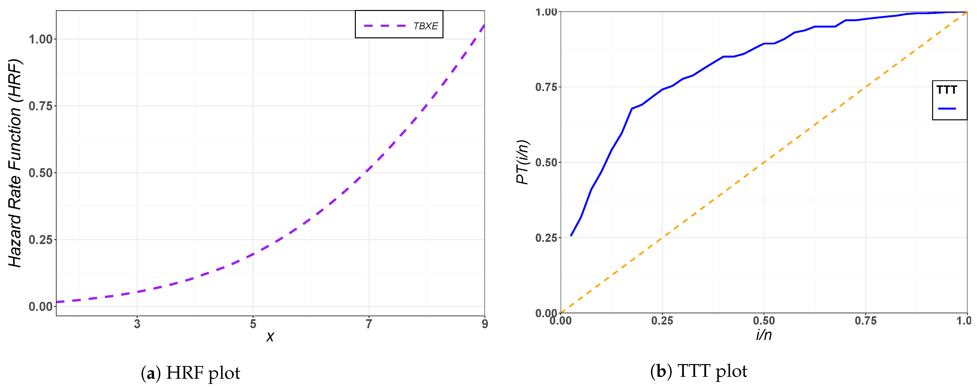
The fitted PDF and CDF plots for the TBXE model and other fitted models for the first and second data sets are depicted in Figure 3 and Figure 4, respectively. The HRF plot of the TBXE and total time on test (TTT) plot for the first and second data sets are depicted in Figure 5 and Figure 6, respectively. The TTT plot can be use for identifying the behavior of the HRF of the data. Figure 7 and Figure 8 provide the plots of the probability–probability (PP) of the TBXE model and other fitted models for the two data sets, respectively.

9. Conclusions

In this article, a new two-parameter generator, called transmuted Burr X generator (TBX-G), was proposed to extend the Burr X-G class and provide more flexibility in fitting real-life data. Two special sub-models, TBX-exponential (TBXE) and TBX-log-logistic (TBXLL) distributions, were studied. The structural properties of the TBX-G family were provided. We discussed eight estimation approaches to estimating the TBXE parameters. Numerical simulations were conducted to compare the eight estimation methods to determine the more accurate estimation methods based on partial and overall ranks. Our study showed that the Anderson–Darling estimation method is the best approach for estimating TBXE parameters. Using two real-life engineering data sets, we illustrated the importance and flexibility of the TBXE distribution compared with their competing existing models. The analyzed data showed that the special cases of the new family are capable of modeling right- and left-skewed data and outperform the existing competing models. The research in the current paper can be extended in several ways. For example, Bayesian estimation based on complete and censored samples could be explored to estimate the parameters of the special models of the TBX-G family. A bivariate family of distributions can be proposed to extended the univariate TBX-G family; a regression model based on the TBXE model can be developed with extensive study for estimating its parameters along with detailed sensitivity analysis.

Author Contributions

Funding acquisition and investigation, A.A.A.-B.; methodology, A.A.A.-B., I.E. and A.M.G.; formal analysis, I.E.; writing—original draft, A.M.G. and A.Z.A.; software and supervision, H.A.-M.; project administration and resources, A.Z.A.; writing—review & editing, H.A.-M., A.Z.A. and A.M.S. contributed equally to this work. All authors have read and agreed to the published version of the manuscript.

Funding

This project was supported by Researchers Supporting Project number (RSP- 2020/156) King Saud University, Riyadh, Saudi Arabia.

Acknowledgments

The authors would like to thank the Editorial Board and the three anonymous reviewers for their constructive comments that greatly improved the final version of the paper. This work was supported by King Saud University (KSU). The authors, therefore, gratefully acknowledges KSU for technical and financial support.

Conflicts of Interest

The authors declare no conflict of interest.

Appendix A

Table A1. Simulation results for Θ = ( β = 4.00 , φ = 3.00 , ρ = 0.50 ) .
nEst.Est. Par.WLSEOLSEMLEMPSECVMEADERADEPCE
50 B I A S β ^ 0.19636 { 6 } 0.21275 { 7 } 0.18543 { 4 } 0.17595 { 3 } 0.21916 { 8 } 0.19164 { 5 } 0.17161 { 1 } 0.17453 { 2 }
φ ^ 0.21998 { 5 } 0.23951 { 6 } 0.20825 { 2 } 0.21213 { 4 } 0.24984 { 7 } 0.21078 { 3 } 0.25254 { 8 } 0.20804 { 1 }
ρ ^ 0.21331 { 4 } 0.23100 { 6 } 0.26063 { 8 } 0.17950 { 1 } 0.23851 { 7 } 0.20903 { 3 } 0.22077 { 5 } 0.19923 { 2 }
MSE β ^ 0.05914 { 6 } 0.06887 { 7 } 0.05158 { 4 } 0.04692 { 3 } 0.07376 { 8 } 0.05552 { 5 } 0.04517 { 1 } 0.04519 { 2 }
φ ^ 0.08234 { 5 } 0.10155 { 6 } 0.07567 { 3 } 0.07208 { 2 } 0.11424 { 8 } 0.07727 { 4 } 0.11065 { 7 } 0.06906 { 1 }
ρ ^ 0.07429 { 2 } 0.08027 { 6 } 0.11301 { 8 } 0.07695 { 4 } 0.07510 { 3 } 0.06959 { 1 } 0.10006 { 7 } 0.07885 { 5 }
MRE β ^ 0.06545 { 6 } 0.07092 { 7 } 0.06181 { 4 } 0.05865 { 3 } 0.07305 { 8 } 0.06388 { 5 } 0.05720 { 1 } 0.05818 { 2 }
φ ^ 0.14665 { 5 } 0.15968 { 6 } 0.13883 { 2 } 0.14142 { 4 } 0.16656 { 7 } 0.14052 { 3 } 0.16836 { 8 } 0.13869 { 1 }
ρ ^ 0.28442 { 4 } 0.30800 { 6 } 0.34751 { 8 } 0.23934 { 1 } 0.31801 { 7 } 0.27871 { 3 } 0.29436 { 5 } 0.26564 { 2 }
R a n k s 43 { 5 } 57 { 7 } 43 { 5 } 25 { 2 } 63 { 8 } 32 { 3 } 43 { 5 } 18 { 1 }
150 B I A S β ^ 0.15710 { 5 } 0.17322 { 7 } 0.15884 { 6 } 0.12565 { 1 } 0.18034 { 8 } 0.15570 { 4 } 0.13677 { 3 } 0.13282 { 2 }
φ ^ 0.12101 { 5 } 0.13452 { 6 } 0.11753 { 2 } 0.11982 { 4 } 0.14030 { 8 } 0.11920 { 3 } 0.13563 { 7 } 0.11717 { 1 }
ρ ^ 0.18741 { 5 } 0.20764 { 6 } 0.22152 { 8 } 0.12997 { 1 } 0.21430 { 7 } 0.18247 { 4 } 0.18219 { 3 } 0.15328 { 2 }
MSE β ^ 0.03503 { 5 } 0.04177 { 7 } 0.03595 { 6 } 0.02430 { 1 } 0.04524 { 8 } 0.03452 { 4 } 0.02731 { 3 } 0.02644 { 2 }
φ ^ 0.02324 { 5 } 0.02892 { 6 } 0.02312 { 4 } 0.02206 { 2 } 0.03207 { 8 } 0.02259 { 3 } 0.02988 { 7 } 0.02172 { 1 }
ρ ^ 0.04492 { 4 } 0.05253 { 5 } 0.07756 { 8 } 0.03102 { 1 } 0.05505 { 6 } 0.04331 { 3 } 0.05615 { 7 } 0.04073 { 2 }
MRE β ^ 0.05237 { 5 } 0.05774 { 7 } 0.05295 { 6 } 0.04188 { 1 } 0.06011 { 8 } 0.05190 { 4 } 0.04559 { 3 } 0.04427 { 2 }
φ ^ 0.08067 { 5 } 0.08968 { 6 } 0.07835 { 2 } 0.07988 { 4 } 0.09353 { 8 } 0.07947 { 3 } 0.09042 { 7 } 0.07811 { 1 }
ρ ^ 0.24988 { 5 } 0.27685 { 6 } 0.29536 { 8 } 0.17330 { 1 } 0.28573 { 7 } 0.24330 { 4 } 0.24292 { 3 } 0.20438 { 2 }
R a n k s 44 { 5 } 56 { 7 } 50 { 6 } 16 { 2 } 68 { 8 } 32 { 3 } 43 { 4 } 15 { 1 }
300 B I A S β ^ 0.14168 { 6 } 0.15813 { 7 } 0.14054 { 5 } 0.09908 { 1 } 0.16119 { 8 } 0.13741 { 4 } 0.12501 { 3 } 0.11371 { 2 }
φ ^ 0.08811 { 4 } 0.09818 { 8 } 0.08407 { 1 } 0.08413 { 2 } 0.09579 { 6 } 0.08833 { 5 } 0.09734 { 7 } 0.08436 { 3 }
ρ ^ 0.17485 { 5 } 0.19747 { 7 } 0.19203 { 6 } 0.10694 { 1 } 0.20235 { 8 } 0.17178 { 4 } 0.16102 { 3 } 0.13399 { 2 }
MSE β ^ 0.02768 { 5 } 0.03321 { 7 } 0.02827 { 6 } 0.01618 { 1 } 0.03429 { 8 } 0.02637 { 4 } 0.02269 { 3 } 0.01979 { 2 }
φ ^ 0.01218 { 4 } 0.01508 { 8 } 0.01106 { 3 } 0.01086 { 2 } 0.01461 { 6 } 0.01225 { 5 } 0.01491 { 7 } 0.01085 { 1 }
ρ ^ 0.03901 { 4 } 0.04688 { 6 } 0.05677 { 8 } 0.01980 { 1 } 0.04891 { 7 } 0.03848 { 3 } 0.03914 { 5 } 0.02954 { 2 }
MRE β ^ 0.04723 { 6 } 0.05271 { 7 } 0.04685 { 5 } 0.03303 { 1 } 0.05373 { 8 } 0.04580 { 4 } 0.04167 { 3 } 0.03790 { 2 }
φ ^ 0.05874 { 4 } 0.06545 { 8 } 0.05604 { 1 } 0.05609 { 2 } 0.06386 { 6 } 0.05889 { 5 } 0.06489 { 7 } 0.05624 { 3 }
ρ ^ 0.23313 { 5 } 0.26329 { 7 } 0.25604 { 6 } 0.14259 { 1 } 0.26980 { 8 } 0.22904 { 4 } 0.21469 { 3 } 0.17866 { 2 }
R a n k s 43 { 6 } 65 { 7.5 } 41 { 4.5 } 12 { 1 } 65 { 7.5 } 38 { 3 } 41 { 4.5 } 19 { 2 }
400 B I A S β ^ 0.13391 { 5 } 0.15251 { 7 } 0.13510 { 6 } 0.09080 { 1 } 0.15666 { 8 } 0.13047 { 4 } 0.12093 { 3 } 0.10884 { 2 }
φ ^ 0.07563 { 4 } 0.08448 { 6 } 0.07213 { 1 } 0.07391 { 2 } 0.08568 { 8 } 0.07616 { 5 } 0.08505 { 7 } 0.07470 { 3 }
ρ ^ 0.16832 { 5 } 0.19117 { 7 } 0.18504 { 6 } 0.10058 { 1 } 0.19771 { 8 } 0.16261 { 4 } 0.15459 { 3 } 0.12992 { 2 }
MSE β ^ 0.02444 { 5 } 0.03037 { 7 } 0.02610 { 6 } 0.01392 { 1 } 0.03182 { 8 } 0.02339 { 4 } 0.02103 { 3 } 0.01810 { 2 }
φ ^ 0.00897 { 4 } 0.01125 { 7 } 0.00811 { 1 } 0.00826 { 2 } 0.01171 { 8 } 0.00902 { 5 } 0.01124 { 6 } 0.00858 { 3 }
ρ ^ 0.03630 { 5 } 0.04431 { 6 } 0.05245 { 8 } 0.01813 { 1 } 0.04707 { 7 } 0.03456 { 4 } 0.03418 { 3 } 0.02775 { 2 }
MRE β ^ 0.04464 { 5 } 0.05084 { 7 } 0.04503 { 6 } 0.03027 { 1 } 0.05222 { 8 } 0.04349 { 4 } 0.04031 { 3 } 0.03628 { 2 }
φ ^ 0.05042 { 4 } 0.05632 { 6 } 0.04808 { 1 } 0.04928 { 2 } 0.05712 { 8 } 0.05077 { 5 } 0.05670 { 7 } 0.04980 { 3 }
ρ ^ 0.22443 { 5 } 0.25489 { 7 } 0.24672 { 6 } 0.13411 { 1 } 0.26361 { 8 } 0.21682 { 4 } 0.20612 { 3 } 0.17322 { 2 }
R a n k s 42 { 6 } 60 { 7 } 41 { 5 } 12 { 1 } 71 { 8 } 39 { 4 } 38 { 3 } 21 { 2 }
Table A2. Simulation results for Θ = ( β = 0.75 , φ = 1.00 , ρ = 0.30 ) .
nEst.Est. Par.WLSEOLSEMLEMPSECVMEADERADEPCE
50 B I A S β ^ 0.05497 { 2 } 0.05640 { 4 } 0.12286 { 8 } 0.05995 { 7 } 0.05658 { 5 } 0.05258 { 1 } 0.05589 { 3 } 0.05901 { 6 }
φ ^ 0.18671 { 5 } 0.19952 { 8 } 0.18265 { 4 } 0.19242 { 6 } 0.19256 { 7 } 0.17964 { 3 } 0.17932 { 2 } 0.17890 { 1 }
ρ ^ 0.45325 { 7 } 0.45293 { 6 } 0.36028 { 1 } 0.46707 { 8 } 0.43161 { 2 } 0.44144 { 4 } 0.43901 { 3 } 0.44752 { 5 }
MSE β ^ 0.00458 { 2 } 0.00484 { 4 } 0.06117 { 8 } 0.00539 { 7 } 0.00502 { 5 } 0.00426 { 1 } 0.00482 { 3 } 0.00523 { 6 }
φ ^ 0.05358 { 4 } 0.05969 { 8 } 0.05481 { 5 } 0.05910 { 7 } 0.05786 { 6 } 0.05004 { 3 } 0.04942 { 2 } 0.04926 { 1 }
ρ ^ 0.28156 { 7 } 0.27771 { 6 } 0.20268 { 1 } 0.31328 { 8 } 0.25651 { 3 } 0.27391 { 5 } 0.25203 { 2 } 0.27031 { 4 }
MRE β ^ 0.07329 { 2 } 0.07520 { 4 } 0.16382 { 8 } 0.07994 { 7 } 0.07544 { 5 } 0.07011 { 1 } 0.07452 { 3 } 0.07868 { 6 }
φ ^ 0.18671 { 5 } 0.19952 { 8 } 0.18265 { 4 } 0.19242 { 6 } 0.19256 { 7 } 0.17964 { 3 } 0.17932 { 2 } 0.17890 { 1 }
ρ ^ 1.51082 { 7 } 1.50977 { 6 } 1.20093 { 1 } 1.55691 { 8 } 1.43871 { 2 } 1.47146 { 4 } 1.46337 { 3 } 1.49174 { 5 }
R a n k s 41 { 5 } 54 { 7 } 40 { 4 } 64 { 8 } 42 { 6 } 25 { 2 } 23 { 1 } 35 { 3 }
150 B I A S β ^ 0.04009 { 2 } 0.04205 { 5 } 0.11198 { 8 } 0.04709 { 7 } 0.04048 { 3 } 0.03960 { 1 } 0.04131 { 4 } 0.04590 { 6 }
φ ^ 0.12091 { 3 } 0.13461 { 8 } 0.12843 { 6 } 0.12374 { 4 } 0.13198 { 7 } 0.11710 { 2 } 0.12416 { 5 } 0.11212 { 1 }
ρ ^ 0.35004 { 3 } 0.37236 { 7 } 0.29516 { 1 } 0.37953 { 8 } 0.36006 { 6 } 0.34178 { 2 } 0.35325 { 4 } 0.35771 { 5 }
MSE β ^ 0.00237 { 2 } 0.00258 { 5 } 0.06064 { 8 } 0.00343 { 7 } 0.00244 { 3 } 0.00233 { 1 } 0.00249 { 4 } 0.00313 { 6 }
φ ^ 0.02473 { 3 } 0.02959 { 6 } 0.03219 { 8 } 0.03017 { 7 } 0.02797 { 5 } 0.02330 { 2 } 0.02487 { 4 } 0.02248 { 1 }
ρ ^ 0.18034 { 4 } 0.19931 { 7 } 0.14295 { 1 } 0.23276 { 8 } 0.18784 { 6 } 0.17404 { 2 } 0.17747 { 3 } 0.18218 { 5 }
MRE β ^ 0.05345 { 2 } 0.05606 { 5 } 0.14931 { 8 } 0.06279 { 7 } 0.05397 { 3 } 0.05280 { 1 } 0.05507 { 4 } 0.06119 { 6 }
φ ^ 0.12091 { 3 } 0.13461 { 8 } 0.12843 { 6 } 0.12374 { 4 } 0.13198 { 7 } 0.11710 { 2 } 0.12416 { 5 } 0.11212 { 1 }
ρ ^ 1.16680 { 3 } 1.24122 { 7 } 0.98386 { 1 } 1.26510 { 8 } 1.20022 { 6 } 1.13928 { 2 } 1.17749 { 4 } 1.19237 { 5 }
R a n k s 25 { 2 } 58 { 7 } 47 { 6 } 60 { 8 } 46 { 5 } 15 { 1 } 37 { 4 } 36 { 3 }
300 B I A S β ^ 0.03340 { 2 } 0.03573 { 5 } 0.10479 { 8 } 0.03867 { 7 } 0.03516 { 4 } 0.03338 { 1 } 0.03402 { 3 } 0.03861 { 6 }
φ ^ 0.08292 { 4 } 0.09920 { 7 } 0.10216 { 8 } 0.08232 { 3 } 0.09493 { 6 } 0.07933 { 2 } 0.09348 { 5 } 0.07566 { 1 }
ρ ^ 0.27273 { 3 } 0.30794 { 8 } 0.24152 { 1 } 0.29007 { 6 } 0.29730 { 7 } 0.26593 { 2 } 0.28359 { 5 } 0.28155 { 4 }
MSE β ^ 0.00165 { 1 } 0.00182 { 5 } 0.05921 { 8 } 0.00250 { 7 } 0.00177 { 4 } 0.00166 { 2 } 0.00175 { 3 } 0.00234 { 6 }
φ ^ 0.01235 { 3 } 0.01759 { 7 } 0.02490 { 8 } 0.01466 { 4 } 0.01592 { 6 } 0.01128 { 2 } 0.01490 { 5 } 0.01074 { 1 }
ρ ^ 0.11123 { 3 } 0.14005 { 7 } 0.09957 { 1 } 0.14753 { 8 } 0.13195 { 6 } 0.10660 { 2 } 0.12083 { 5 } 0.12015 { 4 }
MRE β ^ 0.04453 { 2 } 0.04764 { 5 } 0.13972 { 8 } 0.05156 { 7 } 0.04688 { 4 } 0.04451 { 1 } 0.04536 { 3 } 0.05148 { 6 }
φ ^ 0.08292 { 4 } 0.09920 { 7 } 0.10216 { 8 } 0.08232 { 3 } 0.09493 { 6 } 0.07933 { 2 } 0.09348 { 5 } 0.07566 { 1 }
ρ ^ 0.90912 { 3 } 1.02648 { 8 } 0.80507 { 1 } 0.96689 { 6 } 0.99099 { 7 } 0.88642 { 2 } 0.94529 { 5 } 0.93849 { 4 }
R a n k s 25 { 2 } 59 { 8 } 51 { 6.5 } 51 { 6.5 } 50 { 5 } 16 { 1 } 39 { 4 } 33 { 3 }
400 B I A S β ^ 0.03047 { 1 } 0.03410 { 5 } 0.10898 { 8 } 0.03605 { 7 } 0.03313 { 4 } 0.03063 { 2 } 0.03138 { 3 } 0.03548 { 6 }
φ ^ 0.07037 { 3 } 0.08384 { 7 } 0.09425 { 8 } 0.07172 { 4 } 0.08313 { 6 } 0.06830 { 2 } 0.08171 { 5 } 0.06501 { 1 }
ρ ^ 0.24256 { 3 } 0.28045 { 8 } 0.22193 { 1 } 0.26182 { 6 } 0.27334 { 7 } 0.24062 { 2 } 0.25646 { 5 } 0.25503 { 4 }
MSE β ^ 0.00140 { 1 } 0.00165 { 5 } 0.06368 { 8 } 0.00227 { 7 } 0.00156 { 4 } 0.00143 { 2 } 0.00151 { 3 } 0.00207 { 6 }
φ ^ 0.00870 { 3 } 0.01319 { 7 } 0.02278 { 8 } 0.01143 { 4 } 0.01232 { 6 } 0.00830 { 2 } 0.01149 { 5 } 0.00759 { 1 }
ρ ^ 0.08852 { 3 } 0.11744 { 7 } 0.08065 { 1 } 0.12744 { 8 } 0.11016 { 6 } 0.08787 { 2 } 0.10026 { 5 } 0.09939 { 4 }
MRE β ^ 0.04062 { 1 } 0.04547 { 5 } 0.14531 { 8 } 0.04807 { 7 } 0.04418 { 4 } 0.04084 { 2 } 0.04184 { 3 } 0.04730 { 6 }
φ ^ 0.07037 { 3 } 0.08384 { 7 } 0.09425 { 8 } 0.07172 { 4 } 0.08313 { 6 } 0.06830 { 2 } 0.08171 { 5 } 0.06501 { 1 }
ρ ^ 0.80852 { 3 } 0.93485 { 8 } 0.73977 { 1 } 0.87275 { 6 } 0.91113 { 7 } 0.80206 { 2 } 0.85486 { 5 } 0.85011 { 4 }
R a n k s 21 { 2 } 59 { 8 } 51 { 6 } 53 { 7 } 50 { 5 } 18 { 1 } 39 { 4 } 33 { 3 }
Table A3. Simulation results for Θ = ( β = 1.00 , φ = 1.50 , ρ = 0.50 ) .
nEst.Est. Par.WLSEOLSEMLEMPSECVMEADERADEPCE
50 B I A S β ^ 0.05035 { 3 } 0.05552 { 8 } 0.04297 { 1 } 0.05536 { 7 } 0.05254 { 4 } 0.04891 { 2 } 0.05339 { 5 } 0.05514 { 6 }
φ ^ 0.29167 { 4 } 0.28304 { 1 } 0.31787 { 7 } 0.29207 { 5 } 0.30329 { 6 } 0.28430 { 2 } 0.34093 { 8 } 0.28602 { 3 }
ρ ^ 0.33131 { 3 } 0.32834 { 2 } 0.35874 { 6 } 0.35066 { 4 } 0.31656 { 1 } 0.35480 { 5 } 0.36839 { 7 } 0.36906 { 8 }
MSE β ^ 0.00408 { 3 } 0.00493 { 6 } 0.00299 { 1 } 0.00516 { 8 } 0.00438 { 4 } 0.00386 { 2 } 0.00464 { 5 } 0.00504 { 7 }
φ ^ 0.12644 { 4 } 0.12748 { 5 } 0.15880 { 6 } 0.12547 { 3 } 0.15880 { 7 } 0.12211 { 2 } 0.20389 { 8 } 0.11612 { 1 }
ρ ^ 0.21337 { 2 } 0.22110 { 4 } 0.22018 { 3 } 0.24269 { 6 } 0.20040 { 1 } 0.23352 { 5 } 0.27493 { 8 } 0.26648 { 7 }
MRE β ^ 0.05035 { 3 } 0.05552 { 8 } 0.04297 { 1 } 0.05536 { 7 } 0.05254 { 4 } 0.04891 { 2 } 0.05339 { 5 } 0.05514 { 6 }
φ ^ 0.19444 { 4 } 0.18870 { 1 } 0.21191 { 7 } 0.19471 { 5 } 0.20220 { 6 } 0.18953 { 2 } 0.22729 { 8 } 0.19068 { 3 }
ρ ^ 0.66262 { 6 } 0.65668 { 7 } 0.71747 { 3 } 0.70131 { 5 } 0.63312 { 8 } 0.70959 { 4 } 0.73679 { 2 } 0.73812 { 1 }
R a n k s 32 { 2 } 42 { 5.5 } 35 { 3 } 50 { 7 } 41 { 4 } 26 { 1 } 56 { 8 } 42 { 5.5 }
150 B I A S β ^ 0.02975 { 3 } 0.03327 { 8 } 0.02726 { 1 } 0.02983 { 4 } 0.03186 { 6 } 0.02862 { 2 } 0.03122 { 5 } 0.03264 { 7 }
φ ^ 0.23920 { 4 } 0.23366 { 1 } 0.27688 { 8 } 0.23413 { 2 } 0.23592 { 3 } 0.24001 { 5 } 0.26743 { 7 } 0.25938 { 6 }
ρ ^ 0.28846 { 3 } 0.29146 { 4 } 0.30545 { 6 } 0.26143 { 1 } 0.28262 { 2 } 0.29478 { 5 } 0.30600 { 7 } 0.31586 { 8 }
MSE β ^ 0.00158 { 3 } 0.00192 { 7 } 0.00141 { 1 } 0.00176 { 5 } 0.00171 { 4 } 0.00146 { 2 } 0.00178 { 6 } 0.00210 { 8 }
φ ^ 0.08421 { 4 } 0.08040 { 1 } 0.11430 { 8 } 0.08243 { 2 } 0.08393 { 3 } 0.08503 { 5 } 0.10408 { 7 } 0.09454 { 6 }
ρ ^ 0.15845 { 2 } 0.17227 { 6 } 0.16797 { 5 } 0.13798 { 1 } 0.16104 { 4 } 0.16081 { 3 } 0.19270 { 8 } 0.19160 { 7 }
MRE β ^ 0.02975 { 3 } 0.03327 { 8 } 0.02726 { 1 } 0.02983 { 4 } 0.03186 { 6 } 0.02862 { 2 } 0.03122 { 5 } 0.03264 { 7 }
φ ^ 0.15947 { 4 } 0.15577 { 1 } 0.18459 { 8 } 0.15609 { 2 } 0.15728 { 3 } 0.16001 { 5 } 0.17829 { 7 } 0.17292 { 6 }
ρ ^ 0.57691 { 6 } 0.58292 { 5 } 0.61090 { 3 } 0.52286 { 8 } 0.56525 { 7 } 0.58956 { 4 } 0.61200 { 2 } 0.63173 { 1 }
R a n k s 32 { 2 } 41 { 5.5 } 41 { 5.5 } 29 { 1 } 38 { 4 } 33 { 3 } 54 { 7 } 56 { 8 }
300 B I A S β ^ 0.02057 { 4 } 0.02308 { 8 } 0.01927 { 1 } 0.02033 { 3 } 0.02295 { 7 } 0.02022 { 2 } 0.02178 { 5 } 0.02237 { 6 }
φ ^ 0.21577 { 3 } 0.21204 { 2 } 0.24170 { 8 } 0.19276 { 1 } 0.21722 { 5 } 0.21650 { 4 } 0.23983 { 7 } 0.23761 { 6 }
ρ ^ 0.24968 { 3 } 0.25177 { 4 } 0.25882 { 6 } 0.20385 { 1 } 0.25595 { 5 } 0.24951 { 2 } 0.26351 { 7 } 0.27189 { 8 }
MSE β ^ 0.00080 { 3 } 0.00098 { 7 } 0.00078 { 2 } 0.00084 { 4 } 0.00095 { 6 } 0.00078 { 1 } 0.00094 { 5 } 0.00107 { 8 }
φ ^ 0.07045 { 3 } 0.07018 { 2 } 0.08680 { 8 } 0.06161 { 1 } 0.07305 { 5 } 0.07172 { 4 } 0.08598 { 7 } 0.07932 { 6 }
ρ ^ 0.11550 { 3 } 0.12742 { 5 } 0.11994 { 4 } 0.08816 { 1 } 0.13031 { 6 } 0.11490 { 2 } 0.14299 { 8 } 0.13345 { 7 }
MRE β ^ 0.02057 { 4 } 0.02308 { 8 } 0.01927 { 1 } 0.02033 { 3 } 0.02295 { 7 } 0.02022 { 2 } 0.02178 { 5 } 0.02237 { 6 }
φ ^ 0.14385 { 3 } 0.14136 { 2 } 0.16113 { 8 } 0.12850 { 1 } 0.14481 { 5 } 0.14433 { 4 } 0.15989 { 7 } 0.15841 { 6 }
ρ ^ 0.49937 { 6 } 0.50355 { 5 } 0.51764 { 3 } 0.40769 { 8 } 0.51189 { 4 } 0.49902 { 7 } 0.52702 { 2 } 0.54379 { 1 }
R a n k s 32 { 3 } 43 { 5 } 41 { 4 } 23 { 1 } 50 { 6 } 28 { 2 } 53 { 7 } 54 { 8 }
400 B I A S β ^ 0.01762 { 4 } 0.01995 { 7 } 0.01637 { 1 } 0.01695 { 2 } 0.02002 { 8 } 0.01738 { 3 } 0.01852 { 6 } 0.01808 { 5 }
φ ^ 0.20161 { 2 } 0.20271 { 3 } 0.22685 { 7 } 0.17186 { 1 } 0.20517 { 4 } 0.20973 { 5 } 0.23420 { 8 } 0.22643 { 6 }
ρ ^ 0.23165 { 2 } 0.23820 { 3 } 0.24259 { 6 } 0.18034 { 1 } 0.24118 { 5 } 0.24083 { 4 } 0.25448 { 8 } 0.24669 { 7 }
MSE β ^ 0.00060 { 4 } 0.00074 { 7 } 0.00055 { 1 } 0.00058 { 2 } 0.00075 { 8 } 0.00058 { 3 } 0.00068 { 5 } 0.00068 { 6 }
φ ^ 0.06316 { 2 } 0.06560 { 3 } 0.07633 { 7 } 0.05238 { 1 } 0.06776 { 5 } 0.06746 { 4 } 0.08393 { 8 } 0.07204 { 6 }
ρ ^ 0.09863 { 2 } 0.11344 { 6 } 0.09926 { 3 } 0.07007 { 1 } 0.11544 { 7 } 0.10288 { 5 } 0.12934 { 8 } 0.10262 { 4 }
MRE β ^ 0.01762 { 4 } 0.01995 { 7 } 0.01637 { 1 } 0.01695 { 2 } 0.02002 { 8 } 0.01738 { 3 } 0.01852 { 6 } 0.01808 { 5 }
φ ^ 0.13441 { 2 } 0.13514 { 3 } 0.15123 { 7 } 0.11457 { 1 } 0.13678 { 4 } 0.13982 { 5 } 0.15614 { 8 } 0.15095 { 6 }
ρ ^ 0.46331 { 7 } 0.47639 { 6 } 0.48518 { 3 } 0.36067 { 8 } 0.48237 { 4 } 0.48167 { 5 } 0.50896 { 1 } 0.49337 { 2 }
R a n k s 29 { 2 } 45 { 5 } 36 { 3 } 19 { 1 } 53 { 7 } 37 { 4 } 58 { 8 } 47 { 6 }
Table A4. Simulation results for Θ = ( β = 4.00 , φ = 3.00 , ρ = 0.50 ) .
nEst.Est. Par.WLSEOLSEMLEMPSECVMEADERADEPCE
50 B I A S β ^ 0.19731 { 6 } 0.19039 { 5 } 0.19888 { 7 } 0.20764 { 8 } 0.18884 { 3 } 0.18071 { 1 } 0.18159 { 2 } 0.18985 { 4 }
φ ^ 0.53813 { 3 } 0.59920 { 7 } 0.51596 { 1 } 0.55371 { 5 } 0.59963 { 8 } 0.53084 { 2 } 0.57907 { 6 } 0.55163 { 4 }
ρ ^ 0.30609 { 1 } 0.31791 { 3 } 0.36726 { 8 } 0.33360 { 5 } 0.31449 { 2 } 0.33390 { 6 } 0.33659 { 7 } 0.33122 { 4 }
MSE β ^ 0.05987 { 7 } 0.05419 { 4 } 0.05825 { 6 } 0.06508 { 8 } 0.05477 { 5 } 0.04877 { 2 } 0.04772 { 1 } 0.05335 { 3 }
φ ^ 0.48370 { 5 } 0.59604 { 7 } 0.44791 { 1 } 0.47082 { 2 } 0.68934 { 8 } 0.47095 { 3 } 0.56015 { 6 } 0.47440 { 4 }
ρ ^ 0.18164 { 1 } 0.19679 { 4 } 0.22272 { 7 } 0.21058 { 6 } 0.18211 { 2 } 0.19879 { 5 } 0.19280 { 3 } 0.22724 { 8 }
MRE β ^ 0.04933 { 6 } 0.04760 { 5 } 0.04972 { 7 } 0.05191 { 8 } 0.04721 { 3 } 0.04518 { 1 } 0.04540 { 2 } 0.04746 { 4 }
φ ^ 0.17938 { 3 } 0.19973 { 7 } 0.17199 { 1 } 0.18457 { 5 } 0.19988 { 8 } 0.17695 { 2 } 0.19302 { 6 } 0.18388 { 4 }
ρ ^ 0.61217 { 1 } 0.63581 { 3 } 0.73452 { 8 } 0.66720 { 5 } 0.62897 { 2 } 0.66780 { 6 } 0.67318 { 7 } 0.66244 { 4 }
R a n k s 33 { 2 } 45 { 6 } 46 { 7 } 52 { 8 } 41 { 5 } 28 { 1 } 40 { 4 } 39 { 3 }
150 B I A S β ^ 0.15882 { 5 } 0.15311 { 3 } 0.17073 { 8 } 0.16591 { 7 } 0.15488 { 4 } 0.15046 { 1 } 0.15118 { 2 } 0.16532 { 6 }
φ ^ 0.31194 { 3 } 0.35091 { 8 } 0.30593 { 1 } 0.32565 { 4 } 0.34698 { 7 } 0.30625 { 2 } 0.34351 { 5 } 0.34559 { 6 }
ρ ^ 0.26994 { 2 } 0.27685 { 4 } 0.31188 { 8 } 0.26536 { 1 } 0.27985 { 5 } 0.27392 { 3 } 0.29630 { 6 } 0.29923 { 7 }
MSE β ^ 0.03785 { 5 } 0.03564 { 3 } 0.04215 { 8 } 0.04114 { 7 } 0.03605 { 4 } 0.03362 { 2 } 0.03280 { 1 } 0.03889 { 6 }
φ ^ 0.16119 { 3 } 0.20217 { 7 } 0.15920 { 2 } 0.17820 { 4 } 0.19808 { 6 } 0.15711 { 1 } 0.18993 { 5 } 0.20356 { 8 }
ρ ^ 0.13687 { 3 } 0.14656 { 5 } 0.16829 { 7 } 0.13373 { 1 } 0.14492 { 4 } 0.13668 { 2 } 0.15203 { 6 } 0.17620 { 8 }
MRE β ^ 0.03971 { 5 } 0.03828 { 3 } 0.04268 { 8 } 0.04148 { 7 } 0.03872 { 4 } 0.03762 { 1 } 0.03779 { 2 } 0.04133 { 6 }
φ ^ 0.10398 { 3 } 0.11697 { 8 } 0.10198 { 1 } 0.10855 { 4 } 0.11566 { 7 } 0.10208 { 2 } 0.11450 { 5 } 0.11520 { 6 }
ρ ^ 0.53987 { 2 } 0.55370 { 4 } 0.62376 { 8 } 0.53071 { 1 } 0.55970 { 5 } 0.54783 { 3 } 0.59260 { 6 } 0.59845 { 7 }
R a n k s 31 { 2 } 45 { 5 } 51 { 7 } 36 { 3 } 46 { 6 } 17 { 1 } 38 { 4 } 60 { 8 }
300 B I A S β ^ 0.13729 { 3 } 0.13971 { 6 } 0.14968 { 7 } 0.13379 { 1 } 0.13866 { 5 } 0.13756 { 4 } 0.13547 { 2 } 0.15046 { 8 }
φ ^ 0.21885 { 3 } 0.25206 { 8 } 0.21485 { 1 } 0.22846 { 4 } 0.24644 { 7 } 0.21803 { 2 } 0.24595 { 6 } 0.23913 { 5 }
ρ ^ 0.23687 { 2 } 0.24633 { 5 } 0.26974 { 8 } 0.21418 { 1 } 0.24264 { 3 } 0.24323 { 4 } 0.25122 { 6 } 0.25767 { 7 }
MSE β ^ 0.02934 { 4 } 0.03081 { 6 } 0.03229 { 8 } 0.02882 { 2 } 0.02997 { 5 } 0.02891 { 3 } 0.02725 { 1 } 0.03224 { 7 }
φ ^ 0.07862 { 1 } 0.10393 { 8 } 0.08288 { 3 } 0.09014 { 4 } 0.09928 { 6 } 0.07903 { 2 } 0.09770 { 5 } 0.10222 { 7 }
ρ ^ 0.09966 { 2 } 0.11314 { 6 } 0.12169 { 7 } 0.08886 { 1 } 0.10770 { 4 } 0.10365 { 3 } 0.10801 { 5 } 0.12177 { 8 }
MRE β ^ 0.03432 { 3 } 0.03493 { 6 } 0.03742 { 7 } 0.03345 { 1 } 0.03466 { 5 } 0.03439 { 4 } 0.03387 { 2 } 0.03761 { 8 }
φ ^ 0.07295 { 3 } 0.08402 { 8 } 0.07162 { 1 } 0.07615 { 4 } 0.08215 { 7 } 0.07268 { 2 } 0.08198 { 6 } 0.07971 { 5 }
ρ ^ 0.47375 { 2 } 0.49266 { 5 } 0.53948 { 8 } 0.42837 { 1 } 0.48527 { 3 } 0.48645 { 4 } 0.50244 { 6 } 0.51533 { 7 }
R a n k s 23 { 2 } 58 { 7 } 50 { 6 } 19 { 1 } 45 { 5 } 28 { 3 } 39 { 4 } 62 { 8 }
400 B I A S β ^ 0.12955 { 2 } 0.13443 { 5 } 0.14106 { 7 } 0.12071 { 1 } 0.13453 { 6 } 0.13057 { 4 } 0.13033 { 3 } 0.14511 { 8 }
φ ^ 0.18975 { 2 } 0.21345 { 6 } 0.19049 { 3 } 0.19472 { 4 } 0.21206 { 5 } 0.18833 { 1 } 0.21728 { 8 } 0.21407 { 7 }
ρ ^ 0.22180 { 2 } 0.22856 { 4 } 0.24961 { 8 } 0.18807 { 1 } 0.23376 { 5 } 0.22430 { 3 } 0.23983 { 6 } 0.24753 { 7 }
MSE β ^ 0.02645 { 3 } 0.02895 { 6 } 0.02922 { 7 } 0.02512 { 2 } 0.02869 { 5 } 0.02659 { 4 } 0.02508 { 1 } 0.02981 { 8 }
φ ^ 0.05886 { 2 } 0.07213 { 5 } 0.06428 { 3 } 0.06470 { 4 } 0.07299 { 6 } 0.05827 { 1 } 0.07631 { 7 } 0.08197 { 8 }
ρ ^ 0.08643 { 2 } 0.09501 { 4 } 0.10507 { 7 } 0.06945 { 1 } 0.09836 { 6 } 0.08732 { 3 } 0.09806 { 5 } 0.10945 { 8 }
MRE β ^ 0.03239 { 2 } 0.03361 { 5 } 0.03527 { 7 } 0.03018 { 1 } 0.03363 { 6 } 0.03264 { 4 } 0.03258 { 3 } 0.03628 { 8 }
φ ^ 0.06325 { 2 } 0.07115 { 6 } 0.06350 { 3 } 0.06491 { 4 } 0.07069 { 5 } 0.06278 { 1 } 0.07243 { 8 } 0.07136 { 7 }
ρ ^ 0.44360 { 2 } 0.45713 { 4 } 0.49922 { 8 } 0.37613 { 1 } 0.46751 { 5 } 0.44861 { 3 } 0.47965 { 6 } 0.49506 { 7 }
R a n k s 19 { 1.5 } 45 { 4 } 53 { 7 } 19 { 1.5 } 49 { 6 } 24 { 3 } 47 { 5 } 68 { 8 }
Table A5. Simulation results for Θ = ( β = 3.00 , φ = 1.50 , ρ = 0.30 ) .
nEst.Est. Par.WLSEOLSEMLEMPSECVMEADERADEPCE
50 B I A S β ^ 0.18133 { 3 } 0.18433 { 5 } 0.18363 { 4 } 0.20934 { 8 } 0.18114 { 2 } 0.17863 { 1 } 0.19393 { 6 } 0.19953 { 7 }
φ ^ 0.28939 { 5 } 0.30744 { 8 } 0.25388 { 1 } 0.29657 { 7 } 0.29633 { 6 } 0.27690 { 3 } 0.27375 { 2 } 0.28495 { 4 }
ρ ^ 0.44199 { 6 } 0.43180 { 4 } 0.37852 { 1 } 0.45771 { 8 } 0.41271 { 2 } 0.43542 { 5 } 0.42886 { 3 } 0.44375 { 7 }
MSE β ^ 0.05036 { 2 } 0.05183 { 4 } 0.05243 { 5 } 0.06610 { 8 } 0.05121 { 3 } 0.04928 { 1 } 0.05784 { 6 } 0.06001 { 7 }
φ ^ 0.12833 { 5 } 0.14235 { 8 } 0.10433 { 1 } 0.13678 { 6 } 0.13882 { 7 } 0.11821 { 3 } 0.11486 { 2 } 0.12357 { 4 }
ρ ^ 0.27523 { 6 } 0.26400 { 4 } 0.22207 { 1 } 0.30744 { 8 } 0.24580 { 3 } 0.27214 { 5 } 0.24481 { 2 } 0.27798 { 7 }
MRE β ^ 0.06044 { 3 } 0.06144 { 5 } 0.06121 { 4 } 0.06978 { 8 } 0.06038 { 2 } 0.05954 { 1 } 0.06464 { 6 } 0.06651 { 7 }
φ ^ 0.19293 { 5 } 0.20496 { 8 } 0.16925 { 1 } 0.19772 { 7 } 0.19755 { 6 } 0.18460 { 3 } 0.18250 { 2 } 0.18997 { 4 }
ρ ^ 1.47331 { 6 } 1.43933 { 4 } 1.26174 { 1 } 1.52570 { 8 } 1.37570 { 2 } 1.45140 { 5 } 1.42954 { 3 } 1.47918 { 7 }
R a n k s 41 { 5 } 50 { 6 } 19 { 1 } 68 { 8 } 33 { 4 } 27 { 2 } 32 { 3 } 54 { 7 }
150 B I A S β ^ 0.13707 { 4 } 0.13737 { 5 } 0.13607 { 2 } 0.16400 { 8 } 0.13413 { 1 } 0.13626 { 3 } 0.14497 { 6 } 0.15859 { 7 }
φ ^ 0.18302 { 4 } 0.20553 { 8 } 0.15974 { 1 } 0.18813 { 6 } 0.19877 { 7 } 0.17818 { 2 } 0.18784 { 5 } 0.17851 { 3 }
ρ ^ 0.35844 { 3 } 0.37134 { 6 } 0.31888 { 1 } 0.38499 { 8 } 0.36011 { 4 } 0.35320 { 2 } 0.36516 { 5 } 0.37802 { 7 }
MSE β ^ 0.02754 { 3 } 0.02769 { 4 } 0.02822 { 5 } 0.04115 { 8 } 0.02682 { 1 } 0.02725 { 2 } 0.03052 { 6 } 0.03687 { 7 }
φ ^ 0.05610 { 4 } 0.06732 { 7 } 0.04571 { 1 } 0.06803 { 8 } 0.06258 { 6 } 0.05307 { 2 } 0.05585 { 3 } 0.05768 { 5 }
ρ ^ 0.19029 { 4 } 0.20259 { 6 } 0.16497 { 1 } 0.23762 { 8 } 0.19279 { 5 } 0.18623 { 2 } 0.18641 { 3 } 0.20861 { 7 }
MRE β ^ 0.04569 { 4 } 0.04579 { 5 } 0.04536 { 2 } 0.05467 { 8 } 0.04471 { 1 } 0.04542 { 3 } 0.04832 { 6 } 0.05286 { 7 }
φ ^ 0.12202 { 4 } 0.13702 { 8 } 0.10649 { 1 } 0.12542 { 6 } 0.13251 { 7 } 0.11878 { 2 } 0.12523 { 5 } 0.11901 { 3 }
ρ ^ 1.19479 { 3 } 1.23781 { 6 } 1.06293 { 1 } 1.28331 { 8 } 1.20038 { 4 } 1.17733 { 2 } 1.21721 { 5 } 1.26007 { 7 }
R a n k s 33 { 3 } 55 { 7 } 15 { 1 } 68 { 8 } 36 { 4 } 20 { 2 } 44 { 5 } 53 { 6 }
300 B I A S β ^ 0.11743 { 3 } 0.12266 { 5 } 0.11418 { 1 } 0.13973 { 8 } 0.11954 { 4 } 0.11657 { 2 } 0.12401 { 6 } 0.13797 { 7 }
φ ^ 0.12724 { 4 } 0.14997 { 8 } 0.11519 { 1 } 0.12975 { 5 } 0.14593 { 7 } 0.12476 { 3 } 0.13767 { 6 } 0.12027 { 2 }
ρ ^ 0.28494 { 3 } 0.31225 { 8 } 0.26669 { 1 } 0.30087 { 5 } 0.30512 { 7 } 0.28132 { 2 } 0.29796 { 4 } 0.30306 { 6 }
MSE β ^ 0.02038 { 2 } 0.02152 { 5 } 0.02059 { 3 } 0.03159 { 8 } 0.02072 { 4 } 0.02014 { 1 } 0.02274 { 6 } 0.02895 { 7 }
φ ^ 0.02980 { 4 } 0.03939 { 8 } 0.02593 { 1 } 0.03634 { 6 } 0.03689 { 7 } 0.02872 { 3 } 0.03275 { 5 } 0.02804 { 2 }
ρ ^ 0.12405 { 3 } 0.14682 { 7 } 0.11700 { 1 } 0.15961 { 8 } 0.14086 { 6 } 0.12131 { 2 } 0.13154 { 4 } 0.13645 { 5 }
MRE β ^ 0.03914 { 3 } 0.04089 { 5 } 0.03806 { 1 } 0.04658 { 8 } 0.03985 { 4 } 0.03886 { 2 } 0.04134 { 6 } 0.04599 { 7 }
φ ^ 0.08483 { 4 } 0.09998 { 8 } 0.07679 { 1 } 0.08650 { 5 } 0.09729 { 7 } 0.08318 { 3 } 0.09178 { 6 } 0.08018 { 2 }
ρ ^ 0.94979 { 3 } 1.04084 { 8 } 0.88895 { 1 } 1.00289 { 5 } 1.01706 { 7 } 0.93775 { 2 } 0.99318 { 4 } 1.01020 { 6 }
R a n k s 29 { 3 } 62 { 8 } 11 { 1 } 58 { 7 } 53 { 6 } 20 { 2 } 47 { 5 } 44 { 4 }
400 B I A S β ^ 0.11102 { 3 } 0.11592 { 5 } 0.10638 { 1 } 0.12815 { 7 } 0.11325 { 4 } 0.11058 { 2 } 0.11710 { 6 } 0.12966 { 8 }
φ ^ 0.10711 { 5 } 0.12898 { 8 } 0.09874 { 1 } 0.10597 { 4 } 0.12609 { 7 } 0.10543 { 3 } 0.11885 { 6 } 0.09877 { 2 }
ρ ^ 0.26267 { 3 } 0.29093 { 8 } 0.24002 { 1 } 0.26530 { 4 } 0.28482 { 7 } 0.25982 { 2 } 0.27314 { 5 } 0.27768 { 6 }
MSE β ^ 0.01820 { 2 } 0.01915 { 5 } 0.01836 { 3 } 0.02792 { 8 } 0.01845 { 4 } 0.01819 { 1 } 0.02056 { 6 } 0.02637 { 7 }
φ ^ 0.02138 { 4 } 0.03036 { 8 } 0.01843 { 1 } 0.02503 { 6 } 0.02868 { 7 } 0.02091 { 3 } 0.02485 { 5 } 0.01930 { 2 }
ρ ^ 0.10448 { 3 } 0.12788 { 7 } 0.09496 { 1 } 0.13013 { 8 } 0.12326 { 6 } 0.10293 { 2 } 0.11174 { 4 } 0.11552 { 5 }
MRE β ^ 0.03701 { 3 } 0.03864 { 5 } 0.03546 { 1 } 0.04272 { 7 } 0.03775 { 4 } 0.03686 { 2 } 0.03903 { 6 } 0.04322 { 8 }
φ ^ 0.07141 { 5 } 0.08598 { 8 } 0.06583 { 1 } 0.07064 { 4 } 0.08406 { 7 } 0.07029 { 3 } 0.07924 { 6 } 0.06584 { 2 }
ρ ^ 0.87556 { 3 } 0.96975 { 8 } 0.80007 { 1 } 0.88433 { 4 } 0.94938 { 7 } 0.86607 { 2 } 0.91047 { 5 } 0.92560 { 6 }
R a n k s 31 { 3 } 62 { 8 } 11 { 1 } 52 { 6 } 53 { 7 } 20 { 2 } 49 { 5 } 46 { 4 }
Table A6. Simulation results for Θ = ( β = 0.75 , φ = 1.00 , ρ = 0.75 ) .
nEst.Est. Par.WLSEOLSEMLEMPSECVMEADERADEPCE
50 B I A S β ^ 0.06142 { 5 } 0.06764 { 6 } 0.11605 { 8 } 0.05800 { 3 } 0.06824 { 7 } 0.05977 { 4 } 0.05632 { 1 } 0.05682 { 2 }
φ ^ 0.13095 { 4 } 0.14246 { 6 } 0.14229 { 5 } 0.12720 { 2 } 0.14842 { 8 } 0.12724 { 3 } 0.14615 { 7 } 0.12543 { 1 }
ρ ^ 0.16416 { 4 } 0.17940 { 6 } 0.25527 { 8 } 0.13633 { 1 } 0.19025 { 7 } 0.16635 { 5 } 0.16016 { 3 } 0.14958 { 2 }
MSE β ^ 0.00579 { 5 } 0.00701 { 6 } 0.05061 { 8 } 0.00499 { 3 } 0.00718 { 7 } 0.00550 { 4 } 0.00493 { 2 } 0.00487 { 1 }
φ ^ 0.02952 { 4 } 0.03479 { 5 } 0.03645 { 6 } 0.02497 { 2 } 0.04033 { 8 } 0.02791 { 3 } 0.03691 { 7 } 0.02489 { 1 }
ρ ^ 0.03690 { 2 } 0.04179 { 6 } 0.10474 { 8 } 0.03670 { 1 } 0.04500 { 7 } 0.03768 { 4 } 0.03923 { 5 } 0.03767 { 3 }
MRE β ^ 0.08190 { 5 } 0.09019 { 6 } 0.15474 { 8 } 0.07733 { 3 } 0.09099 { 7 } 0.07969 { 4 } 0.07510 { 1 } 0.07576 { 2 }
φ ^ 0.13095 { 4 } 0.14246 { 6 } 0.14229 { 5 } 0.12720 { 2 } 0.14842 { 8 } 0.12724 { 3 } 0.14615 { 7 } 0.12543 { 1 }
ρ ^ 0.21888 { 4 } 0.23920 { 6 } 0.34036 { 8 } 0.18177 { 1 } 0.25366 { 7 } 0.22180 { 5 } 0.21354 { 3 } 0.19944 { 2 }
R a n k s 37 { 5 } 53 { 6 } 64 { 7 } 18 { 2 } 66 { 8 } 35 { 3 } 36 { 4 } 15 { 1 }
150 B I A S β ^ 0.04553 { 5 } 0.05020 { 6 } 0.10670 { 8 } 0.03905 { 1 } 0.05099 { 7 } 0.04491 { 4 } 0.04183 { 3 } 0.03943 { 2 }
φ ^ 0.07400 { 4 } 0.08116 { 6 } 0.08981 { 8 } 0.07141 { 1 } 0.08194 { 7 } 0.07305 { 3 } 0.08097 { 5 } 0.07259 { 2 }
ρ ^ 0.16079 { 5 } 0.17614 { 6 } 0.21832 { 8 } 0.11539 { 1 } 0.18218 { 7 } 0.16065 { 4 } 0.15011 { 3 } 0.13265 { 2 }
MSE β ^ 0.00304 { 5 } 0.00365 { 6 } 0.05054 { 8 } 0.00231 { 1 } 0.00369 { 7 } 0.00298 { 4 } 0.00267 { 3 } 0.00237 { 2 }
φ ^ 0.00863 { 4 } 0.01042 { 6 } 0.01799 { 8 } 0.00790 { 1 } 0.01084 { 7 } 0.00840 { 3 } 0.01039 { 5 } 0.00819 { 2 }
ρ ^ 0.03325 { 4 } 0.03707 { 6 } 0.07496 { 8 } 0.02565 { 1 } 0.03905 { 7 } 0.03378 { 5 } 0.03225 { 3 } 0.03174 { 2 }
MRE β ^ 0.06071 { 5 } 0.06694 { 6 } 0.14227 { 8 } 0.05207 { 1 } 0.06799 { 7 } 0.05988 { 4 } 0.05577 { 3 } 0.05257 { 2 }
φ ^ 0.07400 { 4 } 0.08116 { 6 } 0.08981 { 8 } 0.07141 { 1 } 0.08194 { 7 } 0.07305 { 3 } 0.08097 { 5 } 0.07259 { 2 }
ρ ^ 0.21439 { 5 } 0.23485 { 6 } 0.29109 { 8 } 0.15385 { 1 } 0.24291 { 7 } 0.21421 { 4 } 0.20015 { 3 } 0.17687 { 2 }
R a n k s 41 { 5 } 54 { 6 } 72 { 8 } 9 { 1 } 63 { 7 } 34 { 4 } 33 { 3 } 18 { 2 }
300 B I A S β ^ 0.03949 { 5 } 0.04420 { 6 } 0.10805 { 8 } 0.03078 { 1 } 0.04495 { 7 } 0.03892 { 4 } 0.03599 { 3 } 0.03314 { 2 }
φ ^ 0.05221 { 3 } 0.05732 { 5 } 0.07326 { 8 } 0.05089 { 1 } 0.05734 { 6 } 0.05195 { 2 } 0.05802 { 7 } 0.05233 { 4 }
ρ ^ 0.15209 { 5 } 0.17061 { 6 } 0.20094 { 8 } 0.09675 { 1 } 0.17504 { 7 } 0.15004 { 4 } 0.13943 { 3 } 0.12193 { 2 }
MSE β ^ 0.00222 { 5 } 0.00269 { 6 } 0.05487 { 8 } 0.00150 { 1 } 0.00273 { 7 } 0.00218 { 4 } 0.00199 { 3 } 0.00173 { 2 }
φ ^ 0.00425 { 4 } 0.00512 { 5 } 0.01547 { 8 } 0.00395 { 1 } 0.00517 { 6 } 0.00419 { 2 } 0.00523 { 7 } 0.00422 { 3 }
ρ ^ 0.02992 { 5 } 0.03471 { 6 } 0.06064 { 8 } 0.01877 { 1 } 0.03615 { 7 } 0.02964 { 4 } 0.02835 { 3 } 0.02651 { 2 }
MRE β ^ 0.05265 { 5 } 0.05893 { 6 } 0.14407 { 8 } 0.04103 { 1 } 0.05994 { 7 } 0.05190 { 4 } 0.04799 { 3 } 0.04418 { 2 }
φ ^ 0.05221 { 3 } 0.05732 { 5 } 0.07326 { 8 } 0.05089 { 1 } 0.05734 { 6 } 0.05195 { 2 } 0.05802 { 7 } 0.05233 { 4 }
ρ ^ 0.20279 { 5 } 0.22747 { 6 } 0.26792 { 8 } 0.12900 { 1 } 0.23338 { 7 } 0.20005 { 4 } 0.18591 { 3 } 0.16257 { 2 }
R a n k s 40 { 5 } 51 { 6 } 72 { 8 } 9 { 1 } 60 { 7 } 30 { 3 } 39 { 4 } 23 { 2 }
400 B I A S β ^ 0.03796 { 5 } 0.04301 { 6 } 0.10524 { 8 } 0.02802 { 1 } 0.04366 { 7 } 0.03731 { 4 } 0.03431 { 3 } 0.03156 { 2 }
φ ^ 0.04636 { 4 } 0.05120 { 6 } 0.06532 { 8 } 0.04447 { 1 } 0.05126 { 7 } 0.04599 { 2 } 0.05046 { 5 } 0.04600 { 3 }
ρ ^ 0.14784 { 5 } 0.16776 { 6 } 0.19146 { 8 } 0.08614 { 1 } 0.17154 { 7 } 0.14593 { 4 } 0.13598 { 3 } 0.11994 { 2 }
MSE β ^ 0.00204 { 5 } 0.00250 { 6 } 0.05407 { 8 } 0.00126 { 1 } 0.00253 { 7 } 0.00199 { 4 } 0.00180 { 3 } 0.00157 { 2 }
φ ^ 0.00339 { 4 } 0.00411 { 6 } 0.01368 { 8 } 0.00302 { 1 } 0.00415 { 7 } 0.00334 { 3 } 0.00398 { 5 } 0.00328 { 2 }
ρ ^ 0.02832 { 5 } 0.03372 { 6 } 0.05533 { 8 } 0.01591 { 1 } 0.03493 { 7 } 0.02810 { 4 } 0.02664 { 3 } 0.02606 { 2 }
MRE β ^ 0.05061 { 5 } 0.05734 { 6 } 0.14032 { 8 } 0.03736 { 1 } 0.05822 { 7 } 0.04975 { 4 } 0.04574 { 3 } 0.04207 { 2 }
φ ^ 0.04636 { 4 } 0.05120 { 6 } 0.06532 { 8 } 0.04447 { 1 } 0.05126 { 7 } 0.04599 { 2 } 0.05046 { 5 } 0.04600 { 3 }
ρ ^ 0.19713 { 5 } 0.22368 { 6 } 0.25528 { 8 } 0.11485 { 1 } 0.22872 { 7 } 0.19457 { 4 } 0.18130 { 3 } 0.15992 { 2 }
R a n k s 42 { 5 } 54 { 6 } 72 { 8 } 9 { 1 } 63 { 7 } 31 { 3 } 33 { 4 } 20 { 2 }
Table A7. Simulation results for Θ = ( β = 4.00 , φ = 1.50 , ρ = 0.50 ) .
nEst.Est. Par.WLSEOLSEMLEMPSECVMEADERADEPCE
50 B I A S β ^ 0.19941 { 3 } 0.21840 { 8 } 0.17472 { 1 } 0.21077 { 7 } 0.20550 { 4 } 0.19064 { 2 } 0.20992 { 5 } 0.21016 { 6 }
φ ^ 0.28798 { 4 } 0.28301 { 1 } 0.33258 { 7 } 0.29792 { 5 } 0.30321 { 6 } 0.28759 { 3 } 0.33837 { 8 } 0.28640 { 2 }
ρ ^ 0.34341 { 3 } 0.33981 { 2 } 0.35972 { 7 } 0.35511 { 4 } 0.33009 { 1 } 0.35690 { 5 } 0.35994 { 8 } 0.35754 { 6 }
MSE β ^ 0.06480 { 3 } 0.07612 { 8 } 0.04953 { 1 } 0.07600 { 7 } 0.06683 { 4 } 0.05870 { 2 } 0.07189 { 5 } 0.07457 { 6 }
φ ^ 0.12522 { 3 } 0.12791 { 4 } 0.17628 { 7 } 0.12862 { 5 } 0.15457 { 6 } 0.12281 { 2 } 0.20293 { 8 } 0.11691 { 1 }
ρ ^ 0.22530 { 3 } 0.23190 { 5 } 0.22421 { 2 } 0.24546 { 6 } 0.21202 { 1 } 0.23186 { 4 } 0.26740 { 8 } 0.25446 { 7 }
MRE β ^ 0.04985 { 3 } 0.05460 { 8 } 0.04368 { 1 } 0.05269 { 7 } 0.05137 { 4 } 0.04766 { 2 } 0.05248 { 5 } 0.05254 { 6 }
φ ^ 0.19199 { 4 } 0.18867 { 1 } 0.22172 { 7 } 0.19862 { 5 } 0.20214 { 6 } 0.19173 { 3 } 0.22558 { 8 } 0.19093 { 2 }
ρ ^ 0.68682 { 6 } 0.67962 { 7 } 0.71944 { 2 } 0.71022 { 5 } 0.66018 { 8 } 0.71380 { 4 } 0.71989 { 1 } 0.71507 { 3 }
R a n k s 32 { 2 } 44 { 6 } 35 { 3 } 51 { 7 } 40 { 5 } 27 { 1 } 56 { 8 } 39 { 4 }
150 B I A S β ^ 0.11797 { 3 } 0.13223 { 8 } 0.11049 { 1 } 0.12274 { 4 } 0.12651 { 6 } 0.11606 { 2 } 0.12425 { 5 } 0.12750 { 7 }
φ ^ 0.23713 { 2 } 0.23233 { 1 } 0.27845 { 8 } 0.23981 { 4 } 0.23865 { 3 } 0.24046 { 5 } 0.26720 { 7 } 0.25377 { 6 }
ρ ^ 0.29037 { 4 } 0.29029 { 3 } 0.31321 { 8 } 0.27463 { 1 } 0.28863 { 2 } 0.29799 { 5 } 0.30608 { 6 } 0.30912 { 7 }
MSE β ^ 0.02505 { 3 } 0.03014 { 6 } 0.02288 { 1 } 0.03015 { 7 } 0.02705 { 4 } 0.02428 { 2 } 0.02847 { 5 } 0.03212 { 8 }
φ ^ 0.08375 { 2 } 0.08023 { 1 } 0.11875 { 8 } 0.08631 { 5 } 0.08505 { 3 } 0.08578 { 4 } 0.10424 { 7 } 0.09118 { 6 }
ρ ^ 0.16210 { 2 } 0.17202 { 5 } 0.17579 { 6 } 0.15454 { 1 } 0.16595 { 4 } 0.16544 { 3 } 0.19422 { 8 } 0.18503 { 7 }
MRE β ^ 0.02949 { 3 } 0.03306 { 8 } 0.02762 { 1 } 0.03069 { 4 } 0.03163 { 6 } 0.02901 { 2 } 0.03106 { 5 } 0.03187 { 7 }
φ ^ 0.15809 { 2 } 0.15489 { 1 } 0.18563 { 8 } 0.15987 { 4 } 0.15910 { 3 } 0.16031 { 5 } 0.17813 { 7 } 0.16918 { 6 }
ρ ^ 0.58073 { 5 } 0.58058 { 6 } 0.62641 { 1 } 0.54927 { 8 } 0.57727 { 7 } 0.59599 { 4 } 0.61216 { 3 } 0.61824 { 2 }
R a n k s 26 { 1 } 39 { 5 } 42 { 6 } 38 { 3.5 } 38 { 3.5 } 32 { 2 } 53 { 7 } 56 { 8 }
300 B I A S β ^ 0.08181 { 4 } 0.09370 { 8 } 0.07593 { 1 } 0.08024 { 2 } 0.09115 { 7 } 0.08054 { 3 } 0.08865 { 6 } 0.08623 { 5 }
φ ^ 0.21483 { 3 } 0.21354 { 2 } 0.24236 { 7 } 0.19327 { 1 } 0.21701 { 4 } 0.21705 { 5 } 0.24614 { 8 } 0.23201 { 6 }
ρ ^ 0.25242 { 2 } 0.26083 { 5 } 0.25855 { 4 } 0.20942 { 1 } 0.26085 { 6 } 0.25558 { 3 } 0.27432 { 8 } 0.26633 { 7 }
MSE β ^ 0.01234 { 3 } 0.01623 { 8 } 0.01135 { 1 } 0.01368 { 4 } 0.01512 { 5 } 0.01195 { 2 } 0.01517 { 6 } 0.01621 { 7 }
φ ^ 0.07106 { 3 } 0.07067 { 2 } 0.08789 { 7 } 0.06249 { 1 } 0.07322 { 5 } 0.07216 { 4 } 0.09094 { 8 } 0.07671 { 6 }
ρ ^ 0.11818 { 4 } 0.13503 { 7 } 0.11524 { 2 } 0.09389 { 1 } 0.13334 { 6 } 0.11799 { 3 } 0.15275 { 8 } 0.12946 { 5 }
MRE β ^ 0.02045 { 4 } 0.02343 { 8 } 0.01898 { 1 } 0.02006 { 2 } 0.02279 { 7 } 0.02013 { 3 } 0.02216 { 6 } 0.02156 { 5 }
φ ^ 0.14322 { 3 } 0.14236 { 2 } 0.16157 { 7 } 0.12885 { 1 } 0.14467 { 4 } 0.14470 { 5 } 0.16409 { 8 } 0.15467 { 6 }
ρ ^ 0.50484 { 7 } 0.52166 { 4 } 0.51710 { 5 } 0.41883 { 8 } 0.52171 { 3 } 0.51115 { 6 } 0.54865 { 1 } 0.53265 { 2 }
R a n k s 33 { 2 } 46 { 5 } 35 { 4 } 21 { 1 } 47 { 6 } 34 { 3 } 59 { 8 } 49 { 7 }
400 B I A S β ^ 0.06820 { 4 } 0.07883 { 8 } 0.06392 { 1 } 0.06560 { 2 } 0.07708 { 7 } 0.06773 { 3 } 0.07384 { 6 } 0.07078 { 5 }
φ ^ 0.20115 { 2 } 0.20177 { 3 } 0.22520 { 7 } 0.16871 { 1 } 0.20472 { 5 } 0.20318 { 4 } 0.23019 { 8 } 0.21883 { 6 }
ρ ^ 0.22947 { 2 } 0.23919 { 4 } 0.24121 { 7 } 0.17550 { 1 } 0.23958 { 5 } 0.23290 { 3 } 0.25067 { 8 } 0.24112 { 6 }
MSE β ^ 0.00886 { 3 } 0.01156 { 8 } 0.00856 { 1 } 0.00895 { 4 } 0.01094 { 6 } 0.00882 { 2 } 0.01068 { 5 } 0.01101 { 7 }
φ ^ 0.06324 { 2 } 0.06479 { 4 } 0.07616 { 7 } 0.05074 { 1 } 0.06661 { 5 } 0.06395 { 3 } 0.08156 { 8 } 0.06859 { 6 }
ρ ^ 0.09541 { 2 } 0.11173 { 7 } 0.09931 { 4 } 0.06719 { 1 } 0.11126 { 6 } 0.09655 { 3 } 0.12658 { 8 } 0.10136 { 5 }
MRE β ^ 0.01705 { 4 } 0.01971 { 8 } 0.01598 { 1 } 0.01640 { 2 } 0.01927 { 7 } 0.01693 { 3 } 0.01846 { 6 } 0.01769 { 5 }
φ ^ 0.13410 { 2 } 0.13451 { 3 } 0.15013 { 7 } 0.11247 { 1 } 0.13648 { 5 } 0.13546 { 4 } 0.15346 { 8 } 0.14589 { 6 }
ρ ^ 0.45894 { 7 } 0.47837 { 5 } 0.48243 { 2 } 0.35100 { 8 } 0.47916 { 4 } 0.46581 { 6 } 0.50135 { 1 } 0.48224 { 3 }
R a n k s 28 { 2 } 50 { 6.5 } 37 { 4 } 21 { 1 } 50 { 6.5 } 31 { 3 } 58 { 8 } 49 { 5 }
Table A8. Simulation results for Θ = ( β = 1.00 , φ = 3.00 , ρ = 0.50 ) .
nEst.Est. Par.WLSEOLSEMLEMPSECVMEADERADEPCE
50 B I A S β ^ 0.05217 { 5 } 0.05013 { 3 } 0.05380 { 7 } 0.05685 { 8 } 0.05031 { 4 } 0.04808 { 1 } 0.04818 { 2 } 0.05261 { 6 }
φ ^ 0.55469 { 4 } 0.60149 { 7 } 0.51898 { 1 } 0.55215 { 3 } 0.60654 { 8 } 0.53352 { 2 } 0.58679 { 6 } 0.56767 { 5 }
ρ ^ 0.30496 { 1 } 0.31201 { 3 } 0.37313 { 8 } 0.31920 { 4 } 0.31150 { 2 } 0.32611 { 5 } 0.32877 { 6 } 0.34013 { 7 }
MSE β ^ 0.00418 { 6 } 0.00381 { 3 } 0.00433 { 7 } 0.00481 { 8 } 0.00388 { 4 } 0.00348 { 2 } 0.00345 { 1 } 0.00411 { 5 }
φ ^ 0.50311 { 5 } 0.58984 { 7 } 0.45919 { 1 } 0.46431 { 2 } 0.64673 { 8 } 0.47109 { 3 } 0.55797 { 6 } 0.49498 { 4 }
ρ ^ 0.17741 { 2 } 0.18830 { 5 } 0.22517 { 7 } 0.18830 { 4 } 0.17725 { 1 } 0.19142 { 6 } 0.18123 { 3 } 0.23202 { 8 }
MRE β ^ 0.05217 { 5 } 0.05013 { 3 } 0.05380 { 7 } 0.05685 { 8 } 0.05031 { 4 } 0.04808 { 1 } 0.04818 { 2 } 0.05261 { 6 }
φ ^ 0.18490 { 4 } 0.20050 { 7 } 0.17299 { 1 } 0.18405 { 3 } 0.20218 { 8 } 0.17784 { 2 } 0.19560 { 6 } 0.18922 { 5 }
ρ ^ 0.60991 { 1 } 0.62403 { 3 } 0.74626 { 8 } 0.63840 { 4 } 0.62300 { 2 } 0.65222 { 5 } 0.65754 { 6 } 0.68026 { 7 }
R a n k s 33 { 2 } 41 { 4.5 } 47 { 7 } 44 { 6 } 41 { 4.5 } 27 { 1 } 38 { 3 } 53 { 8 }
150 B I A S β ^ 0.04014 { 3 } 0.04036 { 4 } 0.04379 { 7 } 0.04415 { 8 } 0.04083 { 5 } 0.03964 { 2 } 0.03950 { 1 } 0.04368 { 6 }
φ ^ 0.31400 { 3 } 0.34791 { 8 } 0.30381 { 1 } 0.32969 { 4 } 0.34077 { 5 } 0.30551 { 2 } 0.34184 { 7 } 0.34172 { 6 }
ρ ^ 0.26626 { 1 } 0.27031 { 2 } 0.31823 { 8 } 0.27126 { 3 } 0.27361 { 5 } 0.27298 { 4 } 0.28920 { 6 } 0.30066 { 7 }
MSE β ^ 0.00245 { 3 } 0.00252 { 4 } 0.00280 { 7 } 0.00286 { 8 } 0.00254 { 5 } 0.00236 { 2 } 0.00226 { 1 } 0.00273 { 6 }
φ ^ 0.16162 { 3 } 0.19460 { 7 } 0.15770 { 2 } 0.17996 { 4 } 0.19011 { 6 } 0.15318 { 1 } 0.18479 { 5 } 0.19678 { 8 }
ρ ^ 0.13092 { 1 } 0.13597 { 4 } 0.17326 { 7 } 0.13837 { 5 } 0.13418 { 3 } 0.13202 { 2 } 0.14247 { 6 } 0.17356 { 8 }
MRE β ^ 0.04014 { 3 } 0.04036 { 4 } 0.04379 { 7 } 0.04415 { 8 } 0.04083 { 5 } 0.03964 { 2 } 0.03950 { 1 } 0.04368 { 6 }
φ ^ 0.10467 { 3 } 0.11597 { 8 } 0.10127 { 1 } 0.10990 { 4 } 0.11359 { 5 } 0.10184 { 2 } 0.11395 { 7 } 0.11391 { 6 }
ρ ^ 0.53252 { 1 } 0.54062 { 2 } 0.63645 { 8 } 0.54253 { 3 } 0.54723 { 5 } 0.54596 { 4 } 0.57840 { 6 } 0.60133 { 7 }
R a n k s 21 { 1.5 } 43 { 4 } 48 { 7 } 47 { 6 } 44 { 5 } 21 { 1.5 } 40 { 3 } 60 { 8 }
300 B I A S β ^ 0.03532 { 2 } 0.03630 { 5 } 0.03803 { 7 } 0.03550 { 3 } 0.03674 { 6 } 0.03521 { 1 } 0.03555 { 4 } 0.03864 { 8 }
φ ^ 0.22390 { 3 } 0.24926 { 7 } 0.22025 { 1 } 0.23219 { 4 } 0.24465 { 5 } 0.22079 { 2 } 0.25151 { 8 } 0.24770 { 6 }
ρ ^ 0.23791 { 2 } 0.24489 { 4 } 0.27019 { 8 } 0.21707 { 1 } 0.24846 { 5 } 0.24188 { 3 } 0.26118 { 6 } 0.26536 { 7 }
MSE β ^ 0.00197 { 3 } 0.00211 { 5 } 0.00213 { 8 } 0.00198 { 4 } 0.00212 { 6 } 0.00194 { 2 } 0.00187 { 1 } 0.00213 { 7 }
φ ^ 0.08176 { 2 } 0.10013 { 6 } 0.08863 { 3 } 0.09276 { 4 } 0.09749 { 5 } 0.07952 { 1 } 0.10237 { 7 } 0.10912 { 8 }
ρ ^ 0.10079 { 2 } 0.10737 { 4 } 0.12529 { 7 } 0.09202 { 1 } 0.10838 { 5 } 0.10156 { 3 } 0.11626 { 6 } 0.12984 { 8 }
MRE β ^ 0.03532 { 2 } 0.03630 { 5 } 0.03803 { 7 } 0.03550 { 3 } 0.03674 { 6 } 0.03521 { 1 } 0.03555 { 4 } 0.03864 { 8 }
φ ^ 0.07463 { 3 } 0.08309 { 7 } 0.07342 { 1 } 0.07740 { 4 } 0.08155 { 5 } 0.07360 { 2 } 0.08384 { 8 } 0.08257 { 6 }
ρ ^ 0.47581 { 2 } 0.48978 { 4 } 0.54039 { 8 } 0.43415 { 1 } 0.49693 { 5 } 0.48376 { 3 } 0.52235 { 6 } 0.53072 { 7 }
R a n k s 21 { 2 } 47 { 4 } 50 { 6.5 } 25 { 3 } 48 { 5 } 18 { 1 } 50 { 6.5 } 65 { 8 }
400 B I A S β ^ 0.03383 { 4 } 0.03454 { 5 } 0.03536 { 7 } 0.03151 { 1 } 0.03495 { 6 } 0.03379 { 3 } 0.03371 { 2 } 0.03698 { 8 }
φ ^ 0.18897 { 3 } 0.21294 { 8 } 0.18795 { 2 } 0.19640 { 4 } 0.20916 { 5 } 0.18616 { 1 } 0.21055 { 7 } 0.20938 { 6 }
ρ ^ 0.22345 { 2 } 0.23084 { 4 } 0.24631 { 7 } 0.19021 { 1 } 0.23377 { 5 } 0.22661 { 3 } 0.24268 { 6 } 0.24849 { 8 }
MSE β ^ 0.00180 { 4 } 0.00193 { 6 } 0.00184 { 5 } 0.00165 { 1 } 0.00195 { 7 } 0.00178 { 3 } 0.00168 { 2 } 0.00195 { 8 }
φ ^ 0.05782 { 2 } 0.07178 { 7 } 0.06285 { 3 } 0.06684 { 4 } 0.06952 { 5 } 0.05562 { 1 } 0.07164 { 6 } 0.07948 { 8 }
ρ ^ 0.08669 { 2 } 0.09421 { 4 } 0.10194 { 7 } 0.07373 { 1 } 0.09490 { 5 } 0.08683 { 3 } 0.09792 { 6 } 0.10963 { 8 }
MRE β ^ 0.03383 { 4 } 0.03454 { 5 } 0.03536 { 7 } 0.03151 { 1 } 0.03495 { 6 } 0.03379 { 3 } 0.03371 { 2 } 0.03698 { 8 }
φ ^ 0.06299 { 3 } 0.07098 { 8 } 0.06265 { 2 } 0.06547 { 4 } 0.06972 { 5 } 0.06205 { 1 } 0.07018 { 7 } 0.06979 { 6 }
ρ ^ 0.44691 { 2 } 0.46168 { 4 } 0.49261 { 7 } 0.38042 { 1 } 0.46754 { 5 } 0.45321 { 3 } 0.48537 { 6 } 0.49698 { 8 }
R a n k s 26 { 3 } 51 { 7 } 47 { 5 } 18 { 1 } 49 { 6 } 21 { 2 } 44 { 4 } 68 { 8 }

References

  1. Marshall, A.W.; Olkin, I. A new method for adding a parameter to a family of distributions with application to the exponential and Weibull families. Biometrika 1997, 84, 641–652. [Google Scholar] [CrossRef]
  2. Shaw, W.T.; Buckley, I.R. The alchemy of probability distributions: Expansions and a skew-kurtotic-normal distribution from a rank transmutation map. arXiv 2007, arXiv:0901.0434. [Google Scholar]
  3. Cordeiro, G.M.; Afify, A.Z.; Ortega, E.M.M.; Suzuki, A.K.; Mead, M.E. The odd Lomax generator of distributions: Properties, estimation and applications. J. Comput. Appl. Math. 2019, 347, 222–237. [Google Scholar] [CrossRef]
  4. Nassar, M.; Kumar, D.; Dey, S.; Cordeiro, G.M.; Afify, A.Z. The Marshal-Olkin alpha power family of distributions with applications. J. Comput. Appl. Math. 2019, 351, 41–53. [Google Scholar] [CrossRef]
  5. Afify, A.Z.; Alizadeh, M. The odd Dagum family of distributions: Properties and applications. J. Appl. Probab. 2020, 15, 45–72. [Google Scholar]
  6. Granzotto, D.C.T.; Louzada, F. The transmuted log-logistic distribution: Modeling, inference, and an application to a polled tabapua race time up to first calving data. Commun. Stat. Theory Methods 2015, 44, 3387–3402. [Google Scholar] [CrossRef]
  7. Afify, A.Z.; Hamedani, G.; Ghosh, I.; Mead, M.E. The transmuted Marshal-Olkin Fréchet distribution: Properties and applications. Int. J. Stat. Probab. 2014, 4, 132–148. [Google Scholar] [CrossRef] [Green Version]
  8. Afify, A.Z.; Cordeiro, G.M.; Bourguignon, M.; Ortega, E.M.M. Properties of the transmuted Burr XII distribution, regression and its applications. J. Data Sci. 2018, 16, 485–510. [Google Scholar] [CrossRef]
  9. Tahir, M.H.; Cordeiro, G.M. Compounding of distributions: A survey and new generalized classes. J. Stat. Distrib. Appl. 2016, 3, 1–35. [Google Scholar] [CrossRef] [Green Version]
  10. Yousof, H.M.; Afify, A.Z.; Alizadeh, M.; Butt, N.S.; Hamedani, G. The transmuted exponentiated generalized-G family of distributions. Pak. J. Stat. Oper. Res. 2015, 11, 441–464. [Google Scholar] [CrossRef]
  11. Afify, A.Z.; Alizadeh, M.; Yousof, H.M.; Aryal, G.; Ahmad, M. The transmuted geometric-G family of distributions: Theory and applications. Pak. J. Stat. 2016, 32, 139–160. [Google Scholar]
  12. Afify, A.Z.; Cordeiro, G.M.; Yousof, H.M.; Alzaatreh, A.; Nofal, Z.M. The Kumaraswamy transmuted-G family of distributions: Properties and applications. J. Data Sci. 2016, 14, 245–270. [Google Scholar] [CrossRef]
  13. Nofal, Z.M.; Afify, A.Z.; Yousof, H.M.; Cordeiro, G.M. The generalized transmuted-G family of distributions. Commun. Stat. Theory Methods 2017, 46, 4119–4136. [Google Scholar] [CrossRef]
  14. Mansour, M.; Elrazik, E.; Afify, A.Z.; Ahsanullah, M.; Altun, E. The transmuted transmuted–G family: Properties and applications. J. Nonlinear Sci. Appl. 2019, 12, 217–229. [Google Scholar] [CrossRef]
  15. Alizadeh, M.; Yousof, H.M.; Afify, A.Z.; Cordeiro, G.M.; Mansoor, M. The complementary generalized transmuted Poisson-G family of distributions. Austrian J. Stat. 2018, 47, 60–80. [Google Scholar] [CrossRef] [Green Version]
  16. Yousof, H.M.; Afify, A.Z.; Hamedani, G.G.; Aryal, G. The Burr X generator of distributions for lifetime data. J. Stat. Theory Appl. 2017, 16, 288–305. [Google Scholar] [CrossRef] [Green Version]
  17. R Core Team. R: A Language and Environment for Statistical Computing; R Foundation for Statistical Computing: Vienna, Austria, 2020; Available online: https://www.R-project.org/ (accessed on 22 June 2020).
  18. Nichols, M.D.; Padgett, W.J. A bootstrap control chart for Weibull percentiles. Qual. Reliab. Eng. Int. 2006, 22, 141–151. [Google Scholar] [CrossRef]
  19. Alizadeh, M.; Afify, A.Z.; Eliwa, M.S.; Ali, S. The odd log-logistic Lindley-G family of distributions: Properties, Bayesian and non-Bayesian estimation with applications. Comput. Stat. 2020, 35, 281–308. [Google Scholar] [CrossRef]
  20. Afify, A.Z.; Mohamed, O.A. A new three-parameter exponential distribution with variable shapes for the hazard rate: Estimation and applications. Mathematics 2020, 8, 135. [Google Scholar] [CrossRef] [Green Version]
  21. Xu, K.; Xie, M.; Tang, L.C.; Ho, S.L. Application of neural networks in forecasting engine systems reliability. Appl. Soft Comput. 2003, 2, 255–268. [Google Scholar] [CrossRef]
  22. Mansoor, M.; Tahir, M.H.; Cordeiro, G.M.; Provost, S.B.; Alzaatreh, A. The Marshall-Olkin logistic-exponential distribution. Commun. Stat. Theory Methods 2019, 48, 220–234. [Google Scholar] [CrossRef]
  23. Nadarajah, S.; Kotz, S. The beta exponential distribution. Reliab. Eng. Syst. Saf. 2006, 91, 689–697. [Google Scholar] [CrossRef]
  24. Yousof, H.M.; Afify, A.Z.; Alizadeh, M.; Hamedani, G.G.; Jahanshahi, S.; Ghosh, I. The generalized transmuted Poisson-G family of distributions: Theory, characterizations and applications. Pak. J. Stat. Oper. Res. 2018, 14, 759–779. [Google Scholar] [CrossRef]
  25. Mahdavi, A.; Kundu, D. A new method for generating distributions with an application to exponential distribution. Commun. Stat. Theory Methods 2017, 46, 6543–6557. [Google Scholar] [CrossRef]
  26. Khan, M.S.; King, R.; Hudson, I. Transmuted generalized exponential distribution: A generalization of the exponential distribution with applications to survival data. Commun. Stat. Simul. Comput. 2017, 46, 4377–4398. [Google Scholar] [CrossRef]
  27. Gupta, R.D.; Kundu, D. Generalized exponential distribution: Different method of estimations. J. Stat. Comput. Simul. 2001, 69, 315–337. [Google Scholar] [CrossRef]
  28. Teamah, A.A.M.; Elbanna, A.A.; Gemeay, A.M. Fréchet-Weibull mixture distribution: Properties and applications. Appl. Math. Sci. 2020, 14, 75–86. [Google Scholar] [CrossRef]
Figure 1. Plots of the probability density function (PDF) and hazard rate function (HRF) of the exponential transmuted Burr X-G (TBXE) distribution for some parameter values.
Symmetry 13 00474 g001
Figure 2. Plots of the PDF and HRF of the TBX-log-logistic (TBXLL) distribution for some parameter values.
Symmetry 13 00474 g002
Figure 3. Fitted densities and distribution functions of the competing models for the first data set.
Symmetry 13 00474 g003
Figure 4. Fitted densities and distribution functions of the competing models for the second data set.
Symmetry 13 00474 g004
Figure 5. The hazard rate function (HRF) plot of the TBXE model and total time on test (TTT) plot for the first data set.
Symmetry 13 00474 g005
Figure 6. The HRF plot of the TBXE model and TTT plot for the second data set.
Symmetry 13 00474 g006
Figure 7. The probability–probability (PP) plot of the TBXE distribution and other fitted distributions for the first data set.
Symmetry 13 00474 g007
Figure 8. The probability–probability (PP) plot of the TBXE distribution and other fitted distributions for the second data set.
Symmetry 13 00474 g008
Table 1. Partial and overall ranks of all estimation methods for various combinations of Θ . OLSE, ordinary least squares estimator; WLSE, weighted least squares estimator; MLE, maximum likelihood estimator; ADE, Anderson–Darling estimator; RADe, right-tail ADE; CVME, Cramér–von Mises minimum distance estimator; MPSE, maximum product of spacings estimator; PCE, percentile estimator.
Θ nWLSEOLSEMLEMPSECVMEADERADEPCE
5057528351
β = 3.00 , φ = 1.50 , ρ = 0.75 15057628341
30067.54.517.534.52
40067518432
5057486213
β = 0.75 , φ = 1.00 , ρ = 0.30 15027685143
300286.56.55143
40028675143
5025.5374185.5
β = 1.00 , φ = 1.50 , ρ = 0.50 15025.55.514378
30035416278
40025317486
5026785143
β = 4.00 , φ = 3.00 , ρ = 0.50 15025736148
30027615348
4001.5471.56358
5056184237
β = 3.00 , φ = 1.50 , ρ = 0.30 15037184256
30038176254
40038167254
5056728341
β = 0.75 , φ = 1.00 , ρ = 0.75 15056817432
30056817342
40056817342
5026375184
β = 4.00 , φ = 1.50 , ρ = 0.50 1501563.53.5278
30025416387
40026.5416.5385
5024.5764.5138
β = 1.00 , φ = 3.00 , ρ = 0.50 1501.547651.538
300246.53516.58
40037516248
R a n k s 99196.5163121.518771.5157156.5
O v e r a l l R a n k 28637154
Table 2. Descriptive statistics for the carbon data set.
nMin.1st Qu.MedianMean3rd Qu.Max.SkewnessKurtosis
1000.3901.8402.72.6213.225.560.36823.10494
Table 3. Descriptive statistics for time-to-failure data set.
nMin.1st Qu.MedianMean3rd Qu.Max.SkewnessKurtosis
401.65.0756.56.2537.8259 0.6626 2.641
Table 4. Estimates, standard errors (SEs), minus maximized log-likelihood ( ^ ), Akaike information criterion (AIC), the corrected Akaike information criterion (CAIC), Bayesian information criterion (BIC), Hannan information criterion (HQIC), Cramér–Von Mises (W), Anderson–Darling (A), and Kolmogorov–Smirnov (K-S) statistics, with their corresponding p-value for the first data set.
Distribution Estimates SEs AIC CAIC BIC HQIC W A K-S (stat) K-S (p-Value)
TBXE φ ^ = 0.2103 0.0504141.4421288.8843289.1343296.6998292.04730.05580.39420.05560.9167
ρ ^ = 1.2244 0.2481
β ^ = 0.7533 0.8499
MOLE ρ ^ = 1.3181 2.7204141.8820289.7640290.0140297.5795292.92700.06460.39740.06020.8611
α ^ = 1.2146 2.1449
b ^ = 60.0294 110.6220
Ga a ^ = 6.1097 1.6289143.3214290.6428290.7665295.8531292.75150.14830.75860.07860.5676
b ^ = 2.2957 0.6393
BE a ^ = 6.1697 1.6852143.3920292.7840293.0340300.5995295.94710.15030.76920.07880.5642
b ^ = 12.8069 35.3987
ρ ^ = 0.1526 0.3655
GTPE a ^ = 1.1667 0.1614143.3149292.6298292.8798300.4453295.79290.15430.77750.08000.5448
ρ ^ = 0.5609 0.8771
φ ^ = 8.6836 6.7468
APE α ^ = 48,068.176517,441.3621144.2753292.5505292.6743297.7609294.65930.18570.94720.08300.4967
ρ ^ = 1.0969 0.0491
TGE α ^ = 7.0857 5.2757144.5828295.1655295.4155302.9810298.32860.18670.95650.08300.4959
ρ ^ = 1.1123 0.1741
φ ^ = 0.5909 0.7526
TEGE a ^ = 2.4724 28.4292144.5828297.1656297.5867307.5863301.38310.18670.95650.08300.4959
b ^ = 7.0858 5.2757
ρ ^ = 0.5909 0.7527
φ ^ = 0.4499 5.1732
EE α ^ = 8.7779 3.4978146.5126297.0252297.1489302.2355299.13390.23491.23200.08750.4285
ρ ^ = 1.0367 0.1598
FWME a ^ = 1.8003 277.2217146.3190300.6381301.0592311.0588304.85550.23951.24370.08900.4064
α ^ = 2.7086 420.0028
ρ ^ = 2.8893 110.6217
k ^ = 1.4849 230.2469
E ρ ^ = 0.2954 0.0307199.3820400.7641400.8049403.3693401.81840.15420.79040.2504 7.1922 × 10 6
Table 5. Estimates, SEs, ^ , AIC, CAIC, BIC, HQIC, W, A, and K-S (stat) with their corresponding p-values for the second data set.
DistributionEstimatesSEs AICCAICBICHQICWAK-S(stat)K-S(p-Value)
TBXE φ ^ = 0.1124 0.010881.9019169.8038170.4704174.8704171.63570.06330.47530.08320.9445
ρ ^ = 1.1469 1.0054
β ^ = 0.5819 1.0565
MOLE ρ ^ = 2.2554 21.854483.8204173.6409174.3075178.7075175.47280.08380.60360.10070.8117
α ^ = 0.3733 3.6142
b ^ = 218.7027 289.7554
Ga a ^ = 8.2700 3.743187.6709179.3418179.6661182.7196180.56310.20581.36470.13310.4777
b ^ = 1.2760 0.5896
BE a ^ = 7.8265 3.552287.6205181.2410181.9077186.3076183.07290.20591.36550.13870.4247
b ^ = 65.7294 53.7494
ρ ^ = 0.0175 0.0119
GTPE a ^ = 0.5313 0.114887.9930181.9860182.6527187.0526183.81790.20571.36050.14860.3399
ρ ^ = 0.6703 0.7033
φ ^ = 11.5652 10.4039
APE α ^ = 318,294.355716,781.361889.0895182.1790182.5033185.5567183.40030.23361.52440.16660.2170
ρ ^ = 0.4713 0.0295
TGE α ^ = 9.8630 9.115488.8872183.7743184.4410188.8410185.60630.23631.53530.15200.3136
ρ ^ = 0.5123 0.1225
φ ^ = 0.6837 0.6411
TEGE a ^ = 0.1939 1.316188.8872185.7745186.9174192.5300188.21710.23631.53530.15200.3137
b ^ = 9.8643 9.1169
ρ ^ = 0.6836 0.6412
φ ^ = 2.6424 17.9404
EE α ^ = 11.9635 8.354990.6454185.2909185.6152188.6686186.51220.28821.82870.16310.2377
ρ ^ = 0.4683 0.1118
FWME a ^ = 0.1117 1.899888.7075185.4150186.5579192.1705187.85760.21471.41010.14480.3715
α ^ = 2.9224 378.1227
ρ ^ = 3.9471 13.9570
k ^ = 1.6474 213.1556
E ρ ^ = 0.1207 0.0197114.7675231.5350231.6402233.2238232.14560.21111.39540.33760.0002
Publisher’s Note: MDPI stays neutral with regard to jurisdictional claims in published maps and institutional affiliations.

