Novel Approach for EKG Signals Analysis Based on Markovian and Non-Markovian Fractalization Type in Scale Relativity Theory

Abstract

Two distinct operational procedures are proposed for diagnosis and tracking of heart disease evolution (in particular atrial fibrillations). The first procedure, based on the application of non-linear dynamic methods (strange attractors, skewness, kurtosis, histograms, Lyapunov exponent, etc.) analyzes the electrical activity of the heart (electrocardiogram signals). The second procedure, based on multifractalization through Markovian and non-Markovian-type stochasticizations in the framework of the scale relativity theory, reconstructs any type of EKG signal by means of harmonic mappings from the usual space to the hyperbolic one. These mappings mime various scale transitions by differential geometries, in Riemann spaces with symmetries of $SL\left(2R\right)$-type. Then, the two operational procedures are not mutually exclusive, but rather become complementary, through their finality, which is gaining valuable information concerning fibrillation crises. As such, the author’s proposed method could be used for developing new models for medical diagnosis and evolution tracking of heart diseases (patterns dynamics, signal reconstruction, etc.).

1. Introduction

Since the development of the first cardiac cell model [1], several nonlinear models of electrophysiological dynamics were proposed [2]. To investigate the electrical behavior of the heart, the models encourage the use of the specific methods of nonlinear dynamics, applied to the heart rhythm behavior evidenced through electrocardiogram (EKG) analysis [3,4,5]. Thus, for the evaluation of heart-rate variability, many time series analysis methods were applied to EKG: autocorrelation function, power spectrum, fractal dimensions, Hurst exponent, Lyapunov exponent, reconstructed phase-space analysis, bifurcation analysis, detrended fluctuation analysis, recurrence plot, sample entropy, approximate entropy, Kolmogorov–Sinai entropy, etc. [6,7,8,9]. Standards for the quantification of heart rate variability were proposed by the Task Force of the European Society of Cardiology and North American Society of Pacing Electrophysiology [10]. The nonlinear dynamics analysis of EKG can provide important information also for other physiological processes, such as those specific for brain functioning and behavior [11,12]. However, despite the important information obtained on many aspects of cardiology through nonlinear dynamics time series analysis, the implementation of therapy predictions based on this analysis into clinical practice is far from being consistent [7].

Taking the previous aspect into account, the authors propose a different approach on the topic of EKG signals analysis (particularly referring to the subject of atrial fibrillations). The first procedure is based on applications of nonlinear dynamic methods in EKG signals analysis, while the second one is based on the reconstruction of EKG signals. The second procedure is fundamental to the reasonable hypothesis that the cardiovascular system [13] can be assimilated, both functionally and structurally, to a multifractal object. Then, the dynamics which govern such an object can be described using the scale relativity theory, under its various models (be it scale relativity in Nottale sense or multifractal theory of motion). In such a context, through miming, with the help of harmonic mappings from the usual space to the hyperbolic one, various scale transitions which imply symmetries of $SL\left(2R\right)$-type are highlighted. The two operational procedures which will be discussed in this paper could facilitate the implementation of such methods into clinical practice.

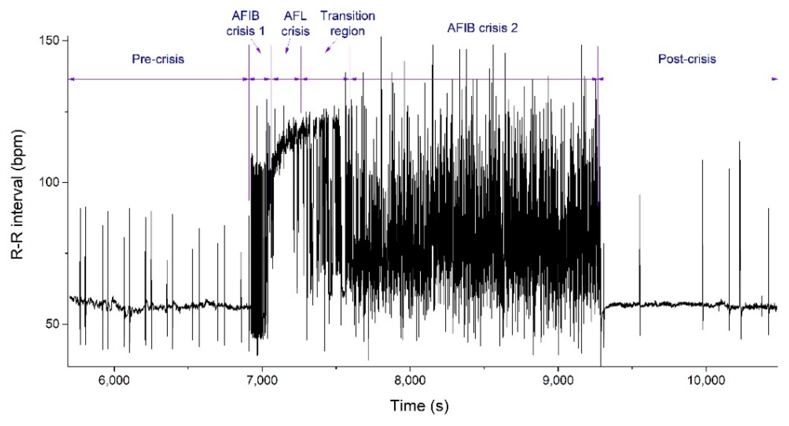
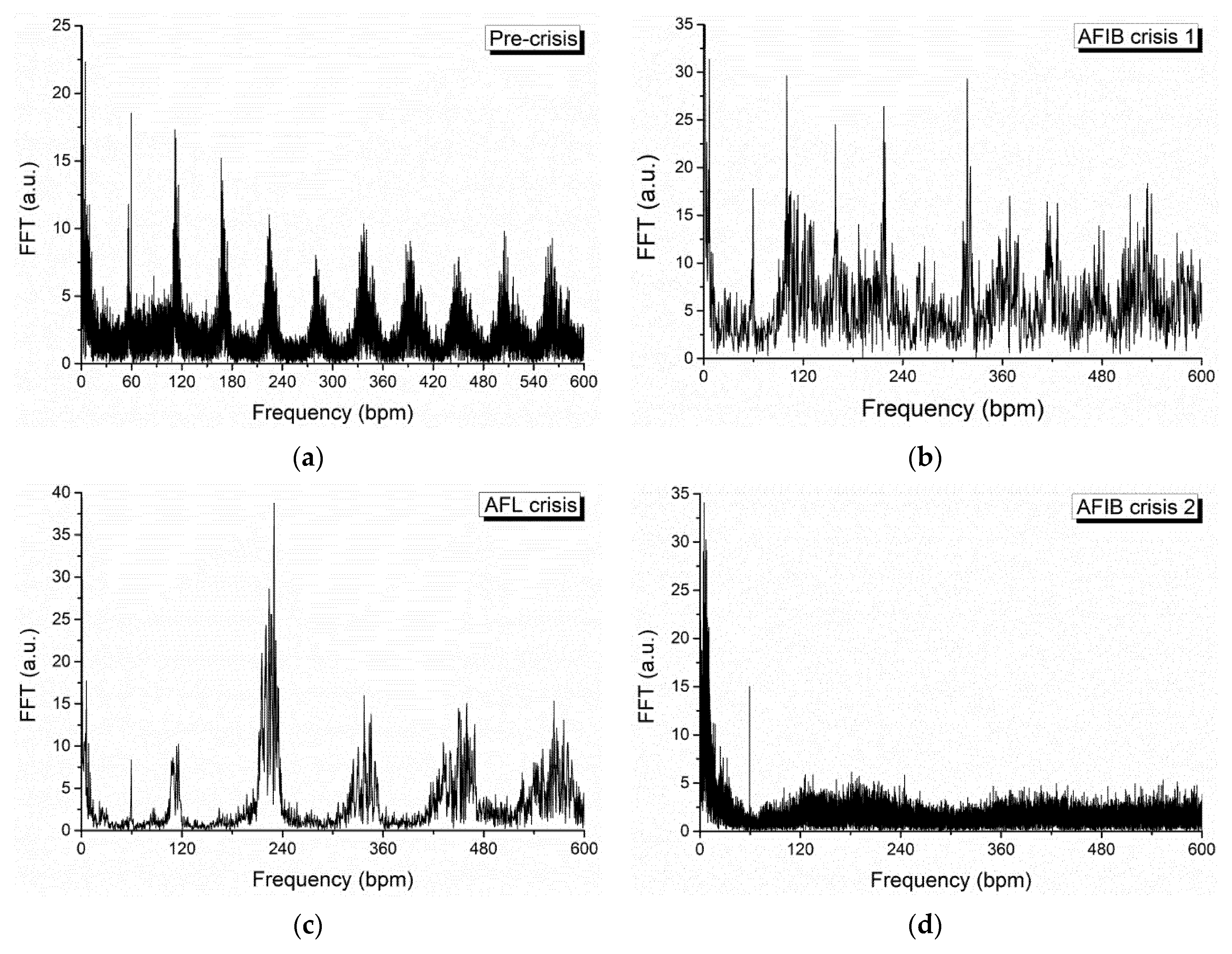
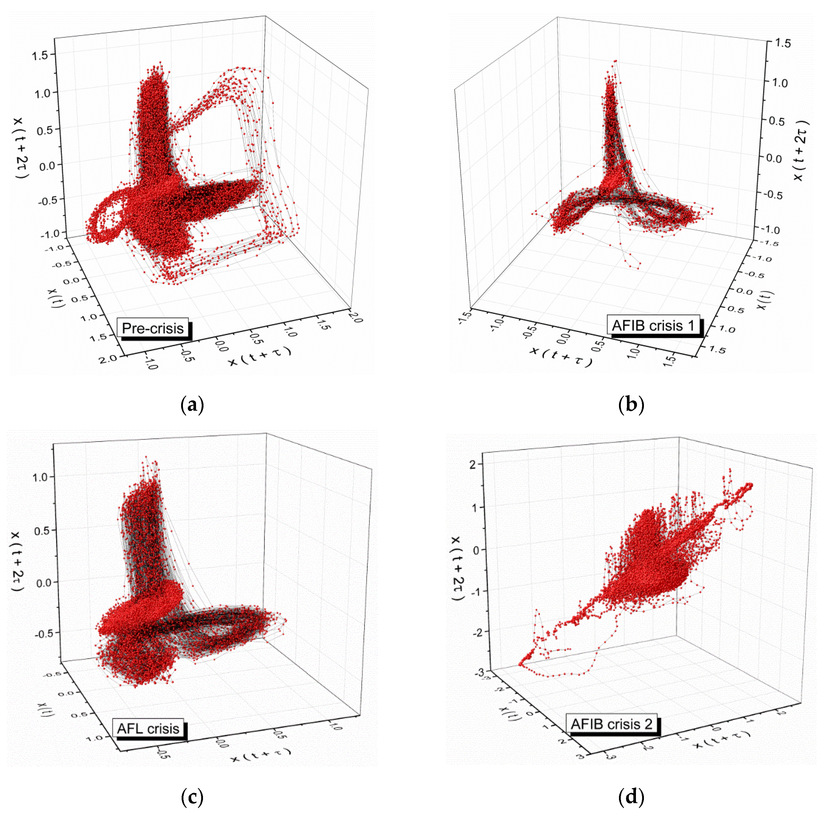
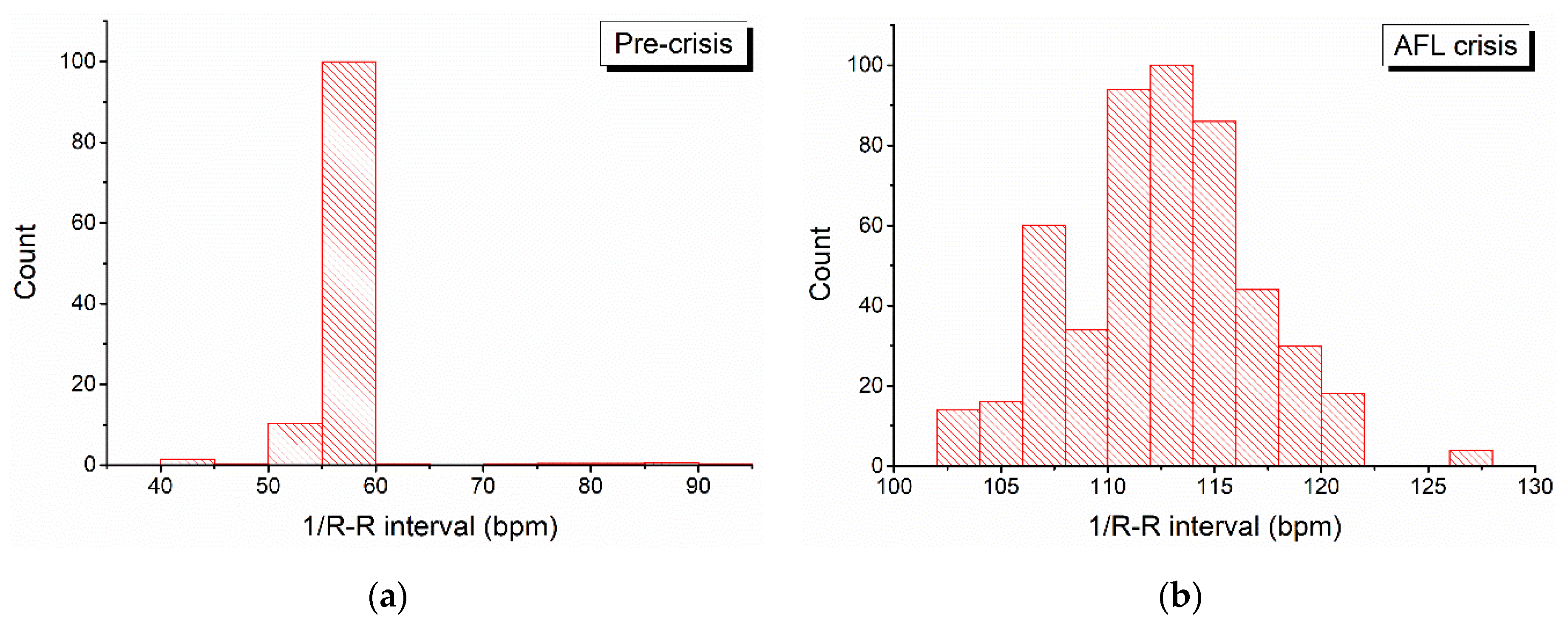
2. Analysis of Atrial Fibrillation by Applying Non-Linear Dynamics Methods

The analyzed electrocardiograms were downloaded from the PhysioNet database (PhysioNet). This allows all researchers to access a free collection of physiological signals (PhysioBank), recorded from a wide range of patients, as well as specialized software for viewing and analyzing them. It is supported by the National Institute of General Medical Science (NIGMS) and the National Institute of Biomedical Imaging and Bioengineering (NIBIB), and free access is made in accordance with ODC Public Domain Dedication and License v1.0. Existing resources are made available to stimulate current research in the domain of studying complex biomedical and physiological signals. The signal we analyzed has the following traits (10-h recording time, sampling time of 4 ms, sampling rate of 250 recordings/s. a total of 9,205,760 points, amplitude between −0.6 mV and 0.9 mV).

In Figure 1, the analysis of the 1/R-R interval, corresponding to a cardiac cycle, highlights these three crises, two atrial fibrillations and one flutter fibrillations is presented. The analysis contains all of EKG fragments (5 s duration) corresponding to pre-crisis, first AFIB (AFIB 1), AFL, second AFIB (AFIB 2), and post-crisis, respectively.

In Appendix A, details about the EKG signal fragments, referring to Figure 1, can be consulted.

In pre-crisis and post-crisis, the signals are normal. In the first AFIB, heart rate increases slowly, then it shows a rapid increase in AFL, slowly decreasing afterwards in the second AFIB. The first step in implementing a non-linear analysis concerns the number am amplitude several oscillation frequencies, which are known to be used for spotting various chaos transition scenarios. In Figure 2 we present the Fouriér specters for amplitudes of signals from Figure 1. The sudden appearance of AFIB crisis 1 (Figure 2b) leads to non-monotonous distribution of main oscillation frequencies and we see their number reduced from approximately 10 (pre-crisis) to 5 in the AFL (Figure 2c). The AFIB crisis 2 (Figure 2d) showcases all the signature of a chaotic signal with a quasi-infinite number of oscillations of similar amplitudes.

Figure 3 shows the systems dynamics attractors in the phase space reconstructed through the delay time method, determined using the auto-correlation function. It can be seen that a significant change is seen in the shape and structure of the attractor. For pre-crisis signals we observe 7 main regions which are not clearly defined, result induced by the abundance of frequencies around the main ones identified from FFT analysis. The AFB crisis 1 and AFL attractors are similar to a twisted Lorenz-type attractor with a strong center for high frequencies, thus offering a first identifiable feature in attractor analysis. Finally, we observe that in AFIB crisis 2 no distinguishable feature can be seen, with only abundance oscillation modes.

Results of Signal Analysis

We must highlight the clear difference between the geometry of attractors corresponding to the two atrial crises (AFIB 1 and 2), and also the differences between pre-crisis and post-crisis. This suggests a defibrillator was used to restore normal heart rhythm. Further histogram analysis of signals from Figure 1, presented in Figure 4, shows that, in the beginning, during the pre-crisis period, the pulse is stable around 60 bpm. It tends to increase during the first atrial fibrillation crisis, with a maximum of around 110 bpm. During flutter fibrillation, the pulse has values between 100–130 bpm. The histogram corresponding to the second atrial fibrillation has an approximately Gaussian distribution, with a maximum at 60–80 bpm. During post-crisis the pulse stabilizes, reaching 60 bpm.

The statistical analysis extended for all signals is summarized in

Table 1. Statistical values associated with heart rate variations (1/R-R interval).

Signal	1/R-R Interval Median (bpm)	Variance	Geometric Standard Deviation	Skewness	Kurtosis	Largest Lyapunov Exponent
Pre-crisis	56.3909	16.858	1.0673	4.4938	37.6779	0.013981
AFIB 1	53.3807	718.649	1.4309	0.7814	−1.098	0.211145
AFL	115.3846	17.9911	1.2105	−0.0359	0.462	0.082811
AFIB 2	76.9231	391.197	1.2662	0.7047	0.0456	0.138646
Post-crisis	56.6037	22.871	1.0684	8.2509	82.8455	0.014529

. Pulse average during the normal functioning of the heart is approximately 57 bpm. It increases up to over 69 bpm during AFIB 1, over 81 bpm during AFIB 2, and over 108 bpm during flutter. Regarding variation, a 40-time increase can be observed at the onset of AFIB 1, when compared to the normal functioning of the heart. The skewness and kurtosis values are in accordance with pulse rate distributions from histograms in Figure 4. The Lyapunov exponent has positive values, close to zero for normal heart rhythm, and with values over one order of magnitude higher in the case of fibrillation crises, highlighting a chaotic behavior for cardiac muscle dynamics. Nonlinear dynamics is nowadays widely employed in the study of biological phenomena. Taking into account that abnormal heart rhythms display chaotic behaviors, in our opinion, the specific attractor dynamics can constitute a method for evaluating various cardiac afflictions. By implementing mathematical procedures specific to nonlinear dynamics: constructing strange attractors, skewness, kurtosis, histograms, Lyapunov exponent, etc., a new method for evaluating atrial fibrillations was devised. This analysis as is presented in Figure 3, shows that their dynamics reflect abnormal heart rhythms following the evolution of the EKG signals. The skewness and kurtosis values are in accordance with pulse rate distributions from histograms of the analyzed signals. The Lyapunov exponent has positive values, close to zero for normal heart rhythm, and with values over one order of magnitude higher in the case of fibrillation crises, highlighting a chaotic behavior for cardiac muscle dynamics. In this conjecture, the dynamics of strange attractors generated in the phase space reflect abnormal heart rhythms. The presented results show that by applying nonlinear dynamics methods for analyzing the heart electrical activity we can obtain valuable information regarding fibrillation crises. Our method could be used for developing new models for medical diagnosis and evolution tracking of heart diseases, based on specific patterns.

3. The Reconstruction of EKG Signals through Scale Relativity Theory

Common models used to describe biological structure dynamics are based on a combination of basic theories derived especially from physics and computer simulations [14,15,16,17,18,19]. As such, the description of biological structure dynamics implies both computational simulations based on specific algorithms [17,20,21], as well as developments on usual theories of biophysics, concerning various classes of models. One class of models was developed on spaces with integer dimensions, i.e., a differentiable class of models (differentiable biophysical models) [14,15,16]. Another class of models has been developed on spaces with non-integer dimensions and has been explicitly written through fractional derivatives, i.e., a non-differentiable class of models (fractal or multifractal biophysical models) [20,21].

On the same considerations, linked with the previously mentioned models, a new class of biophysical models has arisen, based on Scale Relativity Theory, either in the monofractal dynamics as in the case of Nottale [22], or in the multifractal dynamics as in the case of the multifractal theory of motion [23]. Both in the context of [22], as well as in the one of [23], supposing that any biological structure dynamics are assimilated both structurally and functionally to a multifractal object, said dynamics can be described through motions of the biological system’s structural units, dependent on the chosen scale resolution, on continuous and non-differentiable curves (multifractal curves). Since for a large temporal scale resolution with respect to the inverse of the highest Lyapunov exponent [24,25], the deterministic trajectories of any structural units belonging to the biological system can be replaced by a collection of potential (“virtual”) trajectories, the concept of definite trajectory can be substituted by the one of probability density.

With all of the above considerations taken into account, in the description of the dynamics of any biological structure, the multifractality expressed through stochasticity becomes operational. Therefore, when describing such dynamics, it will be necessary to use multifractal functions (functions that are both time-space coordinates and scale resolution dependent) [22,23].

In the present section, it is shown that, by applying scale relativity theory, in its various forms, it is possible to reconstruct any type of EKG signal by means of harmonic mappings from the usual space to the hyperbolic one.

3.1. Dynamics through Markovian and Non-Markovian Fractalization Types at Various Scale Resolutions

Assuming that any biological system can be assimilated to a multifractal object, its dynamics in the multifractal Theory of Motion are described through continuous but non-differentiable curves (multifractal curves). Such an assumption has important consequences [22,23]:

(i)

The lengths of multifractal curves tend to infinity when the scale resolution $\delta t$ tends to zero (according to the Lebesgue Theorem [22]). Therefore, the space of such dynamics becomes a multifractal in the Mandelbrot sense [26].

(ii)

During the zoom operation of $\delta t$, any dynamics are related to the behaviors of a set of functions through the substitution principle $\delta t\equiv dt$.

(iii)

Any dynamics are described by multifractal functions. Then, two derivatives can be defined:

$$\begin{array}{l}\frac{d{Q}_{+}}{dt}=\underset{\Delta t\to 0}{\lim }\frac{Q\left(t,t+\Delta t\right)-Q\left(t,\Delta t\right)}{\Delta t},\\ \frac{d{Q}_{-}}{dt}=\underset{\Delta t\to 0}{\lim }\frac{Q\left(t,\Delta t\right)-Q\left(t-\Delta t,\Delta t\right)}{\Delta t}.\end{array}$$

(1)

The sign “$+$” specifies the forward dynamics. The sign “$-$” specifies the backward ones.

(iv)

The differential of the spatial coordinate has the form:

$$d_{\pm }{X}^i\left(t, dt\right)=d_{\pm }{x}^i\left(t\right)+d_{\pm }\xi \left(t, dt\right)$$

(2)

The differentiable part $d_{\pm }{x}^i\left(t\right)$ does not depend on the scale resolution, while the non-differentiable part $d_{\pm }\xi \left(t, dt\right)$ is scale resolution dependent.

(v)

The quantities $d_{\pm }\xi \left(t, dt\right)$ satisfy the relation:

$$d_{\pm }{\xi }^i\left(t, dt\right)={\lambda }_{\pm }^i{\left(dt\right)}^{\left[\frac{2}{f\left(\alpha \right)}\right]-1}, f\left(\alpha \right)=f\left[\alpha \left(D_F\right)\right]$$

(3)

where ${\lambda }_{\pm }^i\left(dt\right)$ are constant coefficients associated to differential-non-differential transition, $f\left[\alpha \left(D_F\right)\right]$ is the singularity spectrum of order α, α is the singularity index and D_F is the fractal dimension of the “motion curves.”

There are many modes of defining the fractal dimension. Thus, several fractal dimensions may be employed, but the fractal dimension in the sense of Hausdorff–Besikovitch [26] or the fractal dimension in the sense of Kolmogorov, are the most commonly used ones. In the case of many models, selecting one of these definitions and operating it in the context of any biological system dynamics implies that the value of the fractal dimension must be constant and arbitrary for the entirety of the dynamical analysis: for example, it is regularly found that D_F < 2 for correlative processes in the dynamics of any biological system, D_F > 2 for non-correlative processes. In the description of biological system dynamics we operate with $f\left[\alpha \left(D_F\right)\right]$ (i.e., simultaneously operating with several fractal dimensions, on multifractal manifolds, as in the multifractal theory of motion) instead of operating with D_F (i.e., with a single fractal dimension, on monofractal manifolds, as in the case of Nottale’s model). This leads to a series of advantages [13], such as the possibility to identify the areas of biological system dynamics that are characterized by a certain fractal dimension (for example, cell dynamics from either normal or tumoral tissues) or to identify the number of areas in the biological system dynamics for which the fractal dimensions are situated in an interval of values (for example, cell dynamics from tissue with various metastasis degrees). Finally, one of the biggest advantages of the method is the ability to identify classes of universality in the biological system dynamics, even when regular or strange attractors have various aspects (for example, the diagnosis of diseases from regular or strange attractor dynamics, as shown here).

(vi)

The differential time reflection invariance is recovered by means of the operator:

$$\frac{\widehat{d}}{dt}=\frac{1}{2}\left(\frac{d_{+}+d_{-}}{dt}\right)-\frac{i}{2}\left(\frac{d_{+}-d_{-}}{dt}\right).$$

(4)

In such context, applying this operator to $X^i$, yields the complex velocity:

$${\widehat{V}}^i=\frac{\widehat{d}{X}^i}{dt}=V_D^i-V_F^i$$

(5)

with

$$V_D^i=\frac{1}{2}\frac{d_{+}{X}^i+d_{-}{X}^i}{dt},V_F^i=\frac{1}{2}\frac{d_{+}{X}^i-d_{-}{X}^i}{dt},i=1,2,3.$$

(6)

In this relation the differential velocity $V_D^i$ is scale resolution independent, while the non–differentiable one $V_F^i$ is scale resolution dependent.

(vii)

Since the multi-fractalization describing biological structures dynamics implies stochasticization, the whole statistic “arsenal” (averages, variances, covariances, etc.) are operational. Thus, for example, let us select the subsequent functionality:

$$\langle d_{\pm }{X}^i\rangle \equiv d_{\pm }{x}^i,$$

(7)

with

$$\langle d_{\pm }{\xi }^i\rangle =0.$$

(8)

(viii)

The biological structures dynamics, with previous functionality, can be described through the scale covariant derivative given by the operator

$$\frac{\widehat{d}}{dt}={\partial }_t+{\widehat{V}}^i{\partial }_i+D^{lk}{\partial }_l{\partial }_k,$$

(9)

where

$${\mathrm{D}}^{\mathrm{lp}}=\frac{1}{4}{\left(\mathrm{dt}\right)}^{\frac{2}{\mathrm{f}\left(\mathsf{\alpha }\right)}-1}\left({\mathrm{d}}^{\mathrm{lp}}+{\mathrm{i} \overline{\mathrm{d}}}^{\mathrm{lp}}\right), \mathrm{i}=\sqrt{-1}$$

(10)

$${\mathrm{d}}^{\mathrm{lp}}={\mathsf{\lambda }}_{+}^{\mathrm{l}}{\mathsf{\lambda }}_{+}^{\mathrm{p}}-{\mathsf{\lambda }}_{-}^{\mathrm{l}}{\mathsf{\lambda }}_{-}^{\mathrm{p}}$$

(11)

$${\overline{\mathrm{d}}}^{\mathrm{lp}}={\mathsf{\lambda }}_{+}^{\mathrm{l}}{\mathsf{\lambda }}_{+}^{\mathrm{p}}-{\mathsf{\lambda }}_{-}^{\mathrm{l}}{\mathsf{\lambda }}_{-}^{\mathrm{p}}$$

(12)

$${\partial }_{\mathrm{t}}=\frac{\partial }{{\partial }_{\mathrm{t}}},{\partial }_{\mathrm{l}}=\frac{\partial }{\partial {\mathrm{X}}^{\mathrm{l}}},{\partial }_{\mathrm{l}}{\partial }_{\mathrm{p}}=\frac{\partial }{\partial {\mathrm{X}}^{\mathrm{l}}}\frac{\partial }{\partial {\mathrm{X}}^{\mathrm{p}}},\mathrm{l}, \mathrm{p}=1, 2, 3$$

(13)

Now, accepting the scale covariant principle in the describing of any biological structure dynamics, the conservation law of the specific momentum (i.e., geodesic equations on a multifractal manifold) takes the form:

$$\frac{{\hat{\mathrm{d}}\hat{\mathrm{V}}}^{\mathrm{i}}}{\mathrm{dt}}={\partial }_{\mathrm{t}}{\hat{\mathrm{V}}}^{\mathrm{i}}+{\hat{\mathrm{V}}}^{\mathrm{l}}{\partial }_{\mathrm{i}}{\hat{\mathrm{V}}}^{\mathrm{i}}+\frac{1}{4}{\left(\mathrm{dt}\right)}^{\left[\raisebox{1ex}{$2$}\!\left/ \!\raisebox{-1ex}{$\mathrm{f}\left(\mathsf{\alpha }\right)$}\right.\right]-1}{\mathrm{D}}^{\mathrm{lp}}{\partial }_{\mathrm{l}}{\partial }_{\mathrm{p}}{\hat{\mathrm{V}}}^{\mathrm{i}}=0$$

(14)

The explicit form of $D^{lp}$ depends on the type of multi-fractalization used. It can be admitted that the multi-fractalization process can take place through various stochastic processes. Stochastic dynamics can be Markovian (thus, memoryless) biological processes. This is the case of scale relativity theory in Nottale’s sense, referring to biological dynamics on monofractal manifolds (with fractal dimension $D_F=2$). For non-Markovian biological processes, memory-like qualities are expected. Since biological processes usually display some sort of memory-related traits, it is then necessary to operate with mathematical procedures vastly different than the ones previously mentioned. In this case, wherein it is possible to generalize many of the previous results [21,23], the following constraints are admitted:

$$\frac{1}{4}{\left(\mathrm{dt}\right)}^{\left[\raisebox{1ex}{$2$}\!\left/ \!\raisebox{-1ex}{$\mathrm{f}\left(\mathsf{\alpha }\right)$}\right.\right]-1}{\mathrm{d}}^{\mathrm{lp}}={\mathsf{\alpha }\mathsf{\delta }}^{\mathrm{lp}},\hspace{1em}\frac{1}{4}{\left(\mathrm{dt}\right)}^{\left[\raisebox{1ex}{$2$}\!\left/ \!\raisebox{-1ex}{$\mathrm{f}\left(\mathsf{\alpha }\right)$}\right.\right]-1}{\overline{\mathrm{d}}}^{\mathrm{lp}}={\mathsf{\beta }\mathsf{\delta }}^{\mathrm{lp}}$$

(15)

where $\alpha$ and $\beta$ are two constant coefficients associated to the differential-nondifferential scale transition, and ${\delta }^{lp}$ is Kronecker’s pseudotensor. In such context, the conservation laws on multifractal and Euclidian manifolds are given in Appendix B, while in Appendix C nonlinear behaviors at non-differentiable scale are presented.

3.2. Dynamics Generated by Differential Geometry of Riemann Type in Scale Space

The constraints in Equation (15), through which multi-fractalization by means of stochasticization of non-Markovian type is explained, imply the determination of eigenvalues of two $3\times 3$ matrices (let them be $d^{lp}$ and ${\overline{d}}^{lp}$), which formally lead to the cubic equation in binomial form:

$$a_0{x}^3+3a_1{x}^2+3a_{2}x+a_3=0$$

(16)

where the coefficients $a_i$ are real (with $i=0,1,2,3$).

Now, it is possible to associate a Riemann space to the family of cubics in Equation (16), as it will be seen. The basis of approach is the fact that the simple transitive group with real parameters [27]:

$$x_k\leftrightarrow \frac{a{x}_k+b}{c{x}_k+d},a, b, c ϵ R$$

where $x_k$ are the roots of the cubic in Equation (16), in the form:

$$x_1=\frac{h+h^{*}·k}{1+k},x_2=\frac{h+\epsilon ·h^{*}·k}{1+\epsilon ·k},x_3=\frac{h+{\epsilon }^2·h^{*}·k}{1+{\epsilon }^2·k}$$

(17)

with h, h^*—the roots of Hessian

$$\left(a_0{a}_2-a_1^2\right)x^2+\left(a_0{a}_3-a_1{a}_2\right)x+\left(a_1{a}_3-a_2^2\right)=0$$

(18)

and ε ≡ (−1 + i√3)/2 the cubic root of unity (i ≡ √(−1)), induces a simply transitive group for the quantities h, h^* and k, whose action is:

$$h\leftrightarrow \frac{ah+b}{ch+d},h^{*}\leftrightarrow \frac{a{h}^{*}+b}{c{h}^{*}+d},k\leftrightarrow \frac{c{h}^{*}+d}{ch+d}·k$$

(19)

The structure of this group is typical of a SL(2, R) one, which we take in the standard form

$$\left[B_1,B_2\right]=B_1,\left[B_2,B_3\right]=B_3,\left[B_3,B_1\right]=-2B_2$$

(20)

where B_k are the infinitesimal generators of the group. Because the group is simply transitive, these generators can be found as the components of the Cartan frame [28,29] from the relation

$$\begin{array}{ll}d\left(f\right)& ={\displaystyle \sum }\frac{\partial f}{\partial x^k}d{x}^k\\ & =\left[{\omega }^1\right(h^2\frac{\partial }{\partial h}+h^{*2}\frac{\partial }{\partial h^{*}}\\ & +\left(h-h^{*}\right)k\frac{\partial }{\partial k})+2{\omega }^2\left(h\frac{\partial }{\partial h}+h^{*}\frac{\partial }{\partial \overline{h}}\right)\\ & +{\omega }^3\left(\frac{\partial }{\partial h}+\frac{\partial }{\partial h^{*}}\right)]\left(f\right)\end{array}$$

(21)

where ω^k are the components of the Cartan coframe to be found from the system

$$\begin{array}{c}dh={\omega }^1{h}^2+2{\omega }^{2}h+{\omega }^3\\ d{h}^{*}={\omega }^1{h}^{*2}+2{\omega }^2{h}^{*}+{\omega }^3\\ dk={\omega }^{1}k\left(h-h^{*}\right)\end{array}$$

Thus, both the infinitesimal generators and the coframe are obtained, by identifying the right hand side of Equation (21) with the standard dot product of SL(2, R) algebra:

$${\omega }^1{B}_3+{\omega }^3{B}_1-2{\omega }^2{B}_2$$

so that

$$\begin{array}{c}{B}_1=\frac{\partial }{\partial h}+\frac{\partial }{\partial h^{*}},\\ B_2=h\frac{\partial }{\partial h}+h^{*}\frac{\partial }{\partial h^{*}}\\ B_3=h^2\frac{\partial }{\partial h}+h^{*2}\frac{\partial }{\partial h^{*}}+\left(h-h^{*}\right)k\frac{\partial }{\partial k}\end{array}$$

(22)

and

$$\begin{array}{c}{\omega }^1=\frac{dk}{\left(h-h^{*}\right)k},2{\omega }^2=\frac{dh-d{h}^{*}}{h-h^{*}}-\frac{h+h^{*}}{h-h^{*}}\frac{dk}{k}\\ {\omega }^3=\frac{hd{h}^{*}-h^{*}dh}{h-h^{*}}+\frac{h{h}^{*}}{h-h^{*}}\frac{dk}{k}\end{array}$$

In real terms,

$$h=u+iv, k=e^{i\varphi }$$

these last equations can be written as

$$\begin{array}{c}{B}_1=\frac{\partial }{\partial u},B_2=u\frac{\partial }{\partial u}+v\frac{\partial }{\partial v},B_3=\left(u^2-v^2\right)\frac{\partial }{\partial u}+2uv\frac{\partial }{\partial v}+2v\frac{\partial }{\partial \varphi }\\ {\omega }^1=\frac{\partial \varphi }{2v},{\omega }^2=\frac{dv}{v}-\frac{u}{v}\partial \varphi ,{\omega }^3=\frac{u^2+v^2}{2v}\partial \varphi +\frac{vdu-udv}{v}\end{array}$$

(23)

Mention should be made that it is also possible to work with the absolute invariant differentials [27]

$${\omega }^1=\frac{dh}{\left(h-h^{*}\right)k},{\omega }^2=-i\left(\frac{dk}{k}-\frac{dh+d{h}^{*}}{h-h^{*}}\right),{\omega }^3=-\frac{kd{h}^{*}}{h-h^{*}}$$

(24)

or, in real terms, exhibiting a three-dimensional Lorentz structure of this space

$$\begin{array}{c}{\mathsf{\Omega }}^1\equiv {\omega }^2=d\varphi +\frac{du}{v}\\ {\mathsf{\Omega }}^2=\cos \varphi \frac{du}{v}+\sin \varphi \frac{dv}{v}\\ {\mathsf{\Omega }}^3=-\sin \varphi \frac{du}{v}+\cos \varphi \frac{dv}{v}\end{array}$$

(25)

This representation highlights the connection with the Poincaré depiction of the Lobachevsky plane. Indeed, the metric here is

$$d{s}^2=-{({\mathsf{\Omega }}^1)}^2+{({\mathsf{\Omega }}^2)}^2+{({\mathsf{\Omega }}^3)}^2=-{\left(d\varphi +\frac{du}{v}\right)}^2+\frac{{\left(du\right)}^2+{\left(dv\right)}^2}{v^2}$$

(26)

Let it be noted that, when Ω¹ = 0, (26) is reduced to the Poincaré metric. Through this restriction, $\varphi$ becomes the angle of parallelism of the hyperbolic plane, i.e., the connection [30,31].

Taking into account the previous aspects, important correlations with the geometry of Lobachevsky can be established, by the meaning of the condition Ω¹ = 0 for any family of cubic equations of type in Equation (16). It turns out that it expresses the so-called apolar transport of cubics [27]. This transport is defined by the condition that any root of the “transported” cubic is in a harmonic relation with any root of the “original” cubic, with respect to the other two remaining roots of the original cubic:

$$\frac{y_1-x_j}{y_1-x_k}:\frac{x_i-x_j}{x_i-x_k}=-1;i\ne j\ne k\ne i$$

(27)

In all positive permutations of the indices I, j, k and for every l. Therefore, each new root ($y_1$) and each of the corresponding old ones ($x_i$), are in harmonic range with respect to the other two old roots ($x_i$, $x_k$). Then it can be proved that the conditions from Equation (27) boil down to the vanishing of the bilinear invariant of the two cubics, analogous to the bilinear invariant of the quadratics:

$$a_3{b}_0-3a_2{b}_1+3a_1{b}_2-a_0{b}_3$$

(28)

Here a_m denote the coefficients of the original cubic, while b_m denotes the coefficients of the transported cubic. Obviously, this invariant is analogous to the one from the case of two quadratics, whose vanishing expresses the fact that their roots are in harmonic sequence. The geometry related to this invariant is a century old [32], and Dan Barbilian seemed particularly fond of it [33], for he elaborated for a long while on its different aspects, especially related to the geometry of the triangle. As the triangle comes nowadays in relation with the construction of skyrmions from instantons [34], from a point of view closely related to its geometry, it is therefore worth considering this connection, which turns out to be strictly related to the physics of continua. Let it be noted that, in discrete spaces (i.e., network space), phenomena of such triangles can also be observed [35].

Now, if the two cubics are infinitesimally close, then the condition of their transport by involution reduces to

$$a_{3}d{a}_0-3a_{2}d{a}_1+3a_{1}d{a}_2-a_{0}d{a}_3=0$$

(29)

Using here the relation

$$\begin{array}{c}{a}_0=1+k^3\\ a_1=-\left(h+h^{*}·k^3\right)\\ a_2=h^2+h^{*2}·k^3\\ a_3=-\left(h^3+h^{*3}·k^3\right)\end{array}$$

(30)

for the coefficients, the condition of apolar transport of the cubics amounts to

$$-{(h-h^{*})}^3{k}^3\left(\frac{dk}{k}-\frac{dh+d{h}^{*}}{h-h^{*}}\right)=0$$

(31)

As the cubics are asumed to have distinct roots, this condition is satisfied if, and only if, the differential form Ω¹ is null. Therefore, the parallel transport of the hyperbolic plane actually represents the apolar transport of the cubics.

Now, accepting the contraint in Equation (31), the metric in Equation (26) becomes reducible to one belonging to the hyperbolic space:

$$d{s}^2=-\frac{dhd{h}^{*}}{{\left(h-h^{*}\right)}^2}=\frac{{\left(du\right)}^2+{\left(dv\right)}^2}{v^2}$$

(32)

Then, according to [23,27], harmonic mappings from the usual space to the hyperbolic plane can be described through the stationary values of the Lagrangean:

$$L=-4\frac{\nabla h\nabla \overline{h}}{{\left(h-\overline{h}\right)}^2}$$

(33)

specific to the variational problems:

$$\delta {\displaystyle \int }Ld\mathrm{v}=0$$

(34)

where $\nabla$ corresponds to the gradient and $d\mathrm{v}$ corresponds to the infinitesimal volume. In such a context, the field equations result:

$$\left(h-\overline{h}\right)\nabla \left(\nabla h\right)=2{\left(\nabla h\right)}^2$$

(35)

Of course, along with Equation (35), the field equations for the complex conjugate $\overline{h}$ are also satisfied.

The solution of Equation (35) has the form:

$$h=i\frac{\cosh \chi -\sinh \chi e^{-i\overline{\mathsf{\Omega }}}}{\cosh \chi +\sinh \chi e^{-i\overline{\mathsf{\Omega }}}}$$

(36)

This relation will be used in what follows, for the reconstruction of any type of EKG signal, which appears in the dynamics concerning atrial fibrillation. A comparative presentation of the reconstructed EKG and empirical signals is shown in Figure 5. It is important to note here that the fractal model, as per its generalist scope cannot emulate the shape of the EKG signal. However, at its core, the model considers two oscillations with different oscillations. The modulation of the signal is done by changing the fractality degree. The increase of the fractalization degree and thus of the maximum scale for the harmonic mapping of the system leads to the increase in frequency depicting well the increase see in AFIB crisis 1. Further the slight modulation of the signal coupled with a decrease in the oscillation amplitude similar to the AFL crisis part where we do see an uncorrelated modulation of the high-frequency oscillations. The AFIB crisis 2 is seen reflected by the model with a high frequency and a chaos-like behavior. The fluctuation in the amplitude of the signal is also captured by the model. It is important to note there that multifractal system built here, although it reaches a quasi-chaotic regime, it does not remain in that state. The subsequent change in fractality degree will lead to a sudden transition into the regular oscillatory regime as seen for ω = 6 (equivalent to a pre-crisis state), this feature is also seen empirically in Figure 1 where we see sudden transitions into crisis and post-crisis states.

4. Conclusions

The main conclusions of this paper are the following:

(i)

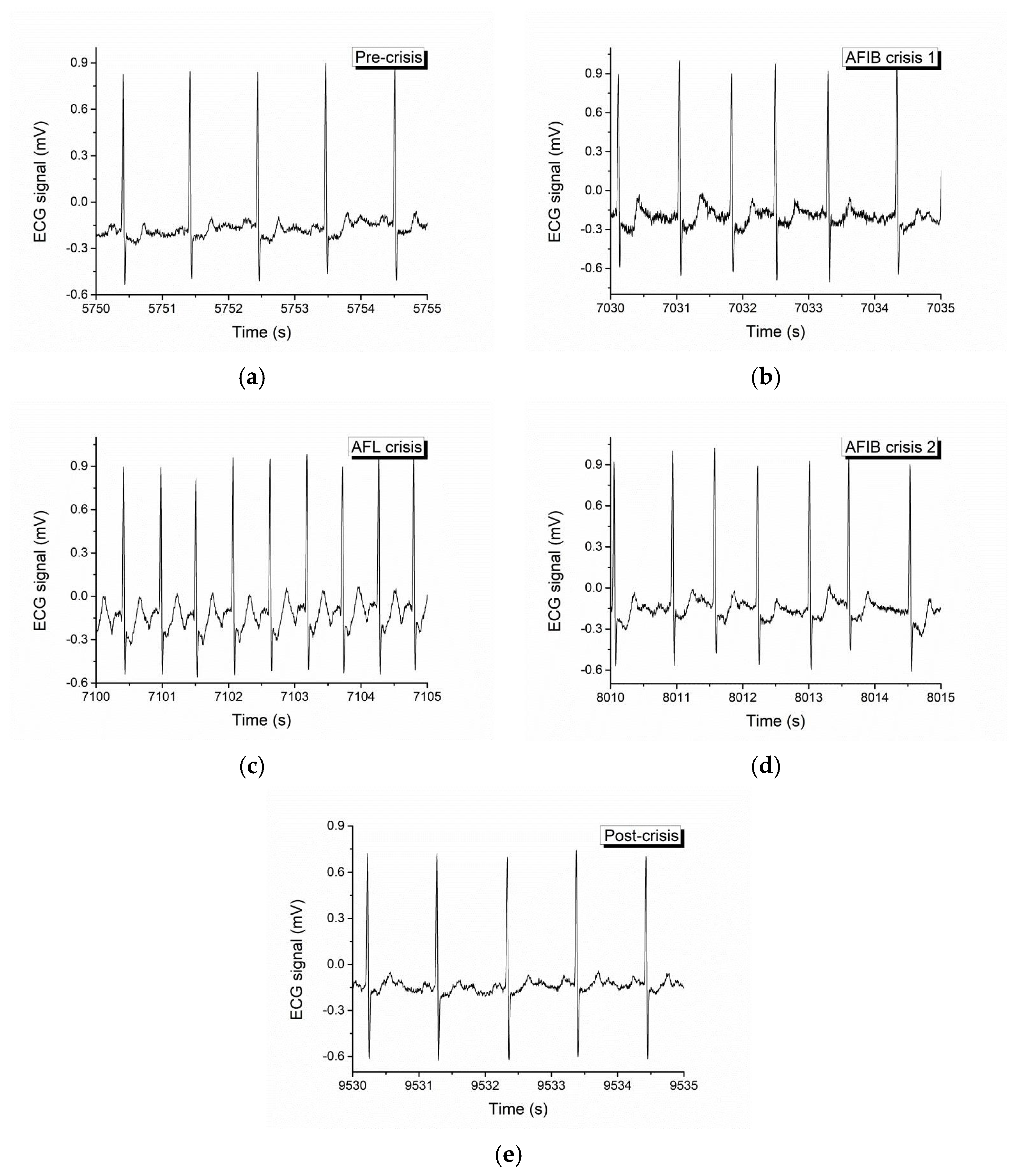
Diagnostics and evolution of atrial fibrillation by applying non-linear dynamics method skewness and kurtosis values are in accordance with pulse rate distributions from the histograms of the analyzed ECG signal. The Lyapunov exponent has positive values, close to zero for normal heart rhythm, and with values over one order of magnitude higher in the case of fibrillation crises, highlighting a chaotic behavior for cardiac muscle dynamics. Additionally, in the case of atrial flutter, a pattern of alternating 2:1, 3:1, 4:1, and 5:1 conduction ratio can be observed. Some abnormal heart rhythms were analyzed through strange attractors dynamics in the reconstructed phase space. For each stage of a crisis, a specific strange attractor was associated, proving that the specific attractors dynamics can constitute a valid method for evaluating various cardiac afflictions. The obtained results encourage us to further pursue this line of research.

(ii)

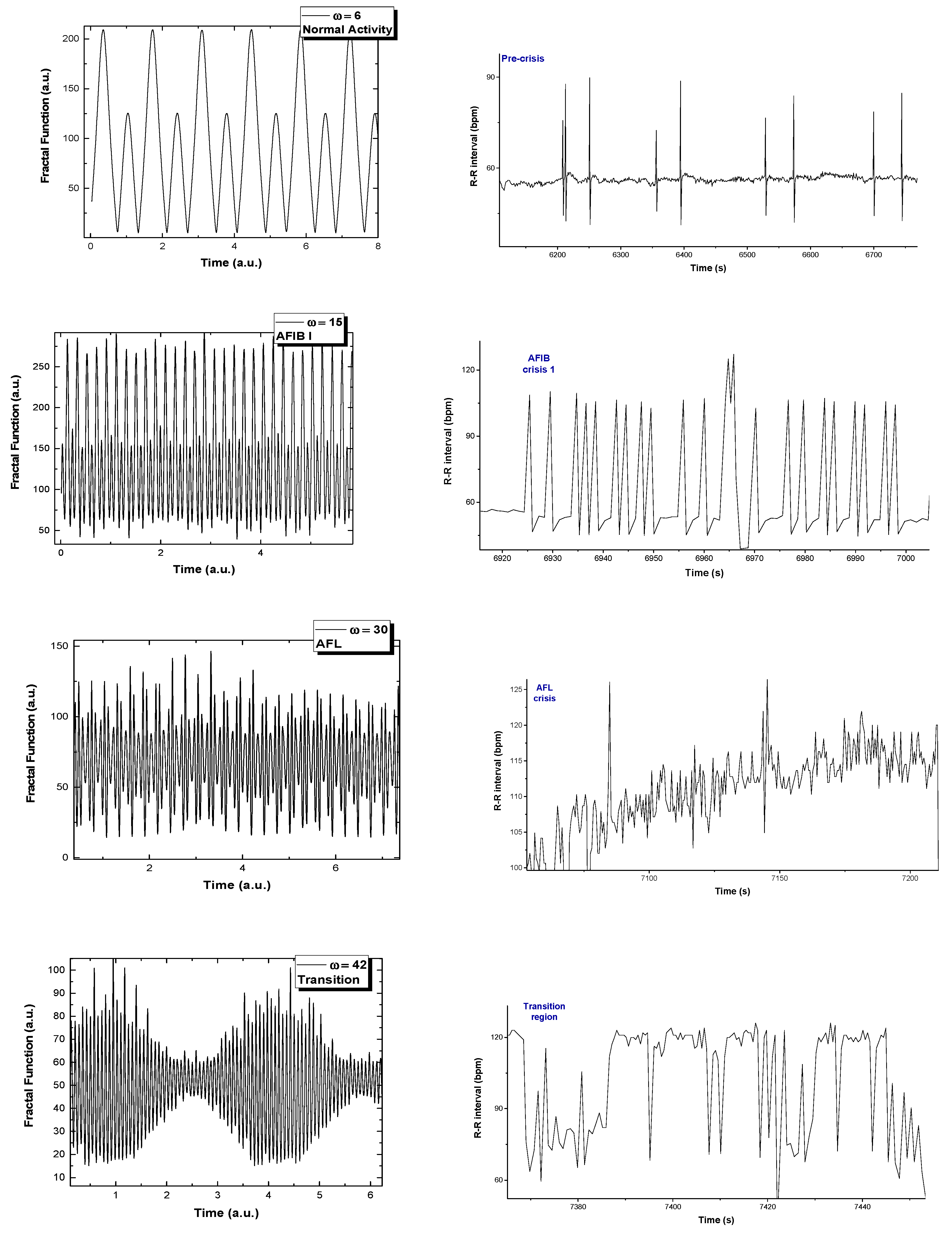
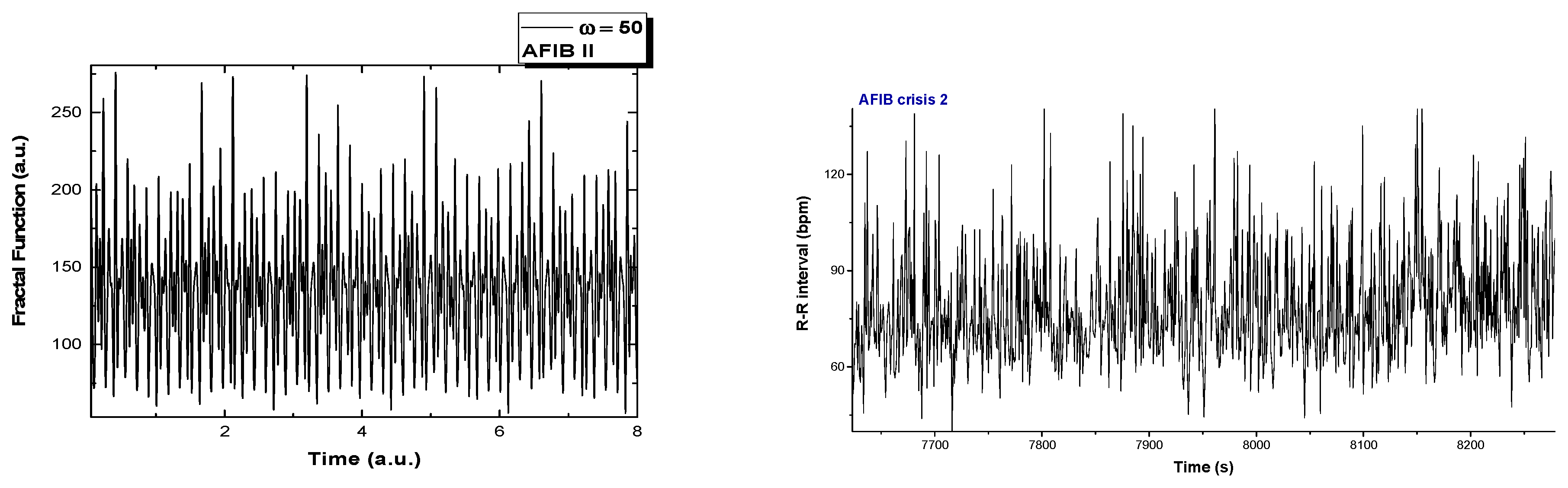
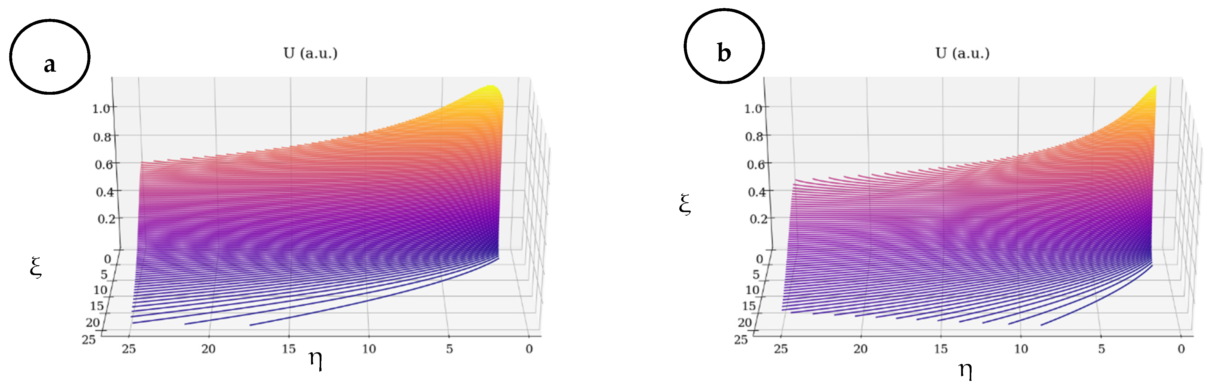
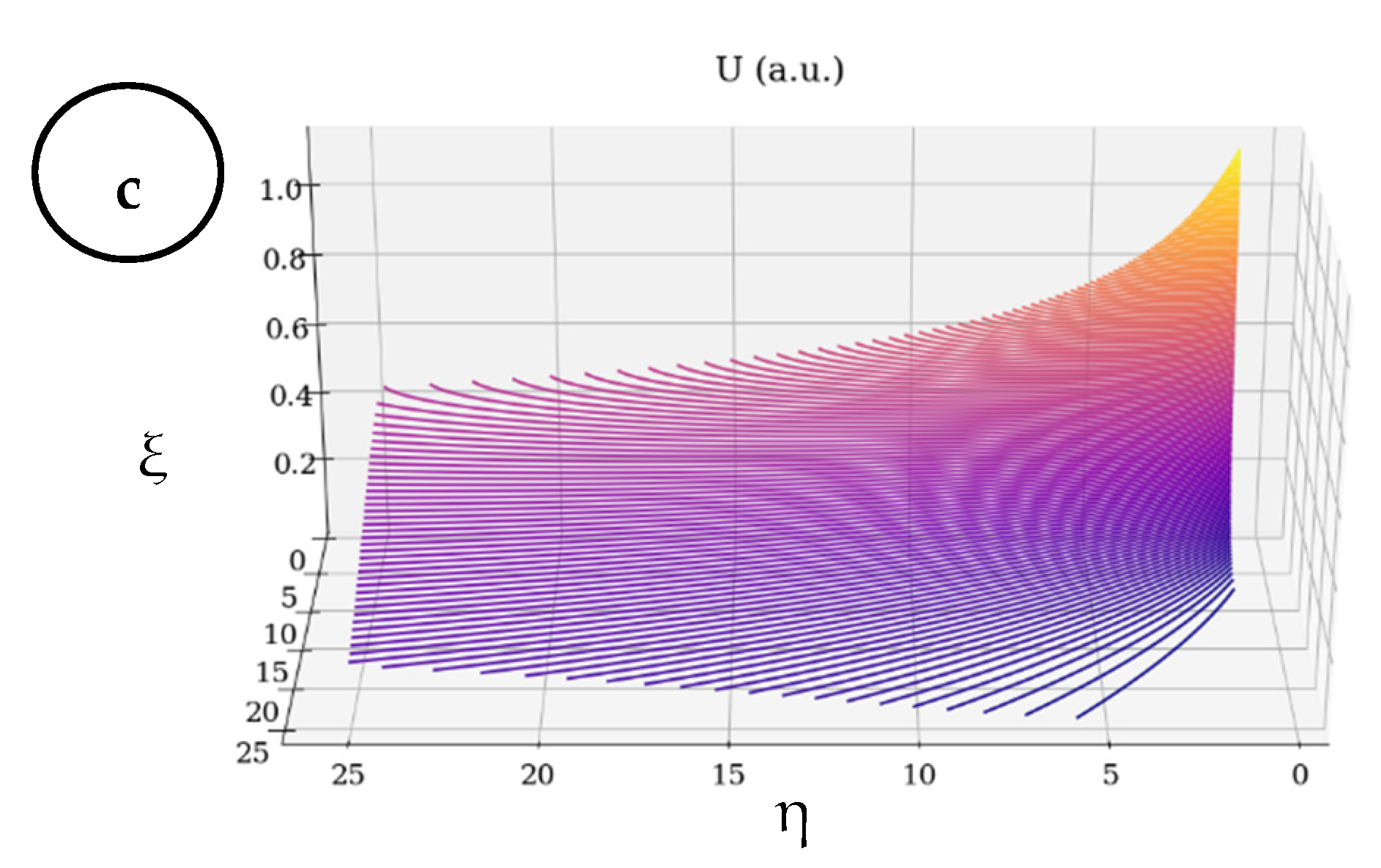
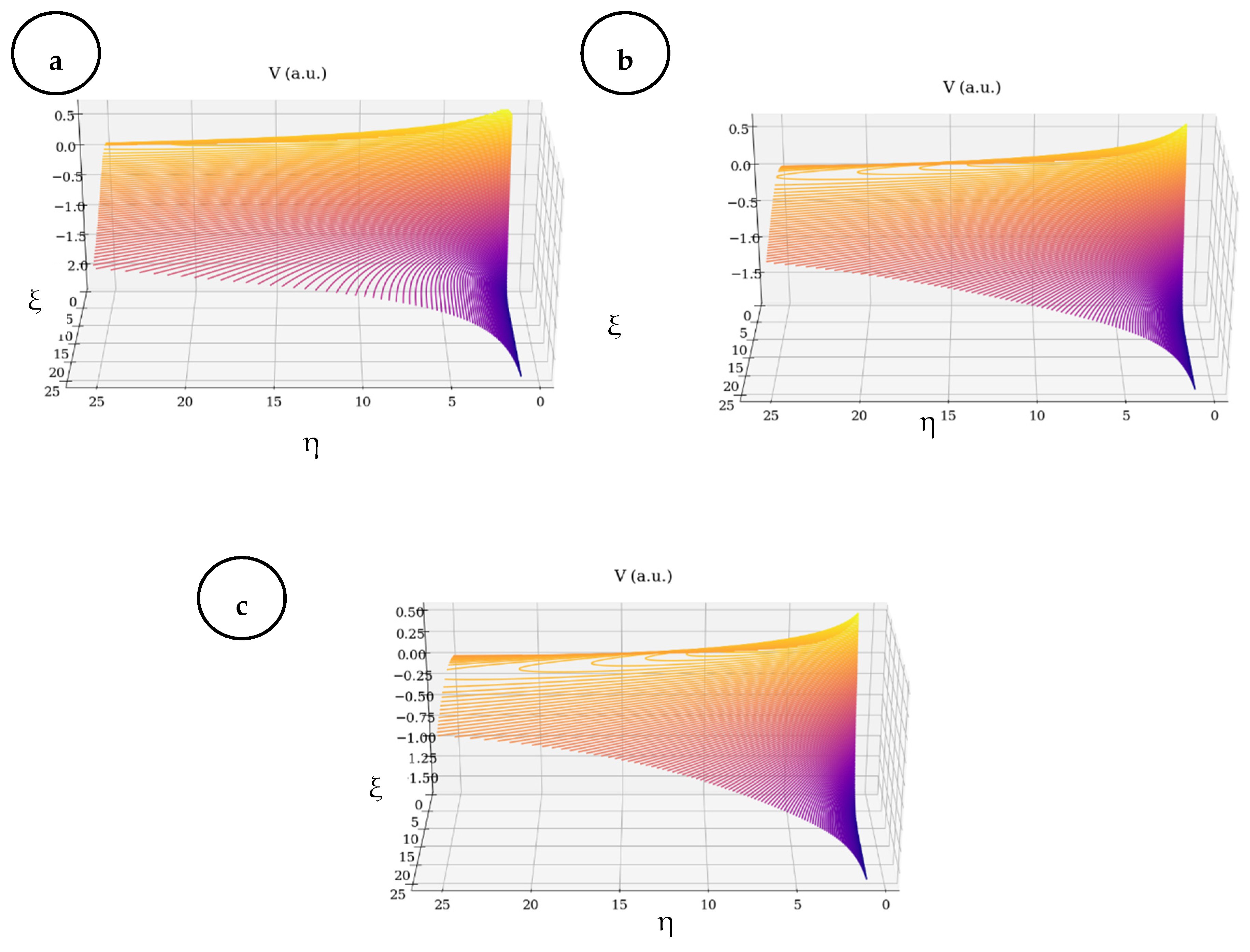
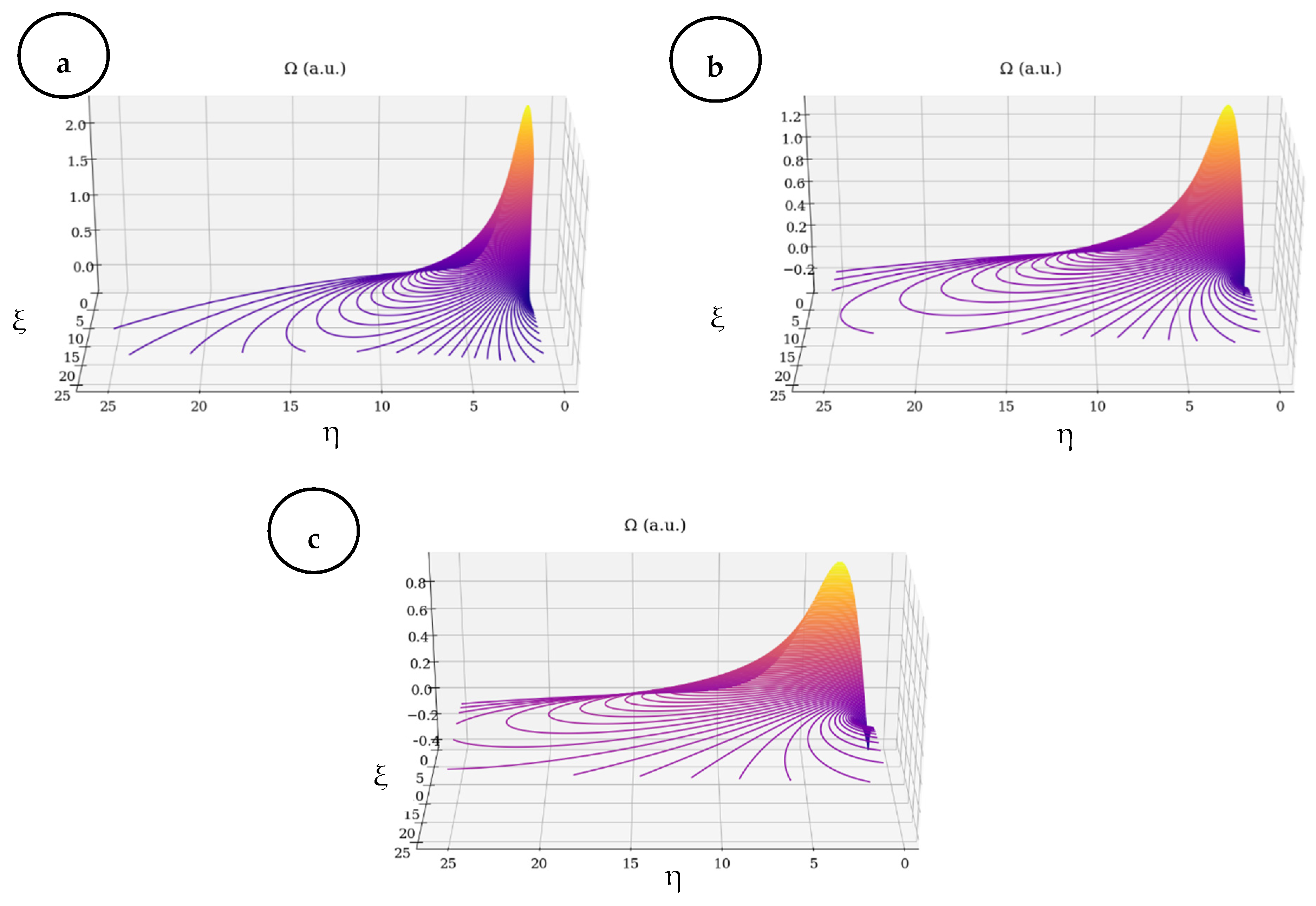
Based on multi-fractalization through Markovian and non-Markovian-type stochasticizations in the framework of the scale relativity theory, any type of EKG signal can be reconstructed by means of harmonic mappings from the usual space to the hyperbolic one. These mappings mime various scale transitions by differential geometries, with parallel transport of direction in Levi–Civita sense, in Riemann-type spaces. The aforementioned spaces are associated to families of cubics, with symmetries of SL(2R)-type (i.e., invariances with respect to SL(2R)-type transformations).

(iii)

Then, the two operational procedures are not mutually exclusive, but rather become complementary, through their finality regarding the obtainment of valuable information concerning fibrillation crises. As such, the author’s proposed method could be used for developing new models for medical diagnosis and evolution tracking of heart diseases (both through attractors dynamics and signal reconstruction).

References

1. Noble, D. A modification of the Hodgkin-Huxley equations applicable to Purkinje fibre action and pace-maker potentials. J. Physiol. 1960, 160, 317–352. [Google Scholar] [CrossRef] [PubMed]
2. Fink, M.; Niederer, S.A.; Cherry, E.M.; Fenton, F.H.; Koivumäki, J.T.; Seemann, G.; Thul, R.; Zhang, H.; Sachse, F.B.; Beard, D.; et al. Cardiac cell modelling: Observation from the heart of the cardiac physiome project. Prog. Biophys. Mol. Biol. 2011, 104, 2–21. [Google Scholar] [CrossRef] [PubMed] [Green Version]
3. Guevara, M.R.; Glass, L.; Shrier, A. Phase locking, period-doubling bifurcations, and irregular dynamics in periodically stimulated cardiac cells. Science 1981, 214, 1350–1353. [Google Scholar] [CrossRef] [PubMed]
4. Ritzenberg, A.L.; Adam, D.R.; Cohen, R.J. Period multupling-evidence for nonlinear behaviour of the canine heart. Nature 1984, 307, 159–161. [Google Scholar] [CrossRef] [PubMed]
5. Glass, L.; Mackey, M.C. From Clock to Chaos. The Rhythms of Life; Princeton University Press: Princeton, NJ, USA, 1988. [Google Scholar]
6. Acharia, U.R.; Paul, J.K.; Kannathal, N.; Lim, C.M.; Suri, J.S. Heart Rate Variability. In Advances in Cardiac Signal Processing; Acharia, U.R., Suri, J.S., Spaan, J.A.E., Krishnan, S.M., Eds.; Springer: Berlin, Germany, 2007; pp. 121–165. [Google Scholar]
7. Krogh-Madsen, T.; Christini, D.J. Nonlinear dynamics in cardiology. Annu. Rev. Biomed. Eng. 2012, 14, 179–203. [Google Scholar] [CrossRef] [PubMed] [Green Version]
8. Nayak, S.K.; Bit, A.; Dey, A.; Mohapatra, B.; Pal, K. A review of the nonlinear dynamical system analysis of electrocardiogram signal. J. Healthc. Eng. 2018, 2018, 6920420. [Google Scholar] [CrossRef] [PubMed] [Green Version]
9. Henriques, T.; Ribeiro, M.; Teixeira, A.; Castro, L.; Antunes, L.; Costa-Santos, C. Nonlinear methods most applied to heart-rate time series: A review. Entropy 2020, 22, 309. [Google Scholar] [CrossRef] [PubMed] [Green Version]
10. Task Force of the European Society of Cardiology, North American Society of Pacing Electrophysiology—Heart rate variability: Standards of measurement, physiological interpretation, and clinical use. Circulation 1996, 93, 1043–1065. [CrossRef] [Green Version]
11. Su, Z.-Y.; Wu, T.; Yang, P.-H.; Wang, Y.-T. Dynamic analysis of heartbeat rate signals of epileptics using multidimensional phase space reconstruction approach. Phys. A 2008, 387, 2293–2305. [Google Scholar] [CrossRef]
12. Young, H.; Benton, D. We should be using nonlinear indices when relating heart-rate dynamics to cognition and mood. Sci. Rep. 2015, 5, 16619. [Google Scholar] [CrossRef] [PubMed] [Green Version]
13. West Bruce, J. Fractal Physiology and Chaos in Medicine, 2nd ed.; World Scientific: Singapore, 2013. [Google Scholar]
14. Bar-Yam, Y. Dynamics of Complex Systems, the Advanced Book Program; Addison-Wesley: Reading, MA, USA, 1997. [Google Scholar]
15. Mitchell, M. Complexity: A Guided Tour; Oxford University Press: Oxford, UK, 2009. [Google Scholar]
16. Badii, R. Complexity: Hierarchical Structures and Scaling in Physics; Cambridge University Press: Cambridge, MA, USA, 1997. [Google Scholar]
17. Flake, G.W. The Computational Beauty of Nature; MIT Press: Cambridge, MA, USA, 1998. [Google Scholar]
18. Shang, Y. Modeling epidemic spread with awareness and heterogeneous transmission rates in networks. J. Biol. Phys. 2013, 39, 489–500. [Google Scholar] [CrossRef] [PubMed] [Green Version]
19. Liao, C.-M.; Chang, C.-F.; Liang, H.-M. A Probabilistic Transmission Dynamic Model to Assess Indoor Airborne Infection Risks. Risk Anal. 2005, 25, 1097–1107. [Google Scholar] [CrossRef] [PubMed]
20. Băceanu, D.; Diethelm, K.; Scalas, E.; Trujillo, H. Fractional Calculus, Models and Numerical Methods; World Scientific: Singapore, 2016. [Google Scholar]
21. Ortigueria, M.D. Fractional Calculus for Scientists and Engineers; Springer: Berlin/Heidelberg, Germany, 2011. [Google Scholar]
22. Nottale, L. Scale Relativity and Fractal Space-Time: A New Approach to Unifying Relativity and Quantum Mechanics; Imperial College Press: London, UK, 2011. [Google Scholar]
23. Merches, I.; Agop, M. Differentiability and Fractality in Dynamics of Physical Systems; World Scientific: Hackensack, NJ, USA, 2016. [Google Scholar]
24. Jackson, E.A. Perspectives of Nonlinear Dynamics; Cambridge University Press: New York, NY, USA, 1993; Volumes 1 and 2. [Google Scholar]
25. Cristescu, C.P. Nonlinear Dynamics and Chaos. In Theoretical Fundaments and Applications; Romanian Academy Publishing House: Bucharest, Romania, 2008. [Google Scholar]
26. Mandelbrot, B.B. The Fractal Geometry of Nature; W.H. Freeman and Co.: San Fracisco, CA, USA, 1982. [Google Scholar]
27. Mazilu, N.; Agop, M. Skyrmions: A Great Finishing Touch to Classical Newtonian Philosophy; Nova Science Publisher: New York, NY, USA, 2014. [Google Scholar]
28. Fels, M.; Olver, P.J. Moving Coframes I. Acta Appl. Math. 1998, 51, 161–213. [Google Scholar] [CrossRef]
29. Fels, M.; Olver, P.J. Moving Coframes II. Acta Appl. Math. 1999, 55, 127–208. [Google Scholar] [CrossRef]
30. Flanders, H. Differential Forms with Applications to the Physical Sciences; Dover Publications: New York, NY, USA, 1989. [Google Scholar]
31. Rogers, C.; Schief, W.K. Bäcklund and Darboux Transformations; Cambridge University Press: Cambridge, UK, 2002. [Google Scholar]
32. Burnside, W.S.; Panton, A.W. The Theory of Equations; Dover Publications: New York, NY, USA, 1960. [Google Scholar]
33. Barbilian, D. Apolare und Überapolare Simplexe. Mathematica (Cluj) 1935, 11, 1–24. [Google Scholar]
34. Atiyah, M.F.; Manton, N.S. Skyrmions from Instantons. Phy. Lett. B 1989, 222, 438–442. [Google Scholar] [CrossRef]
35. Shang, Y. On the Structural Balance Dynamics under Perceived Sentiment. Bull. Iran. Math. Soc. 2019, 46, 717–724. [Google Scholar] [CrossRef] [Green Version]
Figure 1. Pulse time variation (1/R-R interval) during fibrillation crises.
Symmetry 13 00456 g001
Figure 2. Fourier specters for amplitudes of empirical signals. (a) Original main oscillation frequencies. (b) Sudden appearance of AFIB crisis 1. (c) The main oscillation frequencies after AFIB crisis 1. (d) The signature of a chaotic signal with a quasi-infinite number of oscillations of similar amplitudes.
Symmetry 13 00456 g002
Figure 3. Systems dynamics attractors in the reconstructed phase space corresponding to the empirical signals. (a) Pre-crisis, (b) AFIB crisis 1, (c) AFL crisis, (d)AFIB crisis 2.
Symmetry 13 00456 g003
Figure 4. Histograms corresponding to periods of pre-crisis (a) and Atrial Fibrillation (AFIB) (b).
Symmetry 13 00456 g004
Figure 5. Comparative representation of multifractal simulated signals and EKG empirical data.
Symmetry 13 00456 g005aSymmetry 13 00456 g005b