Abstract
In the framework of the Multifractal Theory of Motion, which is expressed by means of the multifractal hydrodynamic model, complex system dynamics are explained through uniform and non-uniform flow regimes of multifractal fluids. Thus, in the case of the uniform flow regime of the multifractal fluid, the dynamics’ description is “supported” only by the differentiable component of the velocity field, the non-differentiable component being null. In the case of the non-uniform flow regime of the multifractal fluid, the dynamics’ description is “supported” by both components of the velocity field, their ratio specifying correlations through homographic transformations. Since these transformations imply metric geometries explained, for example, by means of Killing–Cartan metrics of the SL(2R)-type algebra, of the set of 2 × 2 matrices with real elements, and because these metrics can be “produced” as Cayleyan metrics of absolute geometries, the dynamics’ description is reducible, based on a minimal principle, to harmonic mappings from the usual space to the hyperbolic space. Such a conjecture highlights not only various scenarios of dynamics’ evolution but also the types of interactions “responsible” for these scenarios. Since these types of interactions become fundamental in the self-structuring processes of polymeric-type materials, finally, the theoretical model is calibrated based on the author’s empirical data, which refer to controlled drug release applications.
1. Introduction
The definition of a complex system is wide and is spanning various scientific domains, including biological—the brain, DNA, ecosystems, and overall biological evolution, and economic—the Internet, stock markets [1,2,3]. Complex systems evolution cannot be predicted only by the behavior of individual entities (structural units) or by the superposition of their behavior. It is determined only by the manner in which the entities relate to the influence of the complex system’s global behavior. Amongst the significant properties of complex systems are emergence, self-organization, adaptability, etc., [1,2,3].
Usually, models used to describe complex system dynamics are based on a combination of basic theories derived especially from physics and computer simulations. Meanwhile, the description of complex systems dynamics implies computational simulations based on specific algorithms [4,5,6] or developments on the standard theory from various classes of models:
- (i)
- Based on the usual conservation laws, developed on spaces with integer dimensions, i.e., the ones from the differentiable class of models [1,2,3];
- (ii)
- Based on conservation laws, developed on spaces with non-integer dimensions and explicitly written through fractional derivatives, i.e., the ones from the non-differentiable class of models [5,6].
Recently, a new class of models has arisen, based on Scale Relativity Theory, either in the monofractal dynamics as in the case of Nottale [7], or in the multifractal dynamics as in the case of the Multifractal Theory of Motion [8,9]. It is reminded that the Scale Relativity Theory “is an attempt to extend today’s Theories of Relativity, by applying the principle of relativity not only to motion transformations but also to scale transformations of the reference system” [7]. Nottale suggested that, “in addition to position, orientation, and motion, the resolution at which a system is observed should also be considered in characterizing the state of the reference systems. It is a long-known experimental fact that the scale of a system can only be defined in a relative way: namely, only scale ratios do have a physical meaning, never absolute scales” [7]. This led Nottale to propose the following: “The principle of relativity should be generalized, in order to apply it also to relative scale transformations of the reference system, i.e., dilatations/contractions of space-time resolution. It is noted that in this approach, one reinterprets the resolutions, not only as a property of the measuring device and/or of the measured system, but more generally, as a property that is intrinsic to the geometry of space-time itself. In other words, space-time is considered to be fractal, not as a hypothesis, but as a consequence of a generalization of the geometric description to a non-differentiable continuum. Moreover, fractal geometry is connected with relativity, so that the resolutions are assumed to characterize the state of the scale of the reference system, in the same way as velocity characterizes its state of motion. The principle of relativity of scale then consists in requiring that the fundamental laws of nature apply whatever the state of scale of the coordinate system” [7]. These are some of the fundaments of Nottale’s Theory.
Both in the context of Scale Relativity Theory [7], as well as in the one of Fractal Theory of Motion [8,9], supposing that any complex system is assimilated both structurally and functionally to a multifractal object, these dynamics can be described through motions of the complex system structural units on continuous and non-differentiable curves (multifractal curves). Since for a large temporal scale resolution with respect to the inverse of the highest Lyapunov exponent [10], the deterministic trajectories of any complex system of structural units can be replaced by a collection of potential (“virtual”) trajectories, the concept of definite trajectory can be substituted by that of probability density. Therefore, the multifractality expressed through stochasticity becomes operational. In such a construct, any description of the complex system dynamics is reducible to multifractal fluid flow regimes at various scale resolutions. Let it be noted that the multifractal fluid is the fluid in which the dynamics of its entities, i.e., particles, are described through continuous and non-differentiable curves (multifractal curves). Since multifractalization is explained through stochasticization, the multifractal fluid may exhibit certain similarities with the stochastic fluid. An example of stochastic description for complex fluid dynamics has been presented in [11]; for instance, for Langevin dynamics, the introduction of stochastic diffusion processes was used to describe equilibrium and non-equilibrium dynamics and turbulent advection and for the Navier–Stokes equation, stochasticity is introduced with random forces leading to stochastic partial differential equations. In the same context, the application of multifractal fluids in cosmology is a more recent but nevertheless fruitful subject [12,13,14]. Furthermore, from a chronological viewpoint, it is mentioned that Mandelbrot introduced fractal geometry in the context of cosmology, but his work was restricted to monofractals [14].
On the other hand, the fractal approach has been at the core of understanding complex drug–polymer matrix interactions and overall drug delivery processes [15]. The most common used biopolymer for in vitro studies is chitosan due to implementation on a large area of applications due to its beneficial properties such as biocompatibility, biodegradability, and antimicrobial activity [16,17]. Among these applications, its use as a matrix for drug delivery holds the promise to overcome the side effects of the systemic administration; i.e., nausea, vomiting, diarrhea, or even hepatotoxicity [18,19,20,21,22]. This is due to the polycationic nature of chitosan, which favors a strong anchoring of the drug molecules by Coulomb forces, and also by formation of H-bonds with the hydroxyl groups [19,20,21,22]. The development of such interfacial forces competes with the hydrogen bonds developed between the drug molecules and water solvent, assuring a slow release. The main drawback of the use of chitosan for drug delivery systems is its low solubility at the physiological pH [22]. A route to overcome this disadvantage is the grafting of water-soluble poly(ethylene glycol) (PEG) chains on the chitosan backbones, by obtaining PEGylated chitosan [19]. Replacing chitosan with PEGylated chitosan in view of the development of matrixes for controlled drug release not only suppresses the disadvantage of the chitosan hydrophobicity in neutral or basic pH media but also creates an important tool toward the control of the drug release rate by simple control of the hydrophobic/hydrophilic balance [20]. In this line of thought, an amphiphilic matrix based on chitosan was prepared, and also, its ability to release a model drug in a controlled manner was investigated [21]. It was demonstrated that the degree of substitution of the chitosan backbones with PEG chains tunes the drug release rate by the dissolution rate. These systems demonstrated a lack of any in vivo toxicity, encouraging further investigation of the laws that govern their ability to function as an efficient matrix. PEGylated chitosan will be the primary focus on our paper due to its particular physical properties and fractal-like geometry, which make it a clear candidate for fractal alternative in terms of mathematical models.
In the present paper, using the Multifractal Theory of Motion in the form of the multifractal hydrodynamic model [8,9], complex systems dynamics are presented through uniform and non-uniform flow regimes of a multifractal fluid. The application of operational procedures (group invariances, group isomorphism, space embeddings, differential Riemannian geometries, dimension compactifications, coordinate inversions etc.) [9] will allow the specification of the types of interactions that are compatible with the complex system dynamics at various scale resolutions. Since these types of interactions become fundamental in the self-structuring processes of polymeric-type materials, finally, the theoretical model is calibrated based on the author’s empirical data, which refers to controlled drug release applications.
2. Theoretical Aspects
2.1. General Considerations on the Multifractal Hydrodynamic Model
Taking into account the diversity of the phenomena that take place in complex systems, it is admitted (as a work hypothesis) that this diversity can be “covered” by multifractality [23,24]. Since the complex system dynamics will be described through continuous and non-differential curves (multifractal curves) the Multifractal Theory of Motion in its hydrodynamic form becomes functional through the equations [8,9]:
with
and
Equation (1) corresponds to the multifractal conservation law of specific momentum, Equation (2) corresponds to the multifractal conservation law of states’ density, while Equation (3) corresponds to the multifractal specific potential as a measure of the multifractalization degree of the motion curves.
In the same context, it is noted that Equations (1)–(3) are obtained in the context of the Multifractal Theory of Motion, from the specific momentum conservation law, through the separation of the dynamics (of any complex system) on scale resolutions (both as a differentiable explained in the form of Equation (1) as well as a non-differentiable explained in the form of Equation (2)). Such a separation of the dynamics on scale resolutions implies the fact that as a differentiable scale resolution, the motion is not free, but it is subjected to a specific multifractal force (see Equation (1)):
This force is induced by the multifractal specific potential (3) and is a measure of the multifractality of the motion curves of any complex system’s entities. In the monofractal case and of motions on Peano-type curves [7]:
where is Nottale’s coefficient associated to the monofractal–non-monofractal transition, and Equations (1)–(3) are reduced to Nottale’s hydrodynamic model. In such a framework, for motions of the complex system’s entities on Peano-type curves at Compton scale resolution (, where is the reduced Planck constant and is the rest mass of the entity), more precisely for Feynman’s paths [25], Equations (1)–(3) are reduced to the Bohm hydrodynamic quantum model [26]. It is mentioned here that in the context of the Bohm hydrodynamic model, the specific quantum potential is:
which can be obtained from (3) for , , which “manages” the dynamics of entities on a sub-quantum medium.
In relations (1)–(4), is the non-multifractal time with the role of an affine parameter of the motion curves, is the multifractal spatial coordinate, is the “multifractal fluid” velocity on differentiable scale resolution, is the states’ density of the “multifractal fluid”, is the “structural constant” associated to the multifractal–non-multifractal transition, is the scale resolution, and is the singularity spectrum having the singularity index , which is dependent on the fractal dimension . Generally speaking, the singularity spectrum admits the following functional dependence: , which implies the simultaneous operation with several fractal dimensions, by means of the singularity index , in the form . Therefore, by operating with instead of a single fractal dimension (it is noted that, in Nottale’s Scale Relativity Theory, operating is carried out with a single fractal dimension, i.e., dynamics on monofractal manifolds [7]), in the analysis of the dynamics of any complex system on multifractal manifolds, some advantages are noted [7,27]:
- (i)
- It is possible to identify the areas of complex system dynamics that are characterized by a certain fractal dimension;
- (ii)
- It is possible to identify the number of areas for which the fractal dimensions are situated in an interval of values;
- (iii)
- It is possible to identify classes of universality in the complex system dynamics, even when regular or strange attractors have various aspects.
Let it be noted that in accordance with the previously obtained results, some remarks are necessary:
- (i)
- A multifractal manifold is a mathematical structure that operates in the description of the dynamics of any complex system’s entities with continuous and non-differentiable curves (multifractal curves)—curves that are characterized through diverse fractal dimensions, which are simultaneously operational in the dynamic description;
- (ii)
- A monofractal manifold is a mathematical structure that operates in the description of the dynamics of any complex system’s entities with monofractal curves—curves that are characterized through a single fractal dimension;
- (iii)
- Any multifractal curve is explicitly scale -dependent; i.e., its length tends to infinity when tends to zero (see Lebesgue theorem [14]). In such a context, since the dynamics of any complex system are related to the behavior of a set of functions during the zoom operation of , then through the functionality of the substitution principle [7];
- (iv)
- There are many modes, and thus, a varied selection of definitions of fractal dimensions: more precisely, the fractal dimension in the sense of Kolmogorov, the fractal dimension in the sense of Hausdorff–Besikovitch etc., [14]. Selecting one of these definitions and operating it in complex system dynamics, the value of the fractal dimension must be constant and arbitrary for the entirety of the dynamical analysis: for example, it is regularly found that for correlative processes, for non-correlative processes, etc., [7,14].
- (v)
- On multifractal manifolds in the description of the dynamics of any complex system’s entities, it is operated with the singularity spectrum , which is a situation where the singularity index is functionally dependent on the fractal dimension in the form
In the particular case of the dynamic descriptions on monofractal varieties, the following dependence may be chosen
with given, such that
Examples of numerical calculus for analysis based on the space for various cases of attractors are given in [28].
The multifractal hydrodynamic system (1)–(3) admits, in a one-dimensional case and with clearly defined initial and boundary conditions, the solution (for details, see [8,9]):
where
In what follows, let it be explained the mathematical procedure for obtaining the solution for the differential Equations (1)–(3). Said mathematical procedure is a generalization of the method given in [29], for dynamics on multifractal manifolds.
Let us consider the system of differential Equations (1)–(3), in the unidimensional case:
with initial conditions
and the boundary ones
Since the average value of is = , in the absence of external forces, Equation (8a) can be separated into:
and
An integration of (8e) gives, taking into consideration the second boundary condition (8d), a quadratic solution in , i.e.,
Indeed, this function satisfies the second initial condition (8c), if the initial value of is
The insertion of (8g) in (8b) indicates that for , the following relation results:
Then, the differential equation for is obtained by performing the operation on (8f), i.e.,
The solution of (8j) with the initial condition (8h) (with the condition , for ) is:
According to (8g) and (8j), the states density is Gaussian in a form with a time-dependent distribution parameter and spreads with the velocity :
Similarly, the integration of (8a) with the first boundary condition (8c) gives the velocity field:
Relations (8l) and (8m) represent the multifractal hydrodynamic solutions of the differential equation system (1)–(3).
In normalized coordinates:
and in the normalized parameter (multifractal degree):
Then, the solution of the multifractal hydrodynamic system in its normalized form becomes:
According to the Multifractal Theory of Motion [8,9], the complex system dynamics can also be characterized through the “multifractal fluid” velocity on a non-differentiable scale resolution . This, in the normalized coordinates (9) and parameters (10), takes the form:
Now, from (12), the variation velocity of the states’ density (for details on the significance of the states’ density, see [8,9]) becomes:
In Figure 1, we have represented the 3D distribution for functions (11) and (13) for various fractality degrees (0.5, 1, 5). For the differential velocity, (11) reveals maxima at longer space and time coordinates followed by a decrease. The slope of the decrease is strongly influenced by the fractality degree. At a high fractalization degree, a decrease occurs at a lower rate, which means that in these conditions, complex system entities have a reduced fractal behavior. On the other hand, the fractal velocity has an important drop at small values of both spatial and temporal coordinates, with respect to the normalization values given through (9). For small fractalization degrees, the velocity has a maximum and a steep drop, resembling the differentiable velocity. This is extremely important in differentiating between regimes where fractal behaviors are dominant and where our model can be implemented offering quantitative results. The weighting of fractal contribution versus the differentiable component was also the main focus for some other complex systems investigated in the multifractal paradigm [30,31], offering a good insight into the dynamic of individual entities of the systems.
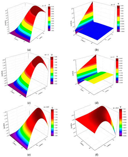
Figure 1.
Three-dimensional (3D) representation of differentiable and non-differentiable velocities defined by the multifractal model at three different fractalization degrees (σ = 0.5—(a,b); σ = 1—(c,d); σ = 5—(e,f).
2.2. Complex System Dynamics through Uniform Flow Regimes of a Multifractal Fluid
Let it be admitted that the complex system dynamics are described through uniform flow regimes of a multifractal fluid. Then, all the structural units of the complex system “support” constant velocity dynamics:
See (11) and (13) for . In this condition, (14) takes the form:
From here, for , (17) becomes:
2.3. Complex System Dynamics through Non-Uniform Flow Regimes of a Multifractal Fluid
Let it be admitted in what follows that the complex system dynamics are described through non-uniform flow regimes of a multifractal fluid (i.e., )—see Figure 1 for the 3D dependencies of the velocities, both at differentiable scale resolution (11) and at non-differentiable scale resolution (13). Now, the concurrence of the dynamics of these scale resolutions is obtained by eliminating the quadratic term in between (11) and (13), taking the form of the normalized velocity ratio:
From (19), it results that the velocity ratio homographically depends both on for ,
as well as on for :
The ratio (21) is represented in Figure 2. We observe that for lower fractalization degrees, we have a quasi-linear degree revealing the similarities between the fractal and differentiable behavior. As the fractalization degree is increased, the ratio increases and reaches saturation. The saturation moment (seen through η) is reached at η = 20 for σ = 1, while with the increase of a factor of 5 for the fractalization degree, the saturation is reached at η = 2.
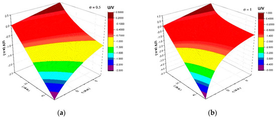
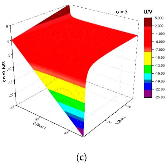
Figure 2.
Three-dimensional (3D) representation of differentiable–non-differentiable ratio defined by the multifractal model at various fractalization degrees (σ = 0.5—(a); σ = 1—(b); σ = 5—(c).
Moreover, through matrices with real elements, the functional (temporal) character becomes
and the structural (spatial) character
of the complex system.
Now, by means of (22) and (23), it is possible to operate in the complex system dynamics, with explicit differentiable descriptions, “dictated” by a metric geometry: the representations through matrices. This implies a natural metric of the matrix space; for example, for the Killing–Cartan metric of the algebra belonging to these matrices, the base covectors of such a geometry being given by means of differentiable 1-forms [32,33].
Thus, in accordance with the operational procedures [9,33], (22) implies the differentiable 1-forms:
and the multifractal structural metric:
while the (23) differentiable 1-forms:
and the multifractal functional metric:
Thus, the functional–structural coherence of the complex system dynamics, which are reducible to the multifractal space-time compatibility , implies the elimination of the multifractality degree between the metrics (25) and (27). It results, at any scale resolution, in the multifractal space-time metric:
Any of the above metrics can be generated as Caylean metrics of the Euclidean plane, taking the inner of the unit circle:
as an absolute (for details, see [34]).
Indeed, the absolute metric for the interior of the circle (29), which is:
can be assimilated to the Poincaré metric of the complex plane
based on the coordinate transformations:
Moreover, through the substitutions:
the metric (31) takes the shape:
The complex parameters and from (31) and (32) now have a direct connection with the classic theory of Newtonian-type potentials [35] based on harmonic mappings [36,37]. In order to prove this, it is needed to re-write and in the terms . It results:
The relation (35) represents harmonic mappings from the usual space to the Lobacevsky plane, having the metric (31), as long as (and thus ) are solutions of a Laplace-type equation for the free space. Indeed, the issue of harmonic mappings from the usual space to the hyperbolic plane is described through the stationary values of the Lagrangean:
specific to the variational problems:
where corresponds to the pseudo-gradient and corresponds to the infinitesimal pseudo-volume (for details see [36,37]). In such a context, the field equations result:
which admits as a solution (35). Of course, along with (38), the field equations for the complex conjugate are also satisfied.
We note also that the previous metrics written in the form:
offers the possibility of explaining the constraint for any entity of the complex system, which is engaged in a hyperbolic motion. In this case, (39) can be interpreted as absolute in the coordinates:
Indeed, for
or explicitly
the metric (31) is obtained.
The field Equation (38) with:
is equivalent with the pair of real equations:
where the differential operators are considered in a three-dimensional arbitrary metric.
As it can be observed, the constraint implies:
In this situation, the “fields” that ensure the integrity of any complex system are characterized by (45). Thus, through the change of variable , (45), in non-dimensional coordinates and for a radial symmetry, admits the solution:
Through (46) and an adequate choice of the integration constants, the solution becomes:
The relation (51) can be used to extract the coordinate in the form:
From here, at the limit , we obtain:
This result will be interpreted in the sense of the standard hyperbolic motion [37]. Then, becomes inversely proportional to the non-dimensional acceleration in the form:
As such, at , can be assimilated to an acceleration in a radial oscillatory motion or, more precisely, taking into account (51), it can be assimilated to a centripetal acceleration in a uniform circular motion.
The utilized variational principle that gives the above-mentioned result, i.e., (37), is obtained from metric (31), which is invariant when related to a certain transformation group—the group precisely (for details, see [36,37]). Now, if the functionality of the equivalence principle is admitted [37] for an arbitrary manifold point, the coordinate represents the intensity of the “fields”, while the previously mentioned group represents the transition between the various “fields” that act in that point. The appearance of the simultaneous action of these fields is a rotational motion characterized by the centripetal force (51) to the initial moment, far from the common center of the field sources.
Thus, by substituting the principle of simultaneous independent actions with the a priori invariance of the “field” action with respect to a certain group, it is possible to develop complex system dynamics theories free of any inherent contradictions found in actual theories [1,2,3].
Obviously, the analysis presented above can be extended on the metrics (25) and (27). In such a context, the structural–functional transition, at any scale resolution, is made only on geodesics of null length, , which implies the inversion . Then, (49) becomes:
Since the two types of forces that were obtained in this section (Newtonian and oscillatory type) are fundamental in the self-structuring processes of the polymer-type materials [38], in the following, we will prove that the same multifractal model will provide insight into the multiple controlled drug-release mechanisms. This will be achieved by calibrating the abstract theoretical model on empirical data.
3. Experimental Aspects
Syntheses and Investigation Methods of the Drug Delivery Systems
Diclofenac sodium salt, citral, chitosan (low molecular weight), phosphate buffer saline (pH = 7.4), and ethanol were provided by Sigma Aldrich and used without further purification. Formulations were prepared by the in situ hydrogelation of PEGylated chitosan with citral in the presence of diclofenac sodium salt, following a methodology already published [15]. Shortly afterwards, two hydrophilic PEGylated chitosan derivatives with different content of PEG reacted with hydrophobic citral in the presence of model drug, at 55 °C, under vigorous magnetic stirring. The drug amount was kept constant, while the amounts of PEGylated chitosan and citral were varied in order to assure a different ratio of the hydrophilic/hydrophobic components. The investigation of the supramolecular architecture of the systems was realized by polarized optical microscopy (POM), using a Leica DM 2500 microscope. The morphology of the samples was evaluated with a field emission scanning electron microscope (Scanning Electron Microscope SEM EDAX-Quanta 200) at accelerated electron energy of 10 eV. The in vitro release kinetic was monitored by a batch experiment performed in phosphate buffer saline (PBS) (pH = 7.4) at the human body temperature (37 °C), following a previously used experimental procedure, which mainly consisted in the determination of the percent of released drug at different moments. The experiments were done in triplicate, and the values were given as the mean value of three independent measurements. The kinetic data were fitted on several mathematic models, as follows:
- (i)
- Zero-order model: , where Qt is the amount of drug dissolved in the time t and K0 is the zero-order release constant.
- (ii)
- Higuchi model: , where Qt is the amount of drug released in the time t and KH is the Higuchi dissolution constant.
- (iii)
- Hixson–Crowell model: , where W0 is the initial amount of drug in the formulation, Wt is the remaining amount of drug in the formulation at time t, and K is a constant.
- (iv)
- Korsmeyer–Peppas model: , where Mt/M∞ is the fraction of drug released at the time t, K is the release rate constant, and n is the release exponent.
- (v)
- First-order model: , where Qt is the amount of drug released in the time t, Q0 is the initial amount of drug, and K is the first-order release constant.
4. Results and Discussions
A series of four amphiphilic formulations with different mass ratios of the hydrophilic/hydrophobic structural blocks and the same amount of model drug were prepared by condensation reaction of amines with aldehydes, and their drug release behavior was tested into an in vitro physiologic environment, according to a previously established experimental protocol [15,16].
By spectroscopic and microscopic measurements, it was established that the drug has been finely dispersed into the chitosan-based matrix due to the strong electrostatic and H-bond forces that hampered the natural tendency of crystallization of the drug. This can be easily seen in the polarizing microscopy (POM) images in Figure 3, which showed a continuous fine birefringent texture and no obvious drug crystals, which clearly indicate no phase separation of the drug in the matrix [23].
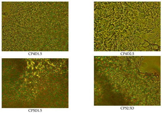
Figure 3.
POM images of the amphiphilic formulations.
The formulations displayed a porous morphology, with interconnected pores that assure favorable sink conditions of the drug (Figure 4). Moreover, the scanning electron microscopy (SEM) images confirmed the POM observations, indicating no sub-micrometric crystals into the pores or on the pore walls, suggesting a good dispersion of the drug into the matrix [18,19,20].
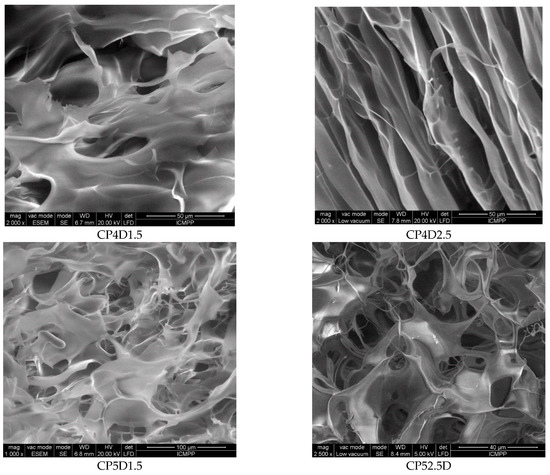
Figure 4.
SEM images of the drug release formulations.
The in vitro investigation of the drug release indicated the influence of the hydrophobic/hydrophilic balance on the release rate (Figure 5). It can be observed that the progressive increase of the hydrophilic component into formulation lead to the fastening of the drug release. Thus, the simple manipulation of the hydrophobic/hydrophilic balance can tune the drug release in agreement with the addressed requirement [15,18,19,20]. Quantitatively speaking, in 7 days, the CP4B2.5D sample released more than 99% from the entire amount of the encapsulated DCF, while the sample CP5B1.5D released only 91%—see Figure 6.
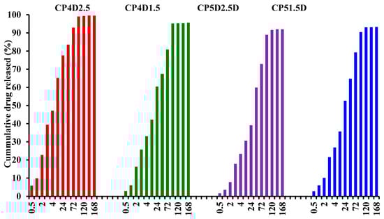
Figure 5.
The in vitro drug release in a medium mimicking the physiologic medium.

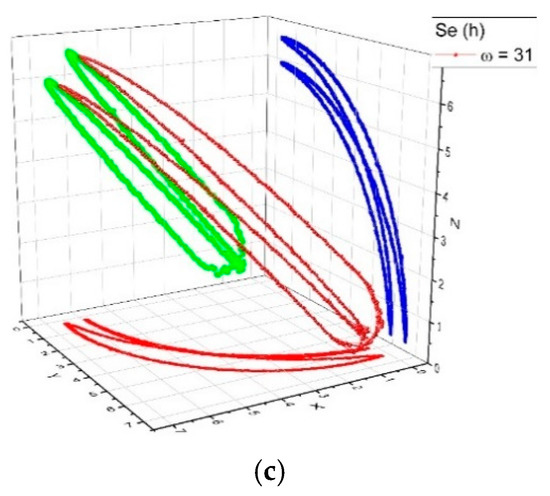
Figure 6.
Three-dimensional (3D) representation: (a) contour plot (b) and the reconstructed attractor for a period doubling type scenario (c) for drug release processes.
The fitting of the in vitro release data on the five traditional mathematical equations did not conclude on the mechanism of the drug release, as all the equations fit very well, indicating that many factors are influencing the delivery process. Concerning the theoretic model developed in Section 2, this can be validated through an adequate calibration of the empirical data, by choosing the constants according to the particularities of our polymer–drug complex system followed by a normalization of the data.
In such a context, the calibration is to be made both for the uniform and non-uniform flow regimes of the multifractal fluids. Thus, in the alternative of the uniform flow regimes of the multifractal fluid, the drug release rate of the polymer–drug complex system, , will be proportional, through (14), with the modulus of the variation velocity of the state density; for , the velocity of the multifractal fluid at a differentiable scale resolution is constant, while the velocity of the multifractal fluid at a non-differentiable scale resolution is null.
In other words, for any multifractality degree, there exists no correlation of a differentiable–non-differentiable type between the two velocity fields’ components, the release dynamics being dictated by the differentiable component of the velocity field of the multifractal fluid.
It results, through (18), the multifractal release law:
from where, for the boundary condition , it is obtained:
By retaining the first term only, then (54) becomes:
this being a result that generalizes, at any scale resolution, the “zero order” model from the standard release theories.
In the alternative of the non-uniform flow regimes of the multifractal fluid, the drug release rate of the polymer–drug complex system will be proportional, through (52), with the “intensity” of the “structural” fields for —the ratio of the velocity fields’ components for the two scale resolutions (the differentiable one and the nondifferentiable one) specifies (see (20) and (21)) the correlation through homographic transformations. Then, the polymer–drug complex system dynamics can be explained through metric geometries—the representations through matrices with real elements imply natural metrics of matrix space; by means of Killing–Cartan metrics of algebra of these matrices, the covectors bases of such geometry being given through differentiable 1-forms—see (24)–(26). Since the previously mentioned metrics can be produced as Cayleyan metrics of the Euclidean space, taking as an absolute the interior of the circle of the unity radius, between the usual and the hyperbolic space, harmonic mappings can be operated based on a variational principle—see (37) i.e., of the stationary values of the Lagrangeans—see (36) built with these metrics.
In the present context, the functionality of a variational principle is substituted to “minimal mechanisms” of release, while the solutions of the field equations corresponding to them explain not only “release scenarios”—see Figure 6 but also types of interactions responsible for release scenarios (i.e., Newtonian-type electrostatic interactions—see (24), elastic-type—see (26) etc.). In Figure 7, it is represented a release scenario build on period doubling behavior. The 3D and contour plot reveal in their temporal distribution two main structures. For each structure, a specific oscillation period is attributed. This result is better highlighted by the reconstructed attractor on which we can see clearly two oscillation periods for our evolution. Such an evolution is clearly occurring at small resolution and space-time scales that overlap the general long-time evolution of a drug-release scenario. As it can be seen in Figure 1 and Figure 2, a higher fractalization degree and small space and time coordinates with respect to the normalization parameters are perfect conditions to showcase non-differentiable behavior. The presence of a period doubling as a small-scale scenario can have an even more impactful effect on the drug delivery process. The period doubling is one of the marks for a possible transition toward a chaotic behavior. Reaching a chaotic state, it is undesirable for applications but it is worth investigating for tailoring the optimum release conditions.
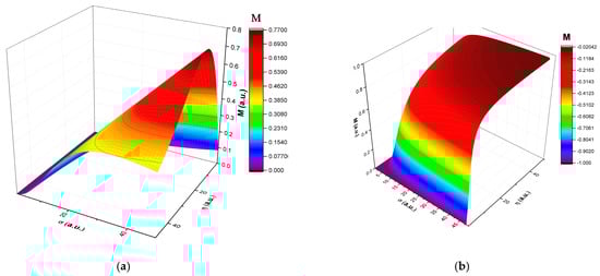
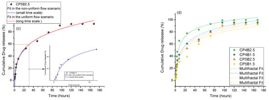
Figure 7.
Simulated drug delivery dynamics in the uniform flow scenario and simulated drug delivery dynamics in the non-uniform flow scenario.
From such a perspective, through (52) results the multifractal release law:
In Figure 7, we have represented the simulated drug mass release (53) in Figure 7a and (56) in Figure 7b, and the multifractal fit of the drug release empirical data at different temporal scales (Figure 7c) and for various polymer-drug configurations (Figure 7d) We notice when representing the two equations as functions of normalized time and space an increase and saturation for the global function, while the localized function is described by a maximum drug release induced by the fractalization degree of the system. These two models need to be understood sequentially, as experimentally, it is seen that releases on relatively short times can be different than the overall recorded values.
In what follows, let the empirical data be calibrated to the theoretical model based on relations (53) and (56) (Figure 7). Since we notice that (see Figure 3 and Figure 4) the polymer–drug complex system can be structurally associated to a multifractal object, we can consider that the polymer–drug complex system behaves, from a functional point of view, as a multifractal. The calibration process is not a trivial one, as it strictly depends on the nature of the investigated phenomena. This method was previously tested for other physical phenomena with promising results [39] and cemented the fractal approach as a truly versatile one that can intimately describe the dynamic behavior of complex systems. It can be observed that the model fits well the CPD2.5, where the saturation region is reached earlier. This is also due to the morphology of the formulation, which has a more organized structure, enhancing the release. This, translated into the fractal paradigm used for the theoretical model, means that a non-fractal morphology will lead to a higher fractality in the geodesics of the release drugs as it enhances the interactions between the drug and the release media. As the morphology of the polymer formulations becomes fractalized (see Figure 5), the release is reduced, and the overall fractalization degree of the drug-release is reduced—see Figure 7. Let it be noted that the calibration of the author’s model works well also on short evolution times (<20 h) with the mention that the fractalization degree does not depend on the time scale, as the fractality is not a measure of the time scale but rather describes the polymer–drug system.
5. Conclusions
Using the Multifractal Theory of Motion developed by means of the multifractal hydrodynamic equation, complex system dynamics were analyzed through uniform and non-uniform flow regimes. For the description of the uniform flow regime of the multifractal fluid, the dynamics are “supported” only by the differentiable component of the velocity field, while the non-differentiable was considered null. In the case of the non-uniform flow regime of the multifractal fluid, the dynamics is “supported” by both components of the velocity field, their ratio specifying correlations through homographic transformations. The transformations imply metric geometries explained by means of Killing-Cartan metrics of the -type algebra, of the set of matrices with real elements. Since these metrics were “produced” as Cayleyan metrics of absolute geometries, the dynamics description is reducible, based on a minimal principle, to harmonic mappings from the usual space to the hyperbolic space. The theoretical model is calibrated based on empirical data of an amphiphilic matrix based on chitosan, which was developed to control drug release applications. An amphiphilic matrix based on chitosan was developed, and its ability for controlled drug release applications was investigated. The investigated systems demonstrated a lack of any in vivo toxicity encouraging further investigations of the laws that govern their ability to function as an efficient matrix. However, future studies are needed in order to establish its applications in endometriosis or intrauterine adhesions management.
Author Contributions
Conceptualization, M.A. and D.V.; methodology, D.F., C.E.G.-I. and A.I.V.; software, D.V. and T.-C.P.; formal analysis, A.Z. and L.D.; investigation, C.B.; resources, A.Z. and L.D.; writing—original draft preparation, T.-C.P.; writing—review and editing, M.A. and T.-C.P.; supervision, M.A. and T.-C.P.; All authors have read and agreed to the published version of the manuscript. Furthermore, all the authors have the same weighted contribution to the manuscript.
Funding
This research received no external funding.
Institutional Review Board Statement
Not applicable.
Data Availability Statement
The data will be available from the corresponding author on request.
Acknowledgments
We would like the acknowledge the referees’ insightful observation and comments, which helped improve the paper.
Conflicts of Interest
The authors declare no conflict of interest.
References
- Bar-Yam, Y. Dynamics of Complex Systems; Apple Academic Press: Cambridge, MA, USA, 2019. [Google Scholar]
- Mitchell, M. Complexity: A Guided Tour; Oxford University Press: Oxford, UK, 2009. [Google Scholar]
- Badii, R. Complexity: Hierarchical Structures and Scaling in Physics; Cambridge University Press: Cambridge, UK, 1997. [Google Scholar]
- Flake, G.W. The Computational Beauty of Nature; MIT Press: Cambridge, MA, USA, 1998. [Google Scholar]
- Băceanu, D.; Diethelm, K.; Scalas, E.; Trujillo, H. Fractional Calculus, Models and Numerical Methods; World Scientific: Singapore, 2016. [Google Scholar]
- Ortigueria, M.D. Fractional Calculus for Scientists and Engineers; Springer: Berlin/Heidelberg, Germany, 2011. [Google Scholar]
- Nottale, L. Scale Relativity and Fractal Space-Time: A New Approach to Unifying Relativity and Quantum Mechanics; Imperial College Press: London, UK, 2011. [Google Scholar]
- Merches, I.; Agop, M. Differentiability and Fractality in Dynamics of Physical Systems; World Scientific: Hackensack, NJ, USA, 2016. [Google Scholar]
- Agop, M.; Merches, I. Operational Procedures Describing Physical Systems; CRC Press: Boca Raton, FL, USA, 2019. [Google Scholar]
- Politi, A.; Pikovsky, A. Lyapunov Exponents: A Tool to Explore Complex Dynamics; Cambridge University Press: Cambridge, UK, 2016. [Google Scholar]
- Cruzeiro, A.B. Stochastic Approaches to Deterministic Fluid Dynamics: A Selective Review. Water 2020, 12, 864. [Google Scholar] [CrossRef]
- Gaite, J. The Fractal Geometry of the Cosmic Web and Its Formation. Adv. Astron. 2019, 2019, 6587138. [Google Scholar] [CrossRef]
- Shahzad, M.U.; Iqbal, A.; Jawad, A. Dynamical Properties of Dark Energy Models in Fractal Universe. Symmetry 2019, 11, 1174. [Google Scholar] [CrossRef]
- Mandelbrot, B.B. The Fractal Geometry of Nature; W.H. Freeman and Co.: San Francisco, CA, USA, 1982. [Google Scholar]
- Iftime, M.M.; Dobreci, D.L.; Irimiciuc, S.A.; Agop, M.; Petrescu, T.; Doroftei, B. A theoretical mathematical model for assessing diclofenac release from chitosan-based formulations. Drug Deliv. 2020, 27, 1125–1133. [Google Scholar] [CrossRef] [PubMed]
- Marin, L.; Ailincai, D.; Mares, M.; Paslaru, E.; Cristea, M.; Nica, V.; Simionescu, B.C. Imino-chitosan biopolymeric films. Obtaining, self-assembling, surface and antimicrobial properties. Carbohydr. Polym. 2015, 117, 762–770. [Google Scholar] [CrossRef] [PubMed]
- Chen, A.; Samankumara, L.P.; Garcia, C.; Bashaw, K.; Wang, G. Synthesis and characterization of 3-O-esters of N-acetyl-d-glucosamine derivatives as organogelators. New J. Chem. 2019, 43, 7950–7961. [Google Scholar] [CrossRef]
- Ailincai, D.; Mititelu, L.T.; Marin, L. Drug delivery systems based on biocompatible imino-chitosan hydrogels for local anticancer therapy. Drug Deliv. 2018, 25, 1080–1090. [Google Scholar] [CrossRef] [PubMed]
- Ailincai, D.; Mititelu-Tartau, L.; Marin, L. Citryl-imine-PEG-ylated chitosan hydrogels—Promising materials for drug delivery applications. Int. J. Biol. Macromol. 2020, 162, 1323–1337. [Google Scholar] [CrossRef] [PubMed]
- Iftime, M.-M.; Tartau, L.M.; Marin, L. New formulations based on salicyl-imine-chitosan hydrogels for prolonged drug release. Int. J. Biol. Macromol. 2020, 160, 398–408. [Google Scholar] [CrossRef] [PubMed]
- Wu, Y.; Rashidpour, A.; Almajano, M.P.; Metón, I. Chitosan-Based Drug Delivery System: Applications in Fish Biotechnology. Polymers 2020, 12, 1177. [Google Scholar] [CrossRef] [PubMed]
- Guyot, C.; Cerruti, M.; Lerouge, S. Injectable, strong and bioadhesive catechol-chitosan hydrogels physically crosslinked using sodium bicarbonate. Mater. Sci. Eng. C 2021, 118, 111529. [Google Scholar] [CrossRef] [PubMed]
- Dimitriu, D.G.; Irimiciuc, S.A.; Popescu, S.; Agop, M.; Ionita, C.; Schrittwieser, R.W.; Stefan-Andrei, I. On the interaction between two fireballs in low-temperature plasma. Phys. Plasmas 2015, 22, 113511. [Google Scholar] [CrossRef]
- Irimiciuc, S.A.; Agop, M.; Nica, P.; Gurlui, S.; Mihaileanu, D.; Toma, S.; Focsa, C. Dispersive effects in laser ablation plasmas Japan. J. Appl. Phys. 2014, 53, 116202. [Google Scholar] [CrossRef]
- Feynman, R.P.; Hibbs, A.R.; Weiss, G.H. Quantum Mechanics and Path Integrals. Phys. Today 1966, 19, 89. [Google Scholar] [CrossRef]
- Bohm, D. Quantum Theory; Constable: London, UK, 1954. [Google Scholar]
- van den Berg, J.C. Wavelets in Physics; Cambridge University Press: Cambridge, UK, 2004. [Google Scholar]
- Hilborn, R.C. Chaos and Nonlinear Dynamics; Oxford University Press: Oxford, UK, 1994. [Google Scholar]
- Agop, M.; Nica, P.E.; Gurlui, S.; Focsa, C.; Paun, V.P.; Colotin, M. Implications of an extended fractal hydrodynamic model. Eur. Phys. J. D 2009, 56, 405–419. [Google Scholar] [CrossRef]
- Irimiciuc, S.; Bulai, G.; Agop, M.; Gurlui, S. Influence of laser-produced plasma parameters on the deposition process: In situ space- and time-resolved optical emission spectroscopy and fractal modeling approach. Appl. Phys. A 2018, 124, 615. [Google Scholar] [CrossRef]
- Cobzeanu, B.M.; Irimiciuc, S.; Vaideanu, D.; Grigorovici, A.; Popa, O. Possible Dynamics of Polymer Chains by Means of a Ricatti s Procedure—An Exploitation for Drug Release at Large Time Intervals. Mater. Plast. 2017, 54, 531–534. [Google Scholar] [CrossRef]
- Hilgert, J.; Neeb, K.-H. Structure and Geometry of Lie Groups; Springer Science: New York, NY, USA, 2012. [Google Scholar]
- Gallier, J.; Quaintance, J. Differential Geometry and Lie Group; Springer International Publishing: New York, NY, USA, 2020; Volume 12. [Google Scholar]
- Onishchik, A.L.; Sulanke, R. Projective and Cayley-Klein Geometries; Springer: Berlin/Heidelberg, Germany, 2006. [Google Scholar]
- Agop, M.; Gavriluț, A.; Grigoraș-Ichim, C.; Toma, Ș.; Petrescu, T.-C.; Irimiciuc, Ș.A. Toward Interactions through Information in a Multifractal Paradigm. Entropy 2020, 22, 987. [Google Scholar] [CrossRef] [PubMed]
- Xi, Y. Geometry of Harmonic Maps; Springer: New York, NY, USA, 2018. [Google Scholar]
- Misner, C.W.; Thorne, K.S.; Wheeler, J.A. Gravitation; W.H. Freeman: San Francisco, CA, USA, 2018. [Google Scholar]
- Israelachvili, J.N. Intermolecular and Surface Forces; Academic Press: New York, NY, USA, 2011. [Google Scholar]
- Irimiciuc, S.A.; Nica, P.-E.; Agop, M.; Focsa, C. Target properties—Plasma dynamics relationship in laser ablation of metals: Common trends for fs, ps and ns irradiation regimes. Appl. Surf. Sci. 2020, 506, 144926. [Google Scholar] [CrossRef]


Publisher’s Note: MDPI stays neutral with regard to jurisdictional claims in published maps and institutional affiliations. |
© 2021 by the authors. Licensee MDPI, Basel, Switzerland. This article is an open access article distributed under the terms and conditions of the Creative Commons Attribution (CC BY) license (https://creativecommons.org/licenses/by/4.0/).