Abstract
Traffic microsimulation models use the movement of individual driver-vehicle-units (DVUs) and their interactions, which allows a detailed estimation of the traffic noise using Common Noise Assessment Methods (CNOSSOS). The Dynamic Traffic Noise Assessment (DTNA) methodology is applied to real traffic situations, then compared to on-field noise levels from measurement campaigns. This makes it possible to determine the influence of certain local traffic factors on the evaluation of noise. The pattern of distribution of vehicles along the avenue is related to the logic of traffic light control. The analysis of the inter-cycles noise variability during the simulation and measurement time shows no influence from local factors on the prediction of the dynamic traffic noise assessment tool based on CNOSSOS. A multifractal approach of acoustic waves propagation and the source behaviors in the traffic area are implemented. The novelty of the approach also comes from the multifractal model’s freedom which allows the simulation, through the fractality degree, of various behaviors of the acoustic waves. The mathematical backbone of the model is developed on Cayley–Klein-type absolute geometries, implying harmonic mappings between the usual space and the Lobacevsky plane in a Poincaré metric. The isomorphism of two groups of SL(2R) type showcases joint invariant functions that allow associations of pulsations–velocities manifolds type.
1. Introduction
It is well known that the main source of noise in urban areas is due to road traffic [1,2]. Figures on the number of vehicles in European cities continue to increase, leading to major pollution problems. The incorporation of electric vehicles is not happening at the same rate in all countries. When it comes to noise pollution, according to the 2018 studies (EU-28), it seems that approximately 75 million people within urban areas are exposed to a noise level Lden (day–evening–night) above 55 dB [1].
The consequences of noise exposure of city inhabitants are often ignored or underestimated. The impact of traffic noise on humans is related to its negative impact on their health and behavior. There is growing evidence proving that noise is a cause of annoyance, nervousness, stress, sleep disturbance, decreased professional performance, and reduced learning ability of children [3,4,5,6,7,8]. Not all noise-related health problems mean hearing loss, serious health problems have also been reported due to prolonged noise exposures that cause, among others, high blood pressure, cardiovascular accidents, diabetes, even mental health problems [9,10,11,12]. Regarding the European Environment Agency using data of the year 2017, the situation in Romania concerning the number of inhabitants with sleep problems and annoyed by noise is very important. In this regard, the figures for assessing the impact of traffic noise on human health in Romanian conurbation are very worrying [2].
The European Noise Directive [13] is based on three pillars that address the diagnosis, information to the public, and the treatment of problems that arise from environmental noise. To complete the task, a methodological plan is developed that adopts a “macro” approach when spatially analyzing the distribution of noise in the city and adopts a “long-term” perspective when the dose of noise exposure is evaluated. In a medium-sized city (Bacau, Romania), two rounds of strategic noise maps have been carried out, the first is from 2012 and the second from 2018 [14]. The results of the estimation of the number of inhabitants exposed to traffic noise are the ones expressed in Table 1 for the day–evening–night noise levels Lden and night noise levels Lnight.

Table 1.
Summary of results Lden and Lnight of exposure to noise to traffic noise within the Bacau urban area [14].
By applying the amendment 2020/367 [15] of the Directive 2002/49/EC, the figures of people affected by the harmful effect due to road noise are as follows:
Table 2 presents the occurrence of harmful effects in a population exposed in Bacau to levels Lden > 55 dB and Lnight > 50 dB. For the calculations, HA (high annoyance) and HSD (high sleep disturbance) were used, using dose–effect relations set out in this amending to Noise Directive. Finally, the total number of people (N) affected by these harmful effects (HA and HSD) due to road noise (Lden and Lnight) was estimated. These indicators are based on previous works that have been endorsed by the WHO [16,17]. Comparison of figures presented in Table 1 and Table 2, suggests either a growth in noise, or a growth in population, or both. The increase of 33,140 people exposed to Lden > 55 dB and 44,588 people exposed to Lnight > 50 dB over these 6 years, warns that something needs to be done to reduce noise.
Table 2.
Summary of results of the total number of people affected by the harmful effect due to traffic noise within the Bacau urban area.
Another concern found in the literature that evaluates the nuisance by traffic noise in the population is that the long-term traffic noise indicators (Lden, Lnight) cannot explain by themselves all the adverse effects that traffic noise causes in the population. For this reason, there is a growing need to explore other characteristics of traffic noise that are also causes of annoyance, sleep disturbances, and health problems, for example, low-frequency noise [18,19,20]. Low-frequency content is relatively more dominant indoors and behind noise barriers where mid-high frequency content is reduced. Paradoxically, even if the overall noise level goes down, the annoyance and complaints from people may increase. Moreover, the high spatial–temporal variability of traffic noise makes it advisable to take into account the possibility of using also other noise indicators that can better assess certain aspects of annoyance not clearly included in the static strategic noise maps [21]. Road traffic noise depends on several well-known factors, such as traffic density, vehicle fleet composition, speed, and speed variations. The road surface and the type of tires should also be considered. When the flow of vehicles involves frequent speed changes, including stop and go conditions, it usually involves the generation of noise events [22,23,24]. This adverse phenomenon can be quantified in terms of the levels and number of these noise events using the maximum noise levels LAFmax exceeding a threshold or time history of LAeq,T=1s.
There are many examples of studies within the literature that make evaluations of specific noise problems using alternative noise indicators together with dynamic tools capable of micro-analysis of noise issues [25,26,27,28,29,30,31,32,33,34]. Therefore, the main objective of the current study is to analyze the validity and applicability of CNOSSOS-EU road noise emission model [35] for noise road traffic prediction in the urban area of a medium-sized city (Bacau, Romania). In first place, it will be verified whether the methodology called Dynamic Traffic Noise Assessment tool or, for short, DTNA tool is capable of correctly modeling the noise emitted by mixed traffic in an area regulated by traffic lights, with constant accelerations and decelerations on a city avenue of Bacau. On the other hand, a multifractal model of acoustic waves propagation is proposed that assumes the role of simulating the external constraints that can be found in real acoustic waves.
Another objective of this study aims to demonstrate the limitations of conventional strategic noise maps to show the data necessary to (i) assess the level of annoyance, (ii) understand the scope of the problem, and then, (iii) propose the appropriate measures noise mitigation.
2. Traffic Noise Standard Model
Any new methods used for the analysis of noise mitigation measures must be tested. Their effectiveness should be subjected to validation when it is suspected that local factors may have an impact on a correct evaluation. In this part of the study, it is intended to check if the noise dynamic emission model of CNOSSOS will have problems predicting the real emissions of road traffic in the city of Bacau. This question on which the research is founded is based on two facts: (i) the vehicles in this region are very old, and (ii) the aggressive driving behavior of car drivers. For this reason, a section of an avenue was selected in the city where there are frequent speed changes, with accelerations and decelerations. Therefore, it is necessary to carry out field studies that measure the performance parameters. For this, a series of trials were defined controlling all the variables involved. The possibilities and also the limits of the use of the DTNA tool in the city of Bacau (and, by extension, in many cities in Romania) must undergo a validation process. This tool is proposed in previous works [25,26,27,28,29,30,31,32,33,34]. Once the limits of the method have been tested, it will be used to generate dynamic noise maps in CADNA that more realistically analyze the proposed mitigation measures for traffic noise.
The validation implies:
- -
- Carrying out a noise measurement campaign in a section of an avenue in the city of Bacau that stands out for its importance in the strategic noise map of this agglomeration.
- -
- Generation of a VISSIM traffic model for the avenue, with the traffic conditions identified at the moment when the noise measurements are performed;
- -
- Calculation of noise power of traffic flow using DTNA tool (performed in VISSIM-MATLAB combination);
- -
- Recreation of a virtual sound level meter that mimics the actual position of the microphone during the noise/traffic measurement campaign and estimation of noise levels at that point;
- -
- Noise mapping of the avenue using NMPB (French road traffic noise prediction model) and CNOSSOS (Common Noise Assessment methods developed under the European Commission umbrella);
- -
- Statistical and comparative analysis of the two evaluation methods (measurements and simulation);
- -
- Comparative analysis of the different approaches respects the official strategic noise maps.
2.1. Study Area: Marasesti Avenue in Bacau
The document prepared to design the action plans in the city points out some traffic noise hot-spots that are identified in the city through the strategic noise maps [14]. For this, it warns that the total number of people exposed to levels that exceed the limit values of 70 dBA for the Lden indicator, is 29,251. At the same time, the number of people living exposed to more than 60 dBA for the Lnight is 36,189. These people live along several arteries of the city including the Calea Marasesti.
For the choice of this avenue, this evidence was taken into account. Figure 1 shows a 3-D representation of the study area imported from CADNA (Computer Aided Noise Abatement software). It shows the selected study area in Marasesti Avenue. The noise measurement position is defined in the image with a white arrow.
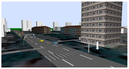
Figure 1.
3-D representation of the study area imported from CADNA (Computer Aided Noise Abatement software).
Besides, the analyzed section of the avenue has some characteristics that made it suitable for the study.
- -
- The surface of the avenue is in good condition and is neutral for the generation of noise.
- -
- The traffic flow includes a small percentage of heavy vehicles, mainly composed of buses.
- -
- The avenue is straight and from the perspective of the measuring point, there are no obstacles (upstream/downstream) between the vehicles passing through the avenue and the microphone.
- -
- The surrounding land surface is flat.
- -
- There are no significant vertical reflective surfaces in the vicinity of the sound level meter.
- -
- Regarding noise zoning and city area, it should be noted that the location is in the downtown of the city, and the land use around the avenue is mainly residential. Although, there is an area that must be considered sensitive.
- -
- Lane width is 3.5 m. Speed limit—50 km/h.
- -
- A traffic light is in the area that makes traffic flow not regular with speed changes.
2.2. Noise Measurement Design
The sound level meter used in the determination of the traffic noise level (including cables, microphone, and preamplifier) meets the requirements of a type 1 instrument, as defined by European standards EN-60651: 1996 modified by EN-60804 /A1: 1997 and EN-60804: 1996 modified by EN-60804/A2: 1997. It is the Bruel and Kjaer 2270 with the microphone B&K 4189 and the Extended Sound Analysis Software B&K BZ-7225. The B&K 2270 was used together with a tripod and wind protection. Before and at the end of each measurement the status of the measurement chain was verified using the calibrator B&K 4231. For the collection of local weather conditions during noise measurements, the meter Testo 425 was used. The variables collected were the wind speed, the relative humidity, and the temperature. The general wind direction and atmospheric pressure were collected from nearby meteorological stations.
Noise tests were carried out to validate the emission model, so the measurement point where the effect of noise propagation is minimized as much as possible was selected. In general, the test design follows the precepts and recommendations of the international standard ISO 1996-2:2017 Acoustics—Description, measurement, and assessment of environmental noise—Part 2: Determination of sound pressure levels.
Spatial sampling considerations:
- -
- The position of the microphone was specified following the HARMONOISE methodology [36], 7.5 m from the centerline of the closest lane.
- -
- The measuring point was chosen in front of the stop line of vehicles (the traffic light stop line S–N direction).
- -
- The measurement point was selected away from building facades and vertical walls, and therefore it will not be necessary to correct for reflection.
- -
- The viewing angle of the microphone on the road is greater than 150 degrees.
- -
- The measuring height where the microphone is situated is 1.3 m.
Time sampling considerations:
- -
- Noise magnitude (equivalent continuous sound level) is recorded LAeq, T = 1 s. Noise spectra in third-octave bands are also registered but not considered for the study purpose.
- -
- Three measurement campaigns of 1 h and 30 min were carried out on different days. From these campaigns, a record of 1 h duration was extracted (actually a noise time series of 3630 noise data), once all noise anomalies not due to traffic were discarded and it was guaranteed that the vehicle set follows the statistics of the region. When an anomaly is detected, the entire traffic light cycle included is deleted.
Noise source considerations:
- -
- The traffic flow is made up of heavy and light vehicles.
- -
- The capacity of Marasesti Avenue allowed by the traffic signaling cycle and the traffic density at the time of measurement guarantee a fluid traffic flow, far away from congestion.
- -
- The choice of the season of the year in which the noise measurement campaigns are carried out ensures that the tires of the vehicles during the test are not for winter use.
2.3. Complementary Equipment Used to Describe Traffic
The main measuring equipment was used to characterize the traffic noise and, in a synchronized way, the complementary equipment identifies the traffic variables related to that noise (Figure 2). Complementary measuring equipment is understood as the one that has the purpose of guaranteeing the repetitiveness and reproducibility of the environmental noise tests coming from the traffic. The equipment used in the test are as follows:
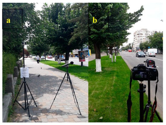
Figure 2.
Camera for video-audio recording and the sound level meter B&K 2270 (a). Radar gun Stalker ATS II and Canon camera (b).
- -
- For vehicle speed and acceleration measurements—Radar gun Stalker ATS II + Canon camera.
- -
- For vehicle description and classification of driver’s behavior through video and audio recording—GoPro HERO 2 with a tripod which is a 170° wide-angle lens.
All the equipment shown in Figure 2 was programmed to provide data in a synchronized way. With the video and audio from the camera, the traffic situation can be recreated as many times as desired. The traceability of traffic variables environmental noise test by audio and video is synchronized with the acoustic measurements. This way the number of vehicles and their category during the test can be established. The audio helps to identify the source of the noise recorded by the sound level meter, synchronize the events, and interpret the scene of the video and in the conditions in which the events occurred. With this combination audio–video–noise record, the idle noise episodes can be identified when the cars are at the traffic light. We discarded noise episodes that do not correspond to traffic noise. At the same time, the age of the cars that have been part of the study, whether they are gasoline or diesel, the type of vehicle, etc., can be checked. With this, it can be guaranteed that the test situation corresponds to the statistics handled for the vehicle park. The behavior of the drivers can be also analyzed and the other calibration data can be recovered if necessary, as the length of queues, the reaction time of the driver, changes in traffic light programming, etc.
The identification and marking of residual noise are facilitated by audio/video recordings. Once these events are marked, they can be discarded. During the measurements, anomalies took place as vehicles that commit infractions (prohibited U-turns), shouts of people, ambulance–police sirens, and horns.
2.4. Dynamic Traffic Noise Assessment (DTNA) Tool
VISSIM simulation is the heart of the methodology of the dynamic noise prediction tool. Traffic micromodels simulate the movements (axial and lateral) of every driver-vehicle unit (DVU) in the street and their interaction with the rest of DVUs. In micro-simulation traffic models, every vehicle is modeled individually and its position, acceleration, and speed are updated in discrete time steps. That is why noise associated with a certain street is a function of space/time evolution of sound power levels emitted by every vehicle in the street (see Figure 3). In the present study, 1-h output data from VISSIM (vehicle type, position, time, speed, and acceleration) was introduced in a MATLAB script and using the two HARMONOISE-IMAGINE-CNOSSOS [35,37,38] Equation (1) for rolling noise power and (2) for engine noise power, and taking into account the latest recommendations and precautions for the implementation of the method [39,40], the noise power of the selected road section is identified.
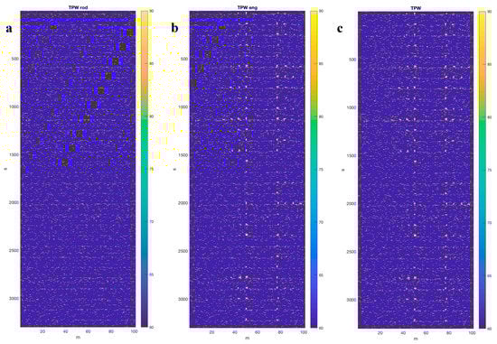
Figure 3.
Space/time evolution of LAw (t, s).
LWR is the rolling (tire/road) noise power; AR and BR are the coefficients that will change for each frequency band “f” in octaves for each vehicle category; v is the speed of the vehicle, and vref is the reference speed.
LWP is the propulsion noise power, AP, BP, CP are coefficients that will change for each frequency band “f” in octaves for each vehicle category; v is the speed of the vehicles; vref is the reference speed; a represents the acceleration of the vehicle.
The results from CNOSSOS road noise emission model (noise power) serve, at first, as input to a simplified propagation model that allows determining the sound pressure levels at a receiver point that mimics the exact position of the sound level meter with respect to the track. This will estimate the measured sound pressure levels, LAeq (every 1 s) by the virtual sound level meter, second by second in the analysis time interval (1 h). Figure 3 helps to understand how the noise power distribution, LAw, along the avenue, evolves (in this case it was only shown 101 m centered on the measurement point), second by second, during the simulation time. It is interesting to note that the traffic light situation and the duration of the traffic light cycle can be deduced from the graph itself, paying attention to the patterns (periodicities) revealed in the space–time distribution of noise power emissions.
The graphs (Figure 3) present, from left to right, the temporal evolution of LAw (t, s), the radiated power per meter, and, per second, at 101 m around the measurement point (s = 51 m where is the traffic light). The noise power at the source is due to the traffic composition except for motorcycles and other special vehicles. In the case on the left (a), it is shown the rolling noise, on the center the engine noise, and on the right (c) the total power. The “x” axis is the space (s) that coincides from left to right with the S–N direction. The “y” axis represents the progression in time (t) from the top (1 s) to the bottom (until 3630 s). The colors represent the sound power level from highest (tending towards yellow) to lowest (tending towards dark blue)
2.5. Local Factors
VISSIM is the traffic microscopic model used in this paper. Nonetheless, to obtain a more realistic approach to noise emissions, micro-simulation traffic models strongly depend on some constraints [41]:
- A technical description of every vehicle class that participates in traffic flow during the time of noise measurements.
- Credible modeling of actions and interactions between vehicles.
- A detailed description of the network, its traffic control features (i.e., signal timing, signs), and rules.
- A correct geographic layout (UTMx and UTMy coordinates) for the construction of the network.
- Traffic volume and composition of the fleet in every link and node of the network.
- Calibration data (traffic counts distinguishing all modes, speed, the length of queues, etc.).
Through the work done with the equipment used on-site, and after the necessary processing, the traffic constraints 2–6, could be measured in the case study. The aggressiveness of the drivers can be credited by measuring accelerations, decelerations, and cruise speed. The following was also defined: reaction times, the minimum distance to the vehicle in front, and lane changes of each driver. Unfortunately, not all the software packages provide adjustable interfaces for the parameters that define the behavioral model [42] or, at least, an interface to use optional external driver models.
About constraint 1, the DTNA tool should include a technical breakdown of every vehicle class and its noise emission. According to a recent study, the North-East Region of Romania has the lowest level of motoring (177 passenger cars per 1000 inhabitants) compared to other regions. Despite this fact, the motorization index of Bacău city (368 cars per 1000 inhabitants) is well above this motoring index and increasing, the average of the motorcycle rate in the last 5 years is 3.3% (https://www.drpciv.ro). Although there is a continuing increase in car fleet, the percentage of cars with 5 years as the maximum age is only 5% (https://www.drpciv.ro). Nowadays, Bacau vehicle park carries approximately 74,000 vehicles, according to the Vehicle Driving and Registration Regime (https://municipiulbacau.ro/wp-content/uploads/2017/09/04.proiect-mud-partea-3.pdf).
Therefore, Bacau has a fleet of old cars, with many second-hand vehicles that, together with aggressive driving behavior, give rise to the following questions to be considered in this work. Will CNOSSOS road noise emission model, Equations (1) and (2), work correctly for the calculation of the noise power emitted by traffic in the streets and avenues of the city of Bacau without the need to introduce any correction? Taking into consideration that at low speed, the propulsion noise is the predominant one, if there is any difference in the emitted noise by the vehicle fleet due to other local factors, it will be noticeable more in stop and go situations when vehicles have enough room for strong accelerations. Some research groups have conducted studies that assess the variability of the emissions due to the distinctive characteristics of the fleet [43,44,45]. This dispersion of results is more important when the LAFmax record is evaluated for noise action plan purposes.
3. Model Results
3.1. Results of the Measurement Campaign Traffic Variables
The real traffic conditions are very important to correct the VISSIM model until reaches a degree of realism in Bacau. The incorporation of this data reproduces a more realistic behavior model of the vehicle–driver unit for the time when the environmental noise test was carried out. The real traffic density was identified during the measurements and is shown in Table 3.
Table 3.
Traffic data identified during the measurements and considered in the simulation.
The distribution of the car speed (Figure 4) shows the many light vehicles driving with a speed greater than 50 km/h which is the regulation on the respective section of the avenue. This is not the case for heavy vehicle speed (Figure 5). It can be concluded that there is a high percentage of aggressive driving (Table 4).
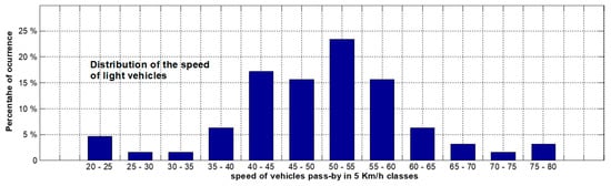
Figure 4.
Cars speed distribution during test time (cruising speed).
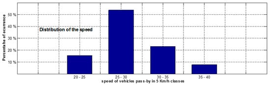
Figure 5.
Heavy vehicle speed distribution during test time (cruising speed).
Table 4.
Driving behavior distribution.
Other important data recovered is the following:
- -
- The traffic signal program remains the same during all noise measurement campaigns. The total cycle time of 110 s is distributed as follows: 86 s of green time, 4 s of yellow, and 20 s of red.
- -
- The queues of vehicles stopped in front of the traffic light have never exceeded seven vehicles.
- -
- No Medium-Heavy vehicles were detected.
- -
- Motorcycles and special vehicles not of interest in the analysis were not taken into account.
3.2. Results of the Noise Measurements Campaign
From the measurements carried out in the field, 1 h of noise data was obtained. The LAeq,T=1s data record is the one shown below in Figure 6 and Figure 7.
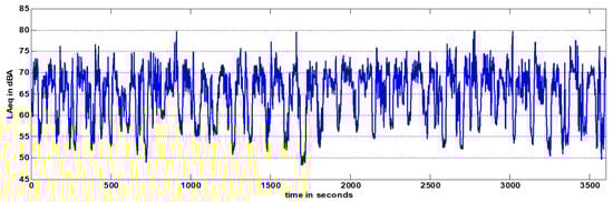
Figure 6.
Noise measurements in the exterior once the anomalies produced by ambulances, sirens, motorcycles, and other events that cannot be simulated in VISSIM have been corrected.
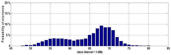
Figure 7.
LAeq,T=1s distribution per noise level classes, once the noise anomalies have been corrected.
3.3. Noise Results Coming from Traffic Noise Simulation in the Selected Area
VISSIM must simulate the traffic that has been collected on the street in relation to the configuration of the road, traffic lights, and the number of vehicles, and the composition of the fleet. Something very important is to incorporate the actual parameters of cruising speed and acceleration. Concerning the control of the traffic light, special attention is paid to realistically include the traffic lights upstream and downstream of the study area (and that are not seen in the images) that are the cause of the composition of the platoons and have a special impact on the temporal evolution of noise in the area.
This does not only refer to the instantaneous speed but the cruising speed that the drivers intend to reach on an avenue with traffic lights. For its estimation, only the speed of the vehicles leading the traffic platoons was chosen, as the rest is subject to maintaining this speed and therefore does not add information in this regard.
The time series (shown in Figure 8) was generated after applying the simulation method and finally using a MATLAB script that generates the data of acoustic levels registered in a virtual sound level meter that mimics the real situation, as they were recorded. Distribution of the values shown in Figure 8 and Figure 9 are as follows: LAeq,T=3630s = 68.6 dBA, arithmetic mean 65.77 dBA, standard deviation = 5.32 dBA.
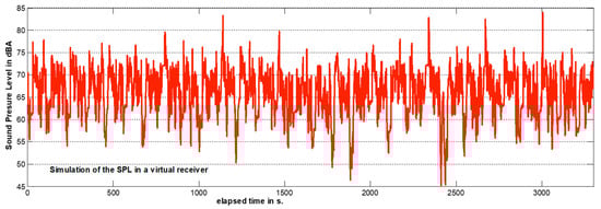
Figure 8.
The 3630 values of LAeq,T=1s recorded by the virtual sound level meter located in the same position as the real one shown in Figure 2.
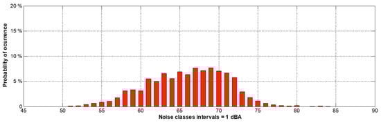
Figure 9.
Distribution of LAeq,T=1s data shown in Figure 8 (per noise level classes).
3.4. Noise Maps
For comparison reasons, the maps were prepared with the same methodology as the official strategic noise maps of Bacau. They were estimated for a case study area and using the traffic data collected in the measurement campaign (Figure 10). Marasesti Avenue in Bacau was introduced for a section of 401 m. First, the noise traffic map was generated with the NMPB96 model, as it was employed in the two rounds of Bacau strategic noise maps. Then, to show the difference with the CNOSSOS model, the traffic noise map using the same input data (geometrical and attribute data) was also presented using CADNA sound prediction software.
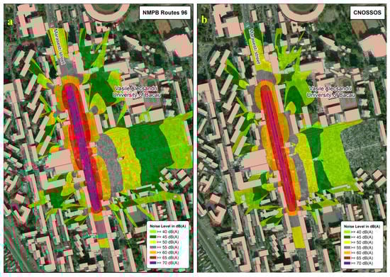
Figure 10.
LAeq,T=1h noise map built with collected traffic information recovered during the measurements campaign. On the left (a), the map prepared with the provisional traffic noise model NMPB06. On the right (b), the map prepared with the current traffic noise model CNOSSOS.
The noise maps developed by DTNA were also estimated. The improvement is to describe the sound levels variations instead of a static description of road traffic noise as it is usual in strategic noise mapping in Figure 10, where LAW (noise power per meter) remains constant along the avenue. Examining the average sound power along the 401 m of the simulated path during the 3630 s of analysis, it can be extracted that the noise fluctuations describe a periodicity that corresponds to the traffic light period.
If noise power emission is averaged per 33 cycles during the 110 s of traffic light cycle, this process can generate 110 intra-cycle noise maps for every second of the cycle. Figure 11 represents two of these possible maps, those built with the minimum and maximum total noise power associated with the street. The maps were created using the CNOSSOS propagation model and give a time-dependent vision of the dispersion of noise in the vicinity of the avenue.
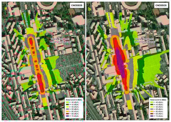
Figure 11.
Mapping the noise variations within traffic light intra-cycles. The figures show the averaged lower (a) and higher (b) noise level maps (two of the 110 possible) during the hour of simulation.
Note that Figure 8 and Figure 9 show second by second the variation of the noise measured by a virtual sound meter at 1.3 m high. With the same data from traffic microsimulation (and of course the same power emission levels) these maps were developed, but at 4 m high.
In addition to those 110 maps that show the dynamics of noise in the area with that traffic load, it is also possible to represent an average view of the equivalent noise throughout the simulation time (not represented in this paper), following the method widely tried, for example, see [31].
4. Analysis and Discussion
There are two tasks ahead. The first is to validate the DTNA tool and the second has to do with the possible implementation of the model as an analytical tool for the action plans. There are in the literature, some urban noise indicators well adapted to the traffic signals period [21,46,47]. These kinds of noise indicators are generally used to investigate the pattern of noise variations within inter-cycles and intra-cycles of traffic lights. The first involves finding the variability of noise analyzed cycle by cycle, averaging, and examining its evolution during the simulation and/or measurement time. The second analyzes the variability of noise second by second during the traffic light cycle, averaging the total number of cycles.
4.1. Validation of the Model Using Noise Variations within Inter-Cycles of Traffic Lights
The problem of analyzing the distribution represented in Figure 9 in contrast to Figure 7, is due to the problem of background noise. Once the anomalous sound events were removed from the measured series (some of them reach LAeq,T=1s = 102.9 dBA), which are due to ambulance sirens and high power motorcycles, the distribution shown in Figure 7 was obtained. It has an asymmetrical shape with two humps. This distribution shape allows understanding that there are at least two sources of noise in the area and that it has two mixed distributions. The first and most important source caused by the traffic on the avenue as it passes through the measuring point could be visually assigned at approximately 68 dBA. The second, the background noise, is the noise caused in the moments in which by different causes the main noise is turned off and loses importance. Then, not from other avenues and the Marasesti avenue itself but out of the limits of the 401 m analyzed, etc. This begins to stand out in special situations when there is no traffic in the area near the sound level meter, or, for example, when the traffic light is red, with the vehicles stopped.
Energetically subtracting the background noise from the series of “total” noise measurements is complicated precisely by their dispersion. In this case, there is an area in which the traffic noise mixes with the background noise, causing the subtraction to generate uncertainty in this decision area.
Several alternatives were estimated, some of which were assessed as more correct than others. Finally, the process used went through the following steps:
- Splitting both time series (simulated and real) into intervals of 110 s, which coincide with the red-green-yellow-red traffic signal cycle, in such a way that it extract both the LAeq, for each of the cycles (inter-cycles analysis).
- The cycle of the passage of the ambulance was eliminated from the real series measured, not only by the anomaly detected but because the traffic is altered, and the normal flow of vehicles is altered by the presence of the ambulance.
- It was added energetically to the simulated data series, 50 dBA, which corresponds to the lowest and prolonged LAeq level of background noise measured during the measurement period. This also eliminates the presence of zeros. Another possibility (not contemplated in this study) is to take into account only the green time in the analysis.
- Noise data is energetically averaged within each cycle.
The processing to which the data was subjected makes them a better estimator of noise caused by traffic and much more robust in the presence of background noise. In the new data series, the background noise is negligible energetically in comparison with the LAeq of the estimated traffic flow for each of these cycles. After processing the data, Figure 12 shows the distribution of the new series.
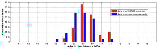
Figure 12.
Distribution of LAeq, T = 110 synchronized with the traffic light for both the simulated series (red) and the series measured (in blue) corrected for the anomalies.
A normality test was carried out and it can be said with 95% confidence that the distributions are not normal, so nonparametric tests were executed. The contrasts that are presented below allow checking if the two samples (measurement and simulation) come from the same population, through the analysis of their distributions. Some tests were performed using SPSS (Statistical Package for the Social Science) program: Mann–Whitney U test, Kolmogorov–Smirnov Z test, and Wald–Wolfowitz test. Considering that Ho is the null hypothesis whose formulation is “The two series are part of the same population and their distribution is identical”, this would be the evidence that the results of the simulation are representing acoustically what is happening on the Bacău’s Marasesti Avenue. A Kolmogorov–Smirnov test for two independent samples SPSS results is presented (Table 5).
Table 5.
Frequencies.
The Kolmogorov–Smirnov contrast provides the following results that show that there are no significant differences between the assigned scores since the level of significance corresponding to the value of the test statistic is 0.163 (Table 6).
Table 6.
Test statistics.
With a p-value (probability value of deviation) >0.1, Ho cannot be rejected. Therefore, it can be affirmed that both data series belong to the same process and it can be affirmed with a 95% level of significance that the simulated series perfectly predicts the results obtained directly from the environmental noise measurements. Mann–Whitney and Wald–Wolfowitz tests both for independent samples confirmed the result.
4.2. Dynamic Maps for Action Plans Using Noise Variations within Intra-Cycles of Traffic Lights
Selecting the three maps developed with CNOSSOS (Figure 10—map on the right (b) and Figure 11—both maps) the noise level pressure at 7.5 and 15 m from the centerline of the closest lane were selected. Figure 13 shows the results at the sampled points separated 20 m. Figure 13 presents that the dynamic tool gives much more precise information about noise space/time variability. The graph calculated from the difference in maps provides a clear idea of where the noise problem arises and how it evolves temporarily. This information helps to choose what is the most appropriate mitigation measures for the traffic noise management of the analyzed area.
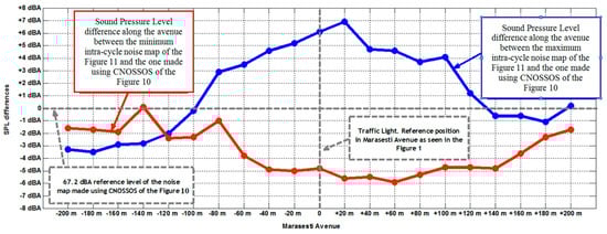
Figure 13.
Sound pressure level difference along the Marasesti Avenue between the maximum (in blue) and minimum (in red) intra-cycle noise maps with respect to the noise map carried out with the averaged traffic data for the measurement interval and without the presence of the traffic light.
5. Multifractal Model
As previously discussed, micro-simulation traffic models focus on each participating vehicle whose position, speed, and acceleration are considered in time, second by second. Dynamic Traffic Noise Assessment Tool (DTNA) was used to develop noise maps that show variation in traffic noise, avoiding a static description of this noise. Obviously, the generated noise in these conditions is a space/time function in terms of acoustic power from every vehicle in that street. It is not an easy task to precisely evaluate, and predict, the traffic noise, which must be separated from background noise. The uncertainty amount, large numbers of variables involves, the dynamic character of the DTNA tool leads us to the idea to try a theoretical approach of multifractal type. Consequently, accepting the nondifferentiable behavior in the study of the acoustic field, the approximation of acoustic waves of multifractal type is detailed below.
5.1. From Differentiability to Nondifferentiability in a Hydrodynamic Approach
Known models, for example hydrodynamic-type models; kinetic-type models [48,49,50] used to describe complex fluid dynamics (compressible and incompressible complex fluids) are based on the uncertain hypothesis that the variables describing them are differentiable. The success of these models must be understood gradually in domains in which differentiability is still valid. However, the differential procedures are not suitable when describing processes related to complex fluid dynamics, which imply nonlinearity and chaos (for example acoustic dynamics in complex fluids—it is reminded that this is the de-facto case [51,52]). Since the nondifferentiability appears as a universal property of the complex fluids [50,51,52,53,54], it is necessary to construct nondifferentiable physics of complex fluids. In such a conjecture, by considering that the complexity of the interaction process is replaced by nondifferentiability, it is no longer necessary to use the entire classical “arsenal” of quantities from the standard physics of fluids (differentiable physics of fluids). Therefore, in order to describe complex fluid dynamics by remaining faithful to the differentiable mathematical procedures, it is necessary to employ a multifractal paradigm, which explicitly introduces scale resolutions, both in the expression of the variables and in the fundamental equations which govern complex fluid dynamics. This means that, instead of “working” with a single variable described by a strict nondifferentiable function, it is possible to “work” only with approximations of this mathematical function, obtained by averaging them on different scale resolutions. As a consequence, any variable purposed to describe complex fluid dynamics will perform as the limit of a family of mathematical functions, this being nondifferentiable for null scale resolutions and differentiable otherwise [53,54,55,56].
In such a context, the dynamics of any complex fluid structural units become operational in the multifractal paradigm through the Multifractal Theory of Motion [54,55,56,57]. In this theory, the dynamics of any structural units of the complex fluids are described through multifractal curves, which “manifest” themselves like multifractal Schrodinger type geodesics or like multifractal hydrodynamic type geodesics on multifractal manifolds. In the following we will analyze the acoustic dynamics in a complex fluid by using the following multifractal hydrodynamic framework [55,56]:
with Q the specific multifractal potential:
and
In Equations (3)–(6) the specific multifractal potential, Equation (5), is a measure of the movement curves “breaking”, is the differentiable velocity of the complex fluid independent of the resolution scale dt, is the state density of multifractal type, xl is the spatial coordinate of multifractal type, t is the temporal coordinate of a non-multifractal type which is also an affine parameter of the movement curves, is a parameter associated with the multifractal–non-multifractal scale transitions, is the singularity spectra of order of the multifractal dimension DF and is the singularity index of the multifractal dimension [53,57,58]. Moreover, Equation (3) corresponds to the multifractal conservation law of specific momentum and Equation (4) corresponds to the multifractal conservation law of state density.
There are many modes, and thus a varied selection of definitions of multifractal dimensions, the multifractal dimension in the sense of Kolmogorov, the multifractal dimension in the sense of Hausdorff-Besikovich [53,57,58], etc. Selecting one of these definitions and operating in the complex fluid dynamics, the value of the multifractal dimension must be constant and arbitrary for the entirety of the dynamical analysis. For example, it is regularly found DF < 2 for correlative processes, DF > 2 for noncorrelative processes etc. In such a conjecture, operating with the singularity spectrum f(α) it is possible to identify not only the “areas” of the complex fluid dynamics that are characterized by a certain multifractal dimension, but also the number of “areas” whose multifractal dimensions are situated in an interval of values. Moreover, through f(α) it is possible to identify classes of universality in the complex fluid dynamics laws, even when regular or strange attractors have different aspects [57,58].
For the case in which the complex fluid suffers an external constrains of type, where p is the pressure, the hydrodynamic equations of the multifractal type become [55,56]:
5.2. Acoustic Waves Approximation of Multifractal Type
The approximation of acoustic waves of multifractal type implies the functionality of the following relations:
where the index “0” specify the initial values, the index “,” the perturbed values, and the velocity of the acoustic wave in the complex fluid. By operating with these relations in Equations (7) and (8), and using the procedure from [48], we obtain the propagation equation of the acoustic waves of multifractal type:
where is the Laplace operator of the first order and is the Laplace operator of the second order.
Assuming for a space–time dependence (z,t):
where is the amplitude, k is the acoustic wave number, and is the pulsation of the acoustic wave, then the dispersion relation associated to (10) becomes:
Moreover, defining the following parameters:
(i) the pulsation of the differentiable component of the acoustic wave of multifractal type ()
(ii) the pulsation of the nondifferentiable component of the acoustic wave of multifractal type ()
(iii) velocity of the nondifferentiable (multifractal) component of the acoustic wave of multifractal type (),
(iv) the velocity of the differentiable–nondifferentiable component of an acoustic wave of multifractal (c)
the Equation (12) takes the equivalent forms:
From here, it results the phase velocity of an acoustic wave of multifractal type:
and the group velocity of an acoustic wave of multifractal type:
respectively:
Therefore, for , or in pulsation terms , in the complex fluid there is an acoustic wave of multifractal type propagating with a phase velocity of multifractal type, Equation (18), and a group velocity of multifractal type, Equation (19). The product of these velocities satisfies the De Broglie type relation either as at a differentiable scale resolution or at a nondifferentiable scale resolution. However, if , or in pulsation terms , in the complex fluid there is a damped acoustic wave of multifractal type, which stops at:
A particular situation can be found when , or in pulsation term . Then, defining the acoustic refractive index of multifractal type:
the above-mentioned restriction implies an infinite value for . Therefore, “exotic states” of matter are mimicked in the complex fluid which implies the existence of some special topologies, such as “Acoustic Black Hole” of multifractal type. In particular, for movements of the complex fluid’s structural units on Peano type curves at Compton scale resolution (i.e., for DF = 2, and , where h is the Planck constant and m0 is the rest mass of the complex fluid structural units) the generating condition of “Acoustic Black Hole” implies:
while for similar movements at a mesoscale:
where D is the diffusion coefficient of the complex fluid particles [54]. We would like to present in Table 7, some collapse length characteristics for complex fluids at various scale resolutions:
Table 7.
Acoustic collapse length for fluid complex at various scale resolutions.
It results that if the minima relevant dimensions of any complex fluid structural units are increasing the acoustic collapse length decreases, regardless of the scale resolution.
5.3. Pulsation–Velocity Correlation through Patches of Riemann Type
The dispersion Equation (12) can be rewritten according to Equation (17) as:
and allows, both in the pulsation space as well as in velocity space, the development of Cayley–Klein absolute geometries for the characterization of the propagation process parameters variation of an acoustic wave of multifractal type.
In the most general case, the metric of the Lobachevsky plan can be provided as a Caylean metric of a Euclidian plan for which the absoluteness is the circle with the unit radius:
This way, the Lobachevsky plane can be put into biunivocal correspondence with the interior of this circle. The general procedure of metrization of Caylean space starts with the definition of the metric as an an-harmonic ratio. With this purpose, let us suppose that the absoluteness of the space is represented by the quadradic form Ω (X, Y), where X denotes any vector.
The Caylean metric is given by the differential quadratic form [59,60,61,62]:
where Ω (X,Y) is the duplication of Ω (X,X) and f is a constant connected to the space curvature.
In the case of the Lobachevsky plane, we have:
which yields:
Performing now the coordinate transformations:
where is the complex conjugate of h, the metric (29) becomes:
As easily seen, the absoluteness goes to the straight line Im h = 0, while straight lines of the Euclidian plane go to circles with the centers on the real axis of the complex plane (h). The metric (31) is invariant with respect to a group of transformations whose explicit form will be given as follows. For this purpose, let us consider the real homographic transformation on the variable h [59,60,61,62].
The conjugates of these two complex quantities h and h’ are connected, obviously, by the same transformation:
Transformations (32) and (33) form a group of two variables with three parameters (one of the quantities a, b, c, d is not essential), as it can easily be verified. Since:
it immediately yields:
The structure of this group is typical of a SL(2R), which we take in the standard form:
where are the infinitesimal generators of the group:
Now, considering the previous results (25), both the pulsation space and the velocity space it can be structured in an absolute geometry as varieties of Riemann type on Poincare metrics:
for the pulsation space, respectively:
for the velocity space.
The metrics (38) and (39) are invariant with respect to two groups of SL(2R) type whose infinitesimal operators:
for pulsation space, respectively:
for the velocities space, satisfy the algebras:
and
Now, we can describe the topography of an acoustic wave of multifractal type through relations between the pulsation and velocity, one characterized by and its complex conjugate, the other characterized by and its complex conjugate. Their correlation is universal [60,61,62], i.e., scale-invariant, in the sense defined above. Following this, each one of the two quantities is described by the operators (40) and (41) and their properties of correlation are to be defined in terms of the joint invariant functions of the Stoka system [63].
The Stoka system [63] for operators (40) and (41) describing the propagation of the acoustic wave in complex fluids and their correspondents are:
Notice that the system has the rank 3, so there is only one independent integral. This is the cross-ratio of the following form:
where is real and we took the square in order to account for the fact that the cross-ratio (45) is always positive. Any joint invariant function is here a regular function of this cross-ratio. As the values of the cross-section (45) are always positive, we can assume them smaller than unity in absolute value, making thus legitimate the notation , where Ψ is arbitrary. Then the variable is by Equation (45) related to through the linear relation [54,55,56].
where we take , provided is given by the equation:
with
The basic variable in Equation (45) is then given in (47).
6. Model Results Analysis
Through this approach, the topography of an acoustic wave is argued by the relations between the pulsation and velocity of the sound wave. Their correlation is scale-invariant. A connection can be made between the representative hyperbolic geometry of the acoustic wave propagation problem and the physical space regions occupied by the “physical object” involved in this problem. This rather unusual approach has never been used before and has the advantage of being developed in abstract multifractal space and it can generate a wide range of acoustic waves. Modeling traffic acoustic waves can be rather difficult, as it not only has to be related to the source but also to the multiple overlap with noise and other acoustic waves. The novelty of our approach also comes from the freedom that the multifractal model presents through the fractality degree of each acoustic wave, the scale resolution chosen to generate and observe the time-series and the control parameter(s) that have the role to simulate external constraints existing in real noise acoustic waves.
The theoretical model built in a multifractal paradigm leads to the finding of relation for the acoustic field amplitude in Equation (47). By plotting the real component () of the time series of the acoustic field amplitude it can be generated for specific scale resolutions ( Ωt, with Ω the normalized scale resolution and t the normalized time) and control parameter () (they will characterize unique acoustic waves generated for particular sound sources). In Figure 14a,b it can be seen oscillatory dynamics of acoustic wave time-series. The period-doubling signature can be seen throughout the simulated acoustic wave time series at each scale resolution: Ω = 7.8 (a) and Ω = 9.7 (b). It was also observed a modulated periodical scenario useful for acoustic wave dynamics and possible intermittence scenarios depending on the control parameter (r) and the scale resolution. The multifractal model encompasses various scenarios for the acoustic wave time-series which can help to understand more complicate real data which are a combination of various types of acoustic waves mixed in a rather complex manner. However, it is worth noting that these time-series are describing the evolution of the acoustic wave generated by singular signals evolving in a multifractal medium.
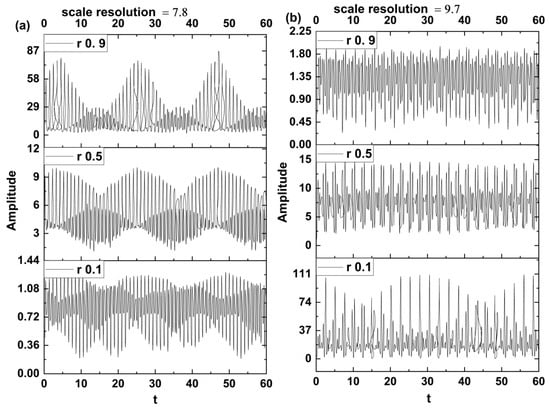
Figure 14.
Time-series of for different values of and : (a) ; (b) .
Furthermore, using the multifractal model paradigm, certain behaviors of acoustic waves can be generated at a particular scale resolution for one fractality degree. However, in reality, the empirical data contains contributions from several such subsystems which are combined and have a weighted contribution to the overall signal. In Figure 15, two signals generated and unified through the contributions of multifractal systems with various scale resolutions (7.8, 8.8, and 10) in a superposition scenario (a) and a polynomial type mixing scenario in (b) are shown. Both approaches are encompassing a similar conclusion. Out of the multitude of signals interacting and creating the acoustic fractal medium there are some of them that can be considered driving forces in shaping the real recorded signal. This can be seen in Figure 15 where we notice a modulation of the signal obtained via superposition scenario which means that the acoustic signal generated at low scale resolutions and low fractality degrees can modulate high fractality signals. It can be appreciated that both models are promising and can be used at a starting point for further development of the model.
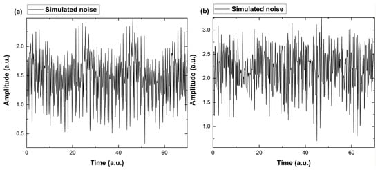
Figure 15.
Simulated noise generate by combinatorial mixing of single-fractal systems from the multifractal theoretical model by superposition of signals (a) and polynomial mixing (b).
7. Conclusions
Traffic microsimulation models are very useful to judge urban noise as they allow a deep knowledge of its causes, and therefore they provide a very powerful tool for the analysis of the proposed action plans against the noise. The local factors of each country must be validated before being introduced in the VISSIM traffic model, as their importance is much higher than other local factors of the vehicle fleet that can be included in the CNOSSOS-EU road noise emission model (such as the age of the vehicle fleet). Therefore, aspects such as the level of aggressiveness of the drivers, the response time, the safety distance between vehicles, the behavior to overtake vehicles, and above all the cruise speed (desired) are very important to transfer the results of the models from one country to another.
Considering the statistical analysis it can be affirmed with a confidence level of 95% that once the traffic model in VISSIM was calibrated for the studied medium-sized city in the actual conditions of the avenue during the test time, the environmental noise measurements LAeq of the total traffic which passes through the avenue and the simulated noise data LAeq of the total traffic of the same avenue generated with the dynamic traffic noise simulation method, are equal. The validation of the dynamic traffic noise assessment tool shows that this traffic noise prediction method is suitable for the evaluation of action plan effectiveness against urban noise, and specifically, this has been proven for the city of Bacau when cars use summer tires. The mathematical model was developed based on Cayley–Klein-type absolute geometries that implied harmonic mappings between the usual space and the Lobacevsky plane in a Poincaré metric. This allowed studying the isomorphism of two groups of SL(2R) type, and through Stoka formalism showcased joint invariant functions that allow associations of pulsations–velocities manifolds type. Based on the complexity of our model and its multitude of degrees of freedom, the multifractal approach can be used through the fractality degree of each acoustic wave to simulate external constraints that can be found in real ones. Therefore, the multifractal approach of acoustic waves propagation and their sources in the traffic area offers another perspective of traffic noise interpretation and simulation.
Author Contributions
Conceptualization, J.L.C., M.A. and C.B.; software, J.L.C, E.N. and F.N. validation, R.H. and C.B.; formal analysis, A.P., J.L.C. and S.A.I.; investigation, V.N. and M.A.; writing—original draft preparation, A.P.; S.A.I. and C.B. writing—review and editing, R.H.; visualization, F.N. and S.A.I.; supervision, M.A. and V.N.; All authors have read and agreed to the published version of the manuscript.
Funding
This research received no external funding.
Conflicts of Interest
The authors declare no conflict of interest.
References
- European Environment Agency. Population Exposure to Environmental Noise. Available online: https://www.eea.europa.eu/data-and-maps/daviz/number-of-people-exposed-to-6#tab-googlechartid_chart_21Nov2018 (accessed on 1 October 2019).
- European Environmental Agency. Country Fact Sheets: Romania. Noise in Europe 2017 Overview of Policy-Related Data; European Environmental Agency: Bruxelles, Belgium, 2017. [Google Scholar]
- Griefahn, B.; Basner, M. Disturbances of sleep by noise. In Proceedings of the Acoustics, Gold Coast, Australia, 2–4 November 2011. [Google Scholar]
- Meijker, H.; Knipschild, P.; Sallé, H. Road traffic noise annoyance in Amsterdam. Int. Arch. Occup. Environ. Health 1985, 56, 285–297. [Google Scholar] [CrossRef]
- Méline, J.; Van Hulst, A.; Thomas, F.; Karusisi, N.; Chais, B. Transportation noise and annoyance related to road traffic in the French RECORD study. Int. J. Health Geogr. 2013, 12, 44. [Google Scholar] [CrossRef] [PubMed]
- Muzet, A. Environmental noise, sleep and health. Sleep Med. Rev. 2007, 11, 135–142. [Google Scholar] [CrossRef] [PubMed]
- Okokon, E.; Turunen, A.; Ung-Lanki, S.; Vartainen, A.K.; Tiittanen, P.; Lanki, T. Road-traffic noise: Annoyance, risk perception, and noise sensitivity in the finnish adult population. Int. J. Env. Res. Public Health 2015, 12, 5712–5734. [Google Scholar] [CrossRef] [PubMed]
- Chetoni, M.; Ascari, E.; Bianco, F.; Fredianelli, L.; Licitra, G.; Cori, L. Global noise score indicator for classroom evaluation of acoustic performances in Life Gioconda project. Noise Mapp. 2016, 3, 157–171. [Google Scholar] [CrossRef]
- Babisch, W. Cardiovascular effects of noise. Noise Health 2011, 13, 201–204. [Google Scholar] [CrossRef]
- Stansfeld, S.A.; Haines, M.M.; Burr, M.; Berry, B.; Lercher, P. A review of environmental noise and mental health. Noise Health 2000, 2, 1–8. [Google Scholar]
- Stansfeld, S.A.; Matheson, M.P. Noise pollution: Non-auditory effects on health. Br. Med. Bull. 2003, 68, 243–257. [Google Scholar] [CrossRef]
- Sørensen, M.; Andersen, Z.J.; Nordsborg, R.B.; Becker, T.; Tjønneland, A.; Overvad, K.; Nielsen, O.R. Long-term exposure to road traffic noise and incident diabetes: A cohort study. Environ. Health Persp. 2013, 121, 217–222. [Google Scholar] [CrossRef]
- Directive 2002/49/EC of the European Parliament and of the Council of 25 June 2002 Relating to the Assessment and Management of Environmental Noise. Available online: https://eur-lex.europa.eu/legal-content/EN/TXT/?uri=CELEX%3A32002L0049 (accessed on 1 June 2019).
- Institutul de Cercetări în Transporturi—Incertrans SA. Elaborarea Hartilor de Zgomot si a Planurilor de Actiune Pentru Municipiul Bacau. In Etapa 3: Informatii Necesare Actualizarii Planului de Reducere a Zgomotului Pentru Municipiul Bacau—Raport Final; Institutul de Cercetări în Transporturi—Incertrans SA: Bacau, Romania, 2018. [Google Scholar]
- European Commission. Commission Directive (EU) 2020/367 Amending Annex III to Directive 2002/49/EC of the European Parliament, and of the Council as Regards the Establishment of Assessment Methods for Harmful Effects of Environmental Noise; European Commission: Bruxelles, Belgium, 2020. [Google Scholar]
- Miedema, H.M.; Oudshoorn, C.G. Annoyance from transportation noise: Relationships with exposure metrics DNL and DENL and their confidence intervals. Environ. Health Persp. 2013, 109, 409–416. [Google Scholar] [CrossRef]
- Basner, M.; McGuire, S. WHO environmental noise guidelines for the European region: A systematic review on environmental noise and effects on sleep. Environ. Res. Public Health 2018, 15, 519. [Google Scholar] [CrossRef] [PubMed]
- Caniato, M.; Bettarello, F.; Schmid, C.; Fausti, P. Assessment criterion for indoor noise disturbance in the presence of low frequency sources. Appl. Acoust. 2016, 113, 22–33. [Google Scholar] [CrossRef]
- Mirowska, M.J. Evaluation of low-frequency noise in dwellings. New Polish recommendations. J. Low Freq. Noise Vib. Act. Control 2001, 20, 69–74. [Google Scholar] [CrossRef]
- Ascari, E.; Licitra, G.; Teti, L.; Cerchiai, M. Low frequency noise impact from road traffic according to different noise prediction methods. Sci. Total Environ. 2015, 505, 658–669. [Google Scholar] [CrossRef] [PubMed]
- Can, A.; Aumond, P.; Michel, S.; de Coensel, B.; Ribeiro, C.; Botteldooren, D.; Lavandier, C. Comparison of noise indicators in an urban context, Inter-Noise. In Proceedings of the 45th International Congress and Exposition of Noise Control Engineering, Hamburg, Germany, 21–24 August 2016. [Google Scholar]
- De Coensel, B.; Botteldooren, D.; De Muer, T.; Berglund, B.; Nilsson, M.E.; Lercher, P. A model for the perception of environmental sound based on notice-events. J. Acoust. Soc. Am. 2009, 126, 656–665. [Google Scholar] [CrossRef]
- Sato, T.; Yano, T.; Björkman, M.; Rylander, R. Road traffic noise annoyance in relation to average noise level, number of events and maximum noise level. J. Sound Vib. 1999, 223, 775–784. [Google Scholar] [CrossRef]
- Brown, A.L. An overview of concepts and past findings on noise events and human response to surface transport noise. In Proceedings of the 43rd Nternational Congress and Exposition on Noise Control Engineering (Internoise), Melbourne, Australia, 16–19 November 2014. [Google Scholar]
- Chevallier, E.; Can, A.; Nadji, M.; Leclercq, L. Improving noise assessment at intersections by modeling traffic dynamics. Transport. Res. Part D Transp. Environ. 2009, 14, 100–110. [Google Scholar] [CrossRef]
- De Coensel, B.; Botteldooren, D.; Vanhove, F.; Logghe, S. Microsimulation based corrections on the road traffic noise emission near intersections. Acta Acust. United Acust. 2007, 93, 241–252. [Google Scholar]
- De Coensel, B.; Can, A.; Degraeuwe, B.; De Vlieger, I.; Botteldooren, D. Effects of traffic signal coordination on noise and air pollutant emissions. Environ. Model. Softw. 2012, 35, 74–83. [Google Scholar] [CrossRef]
- De Coensel, B.; Brown, A.L.; Bottledooren, D. Modelling road traffic noise using distributions for vehicle sound power level. In Proceedings of the 41st International Congress and Exposition on Noise Control Engineering (Inter-Noise-2012), New York, NY, USA, 19–22 August 2012. [Google Scholar]
- Estévez-Mauriz, L.; Forssén, J. Dynamic traffic noise assessment tool: A comparative study between a roundabout and a signalised intersection. Appl. Acoust. 2017, 130, 71–86. [Google Scholar] [CrossRef]
- Feng, L.; Yushan, L.; Ming, C.; Du, C. Dynamic simulation and characteristics analysis of traffic noise at roundabout and signalized intersections. Appl. Acoust. 2014, 121, 14–24. [Google Scholar]
- Cueto, J.L.; Petrovici, A.M.; Hernández, R.; Fernández, F. Analysis of the impact of bus signal priority on urban noise. Acta Acust. United Acust. 2017, 103, 561–573. [Google Scholar] [CrossRef]
- Petrovici, A.M.; Cueto, J.L.; Hernandez, R.; Nedeff, V. Smart mobility strategies based on bus signal priority for noise reduction. In Proceedings of the Congress publication, Euroregio/Tecniacustica’16, Oporto, Portugal, 13–15 June 2016. [Google Scholar]
- Petrovici, A.M.; Cueto, J.L.; Hernandez, R.; Marquez, S.D.; Lerida, S.D. Effects upon urban noise of the prioritization of buses at intersections. In Proceedings of the Congreso Tecniacustica, Valencia, Portugal, 21–23 October 2015. [Google Scholar]
- Petrovici, A.M. Traffic Microsimulation as a Tool in the Development of Action Plans against Noise in Urban Areas. Ph.D. Thesis, Vasile Alecsandri University of Bacau, Bacau, Romania, 2018. [Google Scholar]
- Kephalopoulos, S.; Paviotti, M.; Anfosso-Lédée, F. Common Noise Assessment Methods in Europe (CNOSSOS-EU); Publications Office of the European Union: Luxembourg, 2012. [Google Scholar]
- Jonasson, H. Test method for the entire vehicle. HAR11TR-020301-SP10, Harmonoise Project, Report. Tech. Rep. 2004. [Google Scholar]
- Harmonoise, HAR11TR-020614-SP09v4, Source modelling of road vehicles. 2004.
- Imagine: The Noise Emission Model For European Road Traffic. IMA55TR-060821-MP10 P10. 2007. Available online: http://www.imagine-project.org/ (accessed on 1 October 2019).
- Peeters, B.; van Blokland, G. Correcting the CNOSSOS-EU road noise emission values. In Proceedings of the Euronoise 2018—Conference, Hersonissos, Greece, 27–31 May 2018. [Google Scholar]
- De Leon, G.; Fidecaro, F.; Cerchiai, M.; Reggiani, M.; Ascari, E.; Licitra, G. Implementation of CNOSSOS-EU method for road noise in Italy. In Proceedings of the 23rd International Congress on Acoustics, Aachen, Germany, 9–13 September 2019. [Google Scholar]
- Fellendorf, M. A microscopic simulation tool to evaluate actuated signal control including bus priority. Technical papers, Session 32. In Proceedings of the 64th ITE Annual Meeting, Dallas, TX, USA, 16–19 October 1994. [Google Scholar]
- Zhang, J. Evaluating the Environmental Impacts of Bus Priority Strategies at Traffic Signals. Ph.D. Thesis, University of Southampton, Faculty of Engineering and the Environment, Southampton, UK, 2011. [Google Scholar]
- Brown, A.L.; Tomerini, D. Distribution of the noise level maxima from the pass-by of vehicles in urban road traffic streams. Road Transp. Res. 2011, 20, 41. [Google Scholar]
- Garg, N.; Maji, S. A critical review of principal traffic noise models: Strategies and implications. Environ. Impact Assess. Rev. 2014, 46, 68–81. [Google Scholar] [CrossRef]
- De Coensel, B.; Brown, A.L.; Tomerini, D. A road traffic noise pattern simulation model that includes distributions of vehicle sound power levels. Appl. Acoust. 2016, 111, 170–178. [Google Scholar] [CrossRef]
- Can, A.; Leclercq, L.; Lelong, J.; Defrance, J. Capturing urban traffic noise dynamics through relevant descriptors. Appl. Acoust. 2008, 69, 1270–1280. [Google Scholar] [CrossRef]
- Can, A.; Leclercq, L.; Lelong, J.; Botteldooren, D. Traffic noise spectrum analysis: Dynamic modeling vs. Experimental observations. Appl. Acoust. 2010, 71, 764–770. [Google Scholar] [CrossRef]
- Luis, G. Complex Fluids; Springer: Barcelona, Spain, 1993. [Google Scholar]
- Badii, R. Complexity: Hierarchical Structures and Scaling in Physics; Cambridge University Press: Cambridge, UK, 1997. [Google Scholar]
- Mitchell, M. Complexity: A Guided Tour; Oxford University Press: New York, NY, USA, 2009. [Google Scholar]
- Yam, B.Y. Dynamics of Complex Systems; Taylor and Francis: New York, NY, USA, 1999. [Google Scholar]
- Deville, M.; Gatski, B.T. Mathematical Modeling for Complex Fluids and Flows; Springer: Berlin, Germany, 2012. [Google Scholar]
- Mandelbrot, B.B. The Fractal Geometry of Nature; W. H. Freeman and Co.: San Francisco, CA, USA, 1982. [Google Scholar]
- Nottale, L. Scale Relativity and Fractal Space-Time: A New Approach to Unifying Relativity and Quantum Mechanics; Imperial College Press: London, UK, 2011. [Google Scholar]
- Merches, I.; Agop, M. Differentiability and Fractality in Dynamics of Physical Systems; World Scientific: Hackensack, NJ, USA, 2016. [Google Scholar]
- Agop, M.; Paun, V.P. On the new perspectives of fractal theory. Fundaments and Applications; Romanian Academy Publishing House: Bucharest, Romania, 2017. [Google Scholar]
- Jackson, E.A. Perspectives of Nonlinear Dynamics; Cambridge University Press: New York, NY, USA, 1993. [Google Scholar]
- Cristescu, C.P. Nonlinear dynamics and chaos.Theoretical Fundaments and Applications; Romanian Academy Publishing House: Bucharest, Romania, 2008. [Google Scholar]
- Mazilu, N.; Agop, M. At the Crossroads of Theories. Between Newton and Einstein—The Barbilian Universe; ArsLonga Publishing House: Iasi, Romania, 2010. [Google Scholar]
- Agop, M.; Merches, I. Operational Procedures Describing Physical Systems; CRC Press, Taylor & Francis Group: Boca Raton, FL, USA, 2019. [Google Scholar]
- Mazilu, N.; Agop, M. Skyrmions. A Great Finishing Touch to Classical Newtonian Philosophy; World Philosophy Series; Nova Science Publishers: New York, NY, USA, 2012. [Google Scholar]
- Bujoreanu, C.; Irimiciuc, S.; Benchea, M.; Agop, M. A fractal approach of the sound absorption behaviour of materials. Theoretical and experimental aspects. Int. J. Non-Linear Mech. 2018, 103, 128–137. [Google Scholar] [CrossRef]
- Stoka, M.I. Integral Geometry; Romanian Academy Publishing House: Bucharest, Romania, 1967. [Google Scholar]
Publisher’s Note: MDPI stays neutral with regard to jurisdictional claims in published maps and institutional affiliations. |
© 2020 by the authors. Licensee MDPI, Basel, Switzerland. This article is an open access article distributed under the terms and conditions of the Creative Commons Attribution (CC BY) license (http://creativecommons.org/licenses/by/4.0/).