Abstract
Radiative transfer (RT) in spectral lines in plasmas and gases under complete redistribution of the photon frequency in the emission-absorption act is known as a superdiffusion transport characterized by the irreducibility of the integral (in the space coordinates) equation for the atomic excitation density to a diffusion-type differential equation. The dominant role of distant rare flights (Lévy flights, introduced by Mandelbrot for trajectories generated by the Lévy stable distribution) is well known and is used to construct approximate analytic solutions in the theory of stationary RT (the escape probability method is the best example). In the theory of nonstationary RT, progress based on similar principles has been made recently. This includes approximate self-similar solutions for the Green’s function (i) at an infinite velocity of carriers (no retardation effects) to cover the Biberman–Holstein equation for various spectral line shapes; (ii) for a finite fixed velocity of carriers to cover a wide class of superdiffusion equations dominated by Lévy walks with rests; (iii) verification of the accuracy of above solutions by comparison with direct numerical solutions obtained using distributed computing. The article provides an overview of the above results with an emphasis on the role of distant rare flights in the discovery of nonstationary self-similar solutions.
1. Introduction
Self-similarity in the theory of transport phenomena means that the space-time evolution of the Green’s function, which by definition corresponds to the solution of a transport equation with an instant point source, is described for transport on a uniform background by a function of a single variable. For ordinary diffusion, i.e., Brownian motion described by a Fokker–Planck differential equation with the diffusion coefficient D, the argument of the Green function, which is a Gaussian, determines the scaling law for the propagation front rfr(t) ~ (Dt)1/2.
For non-Brownian transport with a long-tailed, power-law probability density function (PDF) for the carrier’s step-length distribution, the transport is a superdiffusive one (see, e.g., [1,2,3,4,5,6,7]) because the exponent in the time dependence of the propagation front exceeds its diffusion value of 1/2. Here, the long-free-path trajectories of the carriers (named by B. Mandelbrot [8], Lévy flights, cf. page IX in Reference [1]) provide the dominant contribution to the Green’s function. The case of the Lévy flights-based transport should be extended when one has to take into account the finite velocity of the carriers of the medium’s perturbation. This case is named Lévy walk + rests (see Figure 1 in [7]) and corresponds to allowing for the retardation effects in the Lévy flights. The alternative name for superdiffusive transport is nonlocal transport. The term nonlocal corresponds to the fact that the transport equation is such an integral, in space variables, equation, which can not be reduced to a differential one. For all types of superdiffusive/nonlocal transport, the step-length PDF has a divergent second and all higher moments. Therefore, the measurements of the step-length PDF can not be used for interpreting the experimental data for the propagation front of the Green’s function.
One of the most developed examples of superdiffusive/nonlocal transport is the radiative transfer in the spectral lines of atoms and ions in gases and plasmas. The respective transport equation for the space-time evolution of the density of excited atoms/ions is known as the Biberman–Holstein equation [9,10,11]. This equation is derived from the system of differential kinetic equations for photons and atoms or ions. The Biberman–Holstein model is valid for the complete redistribution (CRD) over photon frequency (within spectral line width) in the elementary act of the resonance scattering (i.e., absorption and subsequent emission) of the photon by an atom/ion. The CRD model corresponds to a Markovian process with the loss of memory by the photon during its trapping by the atom/ion. Already at the early stage of the studies with the Biberman–Holstein equation, it was realized (see, e.g., [12,13,14,15,16]) that the expansion/simplification of the integral term gives the diffusion coefficient, which explicitly depends on the size, L, of a finite medium and tends to infinity with L → ∞. Therefore, the very concept of diffusivity is inapplicable to this type of transport (it is curious that the term diffusion is sometimes applied to such phenomena). The propagation front should be defined in a way relevant to superdiffusion [12] (see also [11,16]) because, in an infinite medium, the respective mean squared displacement determined by the moment of the step-length PDF also diverges. The dominant contribution of the photons, emitted in the far wings of the spectral line shape where the photon’s free path is long, has been recognized in [13,14,15]. This feature of the Biberman–Holstein transport became the basis of the escape probability (EP) approaches [17,18,19].
The Biberman–Holstein model of radiative transfer in spectral lines of atoms and ions in plasma and gases was extended to the case of energy transfer in continuous spectra. This includes the following problems: the transfer of photorecombination radiation, which is also called the radiative transfer in the ionization continuum [20]; the nonlocal nonstationary heat transport by the plasma waves in hot plasmas, specifically by the longitudinal (electron Bernstein) waves [21] (this method extended the nonlocal transport model described by an integral equation in the case of the steady-state transport of heat by plasma waves (electron and ion Bernstein waves) [22] to the case of nonstationary transport); extension of the escape probability method for describing the energy loss due to the emission and absorption of plasma waves [23,24,25] (this method extended and modified the approach to the transport by electron cyclotron waves in toroidal magnetized plasmas in nuclear fusion systems) [26,27,28]. The application of the method [12] for the Green’s function of excited atoms in an infinite space to the case of a semi-infinite space was elaborated in [29,30]. The Biberman–Holstein model originally developed for gases and plasmas appears to be applicable to condensed media: the transfer of an excitation by resonance phonons in ruby [31] and the transfer of holes in an n-type semiconductor associated with the absorption of photons [32,33] are described by similar equations. We do not find the term Lévy flights in [9,10,11,12,13,14,15,16,17,18,19,20,21,22,23,24,25,26,27,28,29,30,31]; however, the type of transport in these papers refers precisely to Lévy flights-based transport.
In the theory of radiative transfer in astrophysics, the situation differs from that in the laboratory one: the above-mentioned system of differential kinetic equations for photons and atoms/ions is reduced to an integral, in space variables, equation for the radiation intensity (cf., e.g., [34,35]). Here, too, the dominant contribution of Lévy flights is recognized, however, as a rule without specifying their name.
The status of Lévy flight in the literature seems to be ambiguous. On the one hand, in the article “A Lévy flight for light” [36], it was stated that “…to date, it has not seemed possible to observe and study Lévy transport in actual materials. For example, experimental work on heat, sound, and light diffusion is generally limited to normal, Brownian, diffusion.” On the other hand, the dominant role of Lévy flight in the radiative transfer in spectral lines is recognized, e.g., in Reference [37] for the case of resonant radiation transfer in a Doppler-broadened hot atomic vapor: the experiments proved the theoretical conclusion [38] that the photon trajectories in the Biberman–Holstein model for Doppler, Lorentz, and Voigt spectral line shapes correspond to the Lévy flight-based transport.
An alternative way to treat the transport equation with integral over-spatial variables was developed in the form of fractional-order derivatives (see, e.g., [1,2,39,40]). In this formalism, it is easier to derive the scaling laws and, accordingly, the self-similar variables of possible solutions. However, obtaining an exact solution is often as difficult as in the formalism of the integral equation.
In the present paper, we provide a survey of the progress in the theory of nonstationary radiative transfer in spectral lines in plasmas and gases, achieved due to the elaboration of a method of deriving an approximate analytic self-similar solution for a wide class of nonstationary superdiffusive transport on a uniform background in the framework of integral equation formalism [41,42,43,44,45,46,47,48,49,50]. The method allows obtaining an approximate self-similar solution that is based on the following three building blocks, namely, scaling law for the propagation front, defined in a way relevant to superdiffusion, and asymptotics of the Green’s function far beyond and far in advance of the propagation front. All these characteristics are determined by Lévy flights, in the case of infinite velocity of medium’s perturbation carriers, or Lévy walks, in the case of a finite fixed velocity of the carriers. The high accuracy of the suggested self-similar solution in a broad range of variables of the problem is proved by comparing with numerical solutions of transport equations.
2. Materials and Methods
We start with the case of an infinite velocity of carriers (), which is associated with the case of Lévy flights (see, e.g., [1,7]), and continue with the case of a finite constant velocity of carriers (), which is associated with the case of Lévy walks (more precisely, Lévy walks with rests, see Figure 1 in [7]).
2.1. Approximate Self-Similar Solution of the Biberman–Holstein (BH) Equation (BH Step-Length PDF, , 3D Case)
2.1.1. Biberman–Holstein Equation and Its General Solution
The Biberman–Holstein equation [9,10,11] for radiative transfer in the spectral lines of atoms and ions in gases and plasmas describes the space-time evolution of the density of excited atoms/ions. This equation is derived from a system of equations for spatial density of excited atoms, f(r, t), and spectral intensity of resonance radiation. This system is reduced to a single equation for f(r, t), which turns out to be an integral equation that cannot be reduced to a differential equation of diffusion type:
where τ is the lifetime of the excited atomic state with respect to spontaneous radiative decay; σ is the rate of the collisional quenching of excitation; q is the source of excited atoms, different from populating by the absorption of resonant photons (e.g., collisional excitation). The kernel G is determined by the (normalized) emission spectral line shape εv and the absorption coefficient kv (for the theory of spectral line shapes, see [51,52,53,54,55,56,57]). In homogeneous media, G depends on the distance between the points of emission and absorption of the photon:
The analytical solution of Equation (1) with a point instant source,
i.e., the Green’s function, was obtained in [12] with the help of the Fourier transform:
where:
In homogeneous media, the values of τ and σ are constant. In this case, the contribution of quenching is reduced to the presence of a simple factor exp(−σt) in the Green’s function; therefore, in what follows, this process should be disregarded, setting σ = 0. We also use the dimensionless time, assuming the normalization by τ, and use the former notation, .
Equation (3) may be rewritten in dimensionless variables ρ = k0r and P = p/k0, where k0 is the absorption coefficient for photons at the frequency, corresponding to the line shape center. This gives for ρ ≠ 0
2.1.2. Propagation Front and Asymptotics of Biberman–Holstein Equation Green’s Function
In the case of the nonlocal radiative transfer, the commonly used concept of the average distance traveled by a photon at a given instant of time t turns out to be inapplicable because the integral that determined it in terms of the second moment of the long-tailed step-length PDF diverges. This requires a special definition of the mean time needed for a photon to pass the distance r from a point instant source q(r, t) = δ(r)δ(t). The respective scalings for various line-broadening mechanisms strongly deviate from the diffusion law (see [11,12,13,14,15,16]). For Doppler and Lorentz line shapes, the results [12] may be written in the unified form [14,15] (in dimensionless units):
where is the asymptotics of the Holstein functional T(ρ) (2) at .
Further, we use the following equation for the propagation front, ρfr(t):
Equation (7) is justified by the sufficient accuracy of the escape probability methods in the theory of radiative transfer in spectral lines. The history of these methods starts from the approximate solution [13] of the steady-state Biberman–Holstein equation, obtained by taking the sought-for function f(x) out of the integral term and the analysis [14,15] of the validity of the solution [13]. Equation (7) is a definition of the time evolution of the propagation front, tfr(ρ). Note that Equation (7) is substantiated for large values of dimensionless time, whereas for t ~ 1, it is simply interpolated to an obvious condition ρfr(0) = 0.
The choice of (7) is also supported by the results of our numerical analysis of the Veklenko’s Green’s function [12] for various spectral line shapes: it was shown that Equation (7) gives a good approximation for the time moment when f(ρ, t) attains its maximum value at the distance ρ from the source.
It appears that the use of the propagation front (7) in the case of the spectral line shape, which is a convolution of two substantially different line shapes (e.g., for the Voigt line shape), leads to a noticeable decrease in accuracy [45]. Therefore, an alternative definition of the propagation front was proposed, which provides good accuracy for a wider class of spectral line shapes:
where:
Far in advance of front propagation coming at the distance ρ, ρ ρfr(t) 1 (or, equivalently, for a short time, 1 t tfr(ρ)), the asymptotics of the Green’s function [12] for Doppler and Lorentz line shapes may be written in the following generalized form:
In this case, photons emitted in the far wings of the spectral line shape in the region of the original point source excite distant atoms directly (i.e., by Lévy flights). This source is already beginning to blur in space due to the diffusion of radiation emitted and absorbed in the central part of the spectral line shape, but it can still be approximately considered point-like for distant atoms.
In the opposite case, far behind the propagation front, ρ ρfr(t), or equivalently t tfr(ρ) 1, atoms quickly exchange photons in the core of the spectral line shape. This allows us to estimate the Green’s function assuming the local uniformity of the excitation. The respective quasi-plateau solution in the 3D case takes the form:
where η is the Heaviside step function, ρfr(t) is defined by Equation (7). Numerical calculations of the exact Green’s function [12] show that Equation (11) gives a good scaling for the time dependence of the asymptotic behavior of the Green’s function for various spectral line shapes. However, the absolute values of the plateau in Equation (11) may differ from the asymptotics of the exact Green’s function by a constant. For the Doppler line shape, this constant is of the order of unity, and for the Lorentz line shape, it reaches ∼200. The large value of the constant in the latter case may be explained by the longer tail of the step-length PDF that, in turn, stems from the wider wings of the Lorentz spectral line shape.
Figure 1 shows a comparison of Veklenko’s [12] solution (5) with asymptotics far in advance of the propagation front (10) and far behind the propagation front (11) and with ordinary diffusion Green’s function (in the latter case, the diffusion coefficient and the absolute value of the Green’s function correspond to the coincidence of the maximum values of the Green’s functions).
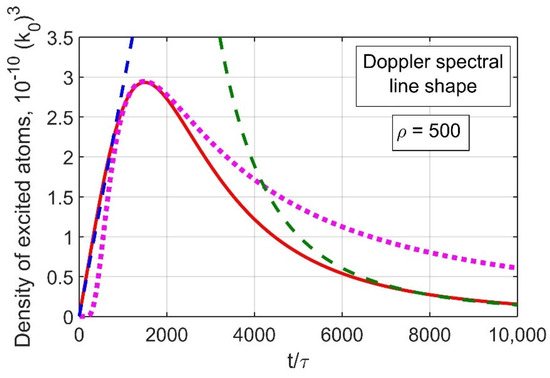
Figure 1.
Comparison of Veklenko’s [12] solution (5) (solid red curve) with asymptotics far in advance of the propagation front (10) (dashed blue curve) and far behind the propagation front (11) (dashed green curve) and with ordinary diffusion Green’s function (dotted magenta curve).
Note that Equation (11) generalizes the results obtained in [30] for the Green’s function of the three-dimensional radiative transfer in a slab with a one-dimensional instant point source in the form of a plane: the asymptotics far behind the propagation front does not depend on spatial coordinates and can be expressed explicitly in terms of the propagation front.
2.1.3. Approximate Self-Similar Solution
It appears that the asymptotic laws of Equations (10) and (11) for the Green’s function for, respectively, far behind and far ahead of the propagation front may be unified in a single interpolation formula. It is worth leaving functional freedom of the interpolation between Equations (10) and (11). This gives:
where G (2) is the kernel of the Biberman–Holstein Equation (1). The mathematical expression of g function in the intermediate region is unknown, but its asymptotic behavior is known:
The procedure of the reconstruction of the function g via comparing the self-similar solution (12) with the exact solution of Equation (1) is as follows:
where G−1 is the function reciprocal to the G function,
where the functions t(ρ,s) and ρ(t,s) are determined by the relation
The accuracy of the proposed self-similar solution strongly depends on the weakness of the dependence (independence) of QG1 and QG2 functions on, respectively, space coordinate and time. The results of the validation of the self-similar solution, including the reconstruction of the function g from the comparison of function (12) with computations of the Green’s function for the Doppler, Lorentz, Voigt, and Holtsmark line shapes, are given in Section 3.3.
The success of the above approach in the case of the Biberman–Holstein radiative transfer in spectral lines of atoms and ions in gases and plasmas has suggested the possibility to extend such an approach to a wider class of nonlocal transport problems. This class is characterized by a model step-length PDF with the arbitrary power-law exponent, which corresponds to the nonlocal (superdiffusion) transport. We start with the one-dimensional (1D) case and infinite velocity of carriers (Section 2.2) and continue with the cases of 1D, 2D, and 3D transport and the finite velocity of carriers (Section 2.3).
2.2. A Method of Deriving an Self-similar Green’s Function for Lévy Flights (Simple Step-Length PDF, C = ∞, 1D Case)
We consider the 1D transport on a uniform background when the retardation caused by the finite velocity of carriers may be neglected. The equation for spatial density f(x, t) of an excitation of the background medium has the form similar to that of the Biberman–Holstein equation: the space-time evolution of the medium’s excitation is governed by the exchange of excitation between various points of the medium via emission and absorption of the carriers:
where W(x) is the probability that the carrier, emitted at some point, is absorbed at a distance x from that point, 1/τ is the absolute value of the emission rate (i.e., τ is the average waiting time between the absorption and reemission of the carrier), q is the source function, which is the rate of production of excitation by an external source (i.e., a source that differs from the excitation of the medium due to absorption described by the W function), and σ is the rate of the quenching of excitation. The uniformity of the background assumes that, first, W is a function of only one variable (the distance between the points of emission and absorption), and second, τ and σ are the constants. Similarly, in the case of the Biberman–Holstein equation, the simplicity of the contribution of quenching to the Green’s function through the function exp(−σt) allows us to set σ = 0. Hereafter, we use the dimensionless time and space coordinate, assuming the normalization of time by τ and using a dimensionless PDF. A search for the Green’s function assumes by definition taking the source function as a point instantaneous source,
Contrary to the case of the Biberman–Holstein equation, we take the kernel of the integral term in the following simple form that possesses a long-tail and the infinite value of the mean square displacement:
The upper bound for parameter γ corresponds to the boundary between the superdiffusive evolution of the Green’s function and the diffusive, Brownian one. It is worth introducing the probability, T(ρ), for the carrier to pass, without any absorption, the distance not exceeding a certain value, ρ. This function is related to the step-length PDF, , of Equation (21) (the relation between and is shown for the 1D case):
The power-law dependence assumed in Equation (21) takes please, e.g., in two well-known cases of the transport by resonant photons, namely, Lorentz and Doppler spectral line shapes (cf. (A6) and (A7) in the Appendix in [41] and (38) in [16]), where the exponent γ essentially depends on the tail of the line shape. Note also that there is an example of a physics model which gives the power-law step-length PDF (22): see Equation (1) in [32] for photon-assisted transport of minority carriers in semiconductors (photo-excited holes in n-type InP [33]).
The Green’s function of Equation (19) shows asymptotic behavior similar to that in the case of the Biberman–Holstein equation. Far in advance of the propagation front arrival at a distance ρ, ρ ρfr(t) 1, where the propagation front is defined by Equation (7) (or, equivalently, for a short time, 1 t tfr(ρ)), the density is determined by the direct population by the carriers emitted by the source. This gives a simple relation (cf. (10))
The asymptotics of the Green’s function far behind the propagation front, ρ ρfr(t), or equivalently t tfr(ρ)) 1, may be found taking into account the above-mentioned frequent exchange with short-free-path carriers. The latter produces local uniformity of the density. Assuming a plateau-like spatial distribution around the origin, one has (cf. (11)):
The approximate self-similar solution is suggested in the form of Equation (12) which takes the form
where g is an unknown function of a single variable with the asymptotics (13), (14).
A test of solutions for the Green’s function (25), its asymptotics (13) and (14), and propagation front (7), via comparison with the direct numerical solution of Equation (19) may be considered as an inverse problem of reconstructing the function g or, equivalently, as a proof of the scaling law (self-similarity of solutions) formulated with Equations (25), (13), (14), and (7). The results of reconstructing the function g presented in Section 3 show how the function g behaves at s ~ 1 and smoothly goes to values proportional to s at s ≫ 1.
We try the validity of the method in the case of a simple PDF with a power-law tail. We consider the following case:
The analytic solution of (19) with the PDF (26) has the form [41]:
The approximate self-similar solution of Equation (19) with the kernel (26) may be obtained from Equation (25):
where asymptotic of the function g obeys Equations (13), (14), and
In the case of PDF (26), Equation (14) may be specified:
where Γ is the Euler gamma function. The procedure of the reconstruction of the function g via comparing the self-similar solution (28) with the exact solution (27) is quite similar to that of Equations (15)–(17) and can be described by the following equation:
where the functions t(ρ,s) and ρ(t,s) are determined by the relation
Note that the propagation front (29) is a partial case of the relation defined by (34): ρfr(t) = ρ(t, s = 1).
2.3. A Method of Deriving a Self-Similar Green’s Function for Lévy Walks (Simple Step-Length PDF, , 1D, 2D and 3D Cases)
2.3.1. General Solution of the Time-Dependent Superdiffusive Transport Equation
We consider superdiffusive transport processes that are either transfer of an excitation of an immobile homogeneous medium by carriers not belonging to the medium (e.g., processes described by the equation for the density of excited atoms or ions in the plasma at the transfer of the atomic excitation by resonant photons) or the dynamics of objects or subjects that move (migrate) on a homogeneous plane or volume at the same velocity between stop points at a given average residence time (waiting time) at stop points. Then, the equation for the Green’s function of the excitation of the medium or the density of migrants at rest at the point and time t has the form (this equation is an analog of Equation (1) in [48]):
Here, is the constant velocity of carriers between stop points, and has the same meaning as in (1), is the Heaviside step function, is the Dirac delta function, and is the probability of absorption of the carrier (or the probability of stop of the carrier) at the distance from the point of its last start, normalized as
Here, is a volume element in the space (): in the one-dimensional case , in the two-dimensional case and in the three-dimensional case . Moreover, the function
is a step-length (i.e., free path) PDF for the carriers of the medium’s perturbation or of the running migrants. In the case of PDF with a power-law tail (26), we can obtain the general solution in 1D [48], 2D, and 3D cases [49]:
Here,
is the ratio of the average lifetime of the excited state to the mean free time of flight of a carrier (photon) or the ratio of the average times in the rest and motion states of a migrant, is the zeroth-order Bessel function.
2.3.2. Asymptotics of the Green’s Function Far Ahead and Far behind the Perturbation Front
The asymptotics far ahead of the propagation front can be obtained from the general solution for the Green’s function, taking the limit , since the coordinate values are bounded from above by the ballistic front . In the one-dimensional case, the direct calculation gives the following result [46] (here, the length and time are measured in units of and , respectively):
It was shown [49] that this expression is also valid for two-dimensional and three-dimensional cases. Note that as , which corresponds to the transition from Lévy walks to Lévy flights, (42) coincides with (23).
The asymptotics far behind the propagation front correspond to taking the limit . In contrast to Lévy flights for Lévy walks, in the general case, it is not possible to obtain an expression for this asymptotics; however, in the particular case , which corresponds to the case of the Lorentz shape of the wings of the photon emission spectral line, an approximate expression can be obtained. In the 1D case, large values of retardation parameter and even larger values of time, the calculation of (38) gives the result [48], which coincides with the scaling law (19) in [6] and determines the numerical coefficient in this scaling:
2.3.3. Integral Characteristics of Green’s Function
The number of excited particles in a medium for the problem of radiative transfer in a homogeneous medium (or migrants at rest for the problem of migration in a homogeneous medium) at time can be obtained by integrating the Green’s function (38)–(40) over the space:
It appears that this function does not depend on the dimensionality of the coordinate space. The expression for at may be obtained analytically [49]:
Note that (this follows from the definition of the source in the Equation (35) for the Green’s function); therefore, is the fraction of excited particles in the total number of particles in the medium or the fraction of migrants at rest in the total number of migrants. The result (45) means that the number of excited particles (or migrants at rest) can tend to either zero or nonzero constant, highly depending on of the model step-length PDF (37), (26). For , Equation (45) coincides within a constant with the scaling law obtained in [6] (see (18) therein for ).
2.3.4. Approximate Self-Similar Solution and Test of Its Accuracy
Following the method proposed in [41] and generalized in [48] to the case of a finite velocity of carriers, we construct an approximate self-similar solution in the form [48,49]:
Here, is the self-similarity function with the asymptotic limits
and is the propagation front defined similarly to Equation (8) in [48] and Equation (4.3) in [49], i.e., from the equality of the asymptotic expression for the exact solution near the ballistic cone (in dimensionless variables) to the exact solution at the point of the source of the perturbation (coordinate’s origin):
The validity of self-similar solution given by Equation (46) in a broad range of space-time and other variables of the problem is proved both for the one-dimensional case [48] and for the two- and three-dimensional cases [49].
Following the method suggested in [41,48,49] to estimate the accuracy of the proposed self-similar solution, we introduce the self-similarity function through the relation
To test the accuracy of the indicated self-similarity, it is necessary to show that the function weakly depends (or does not depend) on time:
2.4. Distributed Computing Parameters and Implementation for Verification for Accuracy of the Approximate Self-Similar Solution
Obtaining self-similar solutions in the entire space of independent variables requires mass numerical simulations; however, their total volume is significantly reduced due to self-similarity of the solution.
We carried out massive computations of the exact solution of the transport equation and compared these results with self-similar solutions to verify their accuracy and to identify the limits of their applicability.
Computations have been performed on the cluster HPC4, http://computing.nrcki.ru/ (accessed on 26 February 2021), at the NRC Kurchatov Institute. Operational access to the cluster has been provided by a special agent of Everest, http://everest.distcomp.org/ (accessed on 26 February 2021), a computing platform to integrate applications running on distributed heterogeneous computing resources [58]. General-purpose Everest application, Parameter Sweep [59], http://everest.distcomp.org/docs/ps (accessed on 26 February 2021), was used to run independent Everest tasks on the cluster’s working nodes.
2.4.1. A Test of the Proposed Self-Similar Solution for a Simple Model PDF, 1D Case
In order to obtain the self-similarity functions g(s) for different values of γ, the exact solutions fexact(ρ,t) were calculated. The values of t were evenly spaced on a log scale (100 points per power) in the range from tmin = 30 to tmax = 108, creating the numerical mesh of a total of 653 points. The values of s were also evenly spaced on a log scale (50 points per power) in the range from smin = 0.01 to smax = 1000, creating the numerical mesh of a total of 501 points. The respective values of ρ are defined by these two numerical meshes using (34). The values of γ were evenly spaced in the range from γmin = 0.5 to γmax = 1.5, creating the numerical mesh of a total of 101 points. We used distributed computing to calculate fexact(ρ,t) on these meshes.
We had to solve 101 independent tasks that correspond to the mesh of variable γ. All analytic Expressions (27)–(34) have been implemented in the form of a Python program, using NumPy and SciPy, well-known scientific libraries (www.scipy.org, (accessed on 26 February 2021)).
The less value of γ, the more time is spent for computation, e.g., for γ = 0.5, computations took 8.5 h on a single core of Intel Xeon E5-2650v2 CPU. Some tests have been performed via the Parameter Sweep, a special Everest application mentioned above. It was found that the available implementation of the Everest-agent for the SLURM (see agent’s sources at https://gitlab.com/everest/agent, (accessed on 26 February 2021)) has a limit on the number of tasks running in parallel on the cluster (not more than 64). The final computations have been carried out by the SLURM commands directly from the master host.
2.4.2. A Test of the Self-Similar Solution of Biberman–Holstein Equation
The calculation of exact and self-similar solutions for a single value of parameter a in the Voigt spectral line shape (53) was an independent task, such as the case of the Doppler or Lorentz line shape. The values of a were taken in the range from 0.01 to 10, evenly spaced on a log scale, that yields 28 tasks. We analyzed the self-similar solutions for two different expressions for the propagation front, Equations (7) and (8); therefore, the total number of independent tasks was 56.
The self-similarity function g(s) was reconstructed using the calculated exact solutions fexact(ρ,t). The values of t were evenly spaced on a log scale in the range from tmin = 30 to tmax = 108. The values of s were also evenly spaced on a log scale. For the Voigt line shape, depending on the value of a, the lower limit for s was set in the range from 0.00003 (small a) to 0.005 (large a), whereas the upper limit was set to 1000 for all values of a. The respective values of ρ are defined by the t and s numerical meshes, using (18).
All analytic Expressions (12)–(18) have been implemented in the form of a Python program, using NumPy and SciPy, well-known scientific libraries (www.scipy.org).
Besides direct comparison of the self-similar (12) and exact (5) solutions of the transport Equation (1), the range of variables in the two-dimensional space, {time, space coordinate}, where the self-similar solution is accurate within certain error bars around the exact solution, was identified.
3. Results
3.1. Illustration of Nonlocality by Monte Carlo Calculations of Trajectories
Figure 2 shows typical examples of a trajectory of the Lévy flight type: starting from the zero point in time, a migrant stands time t, which is a random variable determined by the waiting time PDF
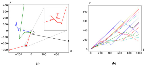
Figure 2.
Typical trajectories of migrants, standing at the origin at the zero point in time, for a period of time 1000, , (a) Four trajectories in the dimensionless coordinates (i.e., multiplied by ). The stops are shown as dots. Long runs (Lévy flights) connect sections with short (Brownian-like) walks (see inset in the figure). (b) Twelve trajectories in coordinates .
(time is dimensionless), then begins to move with equal probability in any direction (i.e., uniformly in angle in the plane of motion) along a straight path with a constant velocity and travels the random distance determined by the step-length PDF (37), then stops again, and so on.
One can see the characteristic feature of trajectories with long steps (Lévy flights), which connect the clusters of (mostly multiple) short steps which form a walk of the Brownian type. Artificial (synthetic) experimental data for , , were prepared using the pseudo-random number generator.
3.2. A Test of the Proposed Self-Similar Solution (Simple Step-Length PDF, , 1D Case)
Besides direct comparison of the self-similar, (28), and exact, (27), solutions of the transport Equation (19), an inverse problem is solved to identify the range of variables in the two-dimensional space, {time, space coordinate}, where the self-similar solution is accurate within 10% error bars around the exact solution. This boundary, dubbed t10%, as a function of time only, i.e., for the entire range of space coordinates, is shown in Figure 3.
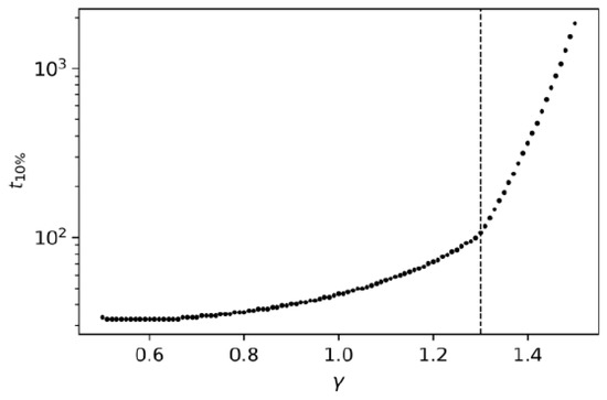
Figure 3.
The values of time, t10%, for which the condition 0.9 ≤ fauto(ρ,t > tmin)/fexact(ρ,t > tmin) ≤ 1.1 is met for various values of γ.
The minimal value, γ = 0.5, corresponds to the longest tail of the PDF of the type (26), known in physical problems (see, e.g., [16]). The maximal value, γ = 1.5, corresponds to the case, which is close enough to the boundary between the superdiffusive and diffusive evolution.
Analysis of self-similar solutions is illustrated with Figure 4, Figure 5 and Figure 6 for three values of γ. Each case is represented with three figures. The functions Qw(s,t) (33) are shown for different values of t in the range from t10%(γ) to tmax = 108. The normalized functions Qw(s,t)/{Qw}av(s), where subscript av denotes averaging over time from tmin = 30 to tmax = 108, and the relative errors of the self-similar solution fauto(ρ,t)/fexact(ρ,t) are shown for the same range of time.
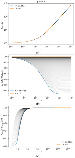
Figure 4.
Functions QW(s,t) (33) for γ = 0.5 and different values of t in the range from t10% = 33.66 to tmax = 108 (a). Normalized functions QW(s,t)/{QW}av(s) for the same range of t (b). The relative errors of the self-similar solution, fauto(ρ,t)/fexact(ρ,t), for the same range of t (c).
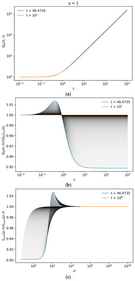
Figure 5.
The same plots as in Figure 4 but for γ = 1.0 and the values of t in the range from t10% = 46.47 to tmax = 108 (a). Normalized functions QW(s,t)/{QW}av(s) for the same range of t (b). The relative errors of the self-similar solution, fauto(ρ,t)/fexact(ρ,t), for the same range of t (c).
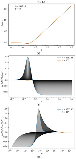
Figure 6.
The same plots as in Figure 4 but for γ = 1.5 and the values of t in the range from t10% = 1853.15 to tmax = 108 (a). Normalized functions QW(s,t)/{QW}av(s) for the same range of t (b). The relative errors of the self-similar solution, fauto(ρ,t)/fexact(ρ,t), for the same range of t (c).
The results shown in Figure 4, Figure 5 and Figure 6 illustrate the following main features of the superdiffusivity as itself and of the self-similar solutions. If the region in {t, ρ} space, where 10% error is not exceeded, is identified (Figure 4c, Figure 5c and Figure 6c), the region, where maximal error is located, moves from the point {tmin, 0} for γ < 1.3 to the region s~0.2 for γ > 1.3 (Figure 4b, Figure 5b and Figure 6b). This corresponds to a kink in the curve in Figure 3, marked with a vertical line. The self-similar function g(s), as a function of a single variable, is formed with high accuracy in the very wide range of {t, ρ} space (Figure 4a, Figure 5a and Figure 6a). The highest superdiffusivity, being produced by the longest tail of the PDF, needs, as expected, the longest computation time of the exact solution, whereas the applicability of the self-similar solutions is limited only by the expected violation at not large values of time. This illustrates the importance of self-similar solutions for the most time-consuming problems.
3.3. Verification for Accuracy of the Approximate Self-Similar Solution for Various Spectral Line Shapes (Biberman–Holstein Step-Length PDF, , 3D Case)
3.3.1. Lorentz Spectral Line Shape
The line shape εν and respective absorption coefficient kν are taken in the form [12]:
Here, is the full width at half maximum (FWHM) of the Lorentz line shape.
To prove the self-similar solution, one has to show weak dependence (independence) of QG1 and QG2 functions on, respectively, space coordinate and time. The results of the validation of the self-similar solution and the reconstruction of function g from comparison with exact solution (5), using (51) for εν and kν, with the help of Equations (15) and (16) are shown in Figure 7a,b.
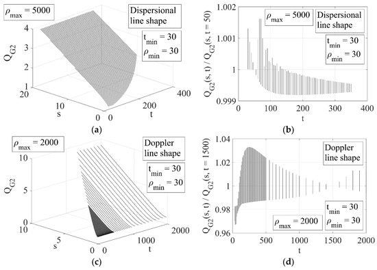
Figure 7.
The self-similar function g in Equation (12), reconstructed from comparison with the exact solution with the help of Equations (15) and (17) for Lorentz and Doppler spectral line shapes. Function QG2 for ρ > ρmin, t > tmin for (a) dispersional (Lorentz) and (c) Doppler spectral line shapes. Projection of the ratio QG2(s, t)/QG2(s, t*) onto the {QG2, t} plane for (b) dispersional (Lorentz), t* = 50, and (d) Doppler, t* = 1500, spectral line shapes. The dependence of the error, which is given by the deviation from unity, on the tmin value is shown in the right-hand-side figures. The range of variable s is limited by the conditions ρ < ρmax.
3.3.2. Doppler Spectral Line Shape
The line shape εν and respective absorption coefficient kν are taken in the form [12]:
Here, is the full width at half maximum (FWHM) of the Doppler line shape.
The results of the validation of the self-similar solution and the reconstruction of function g from comparison with exact solution (5), using (52) for εν and kν, with the help of Equations (15) and (17) are shown in Figure 7c,d.
3.3.3. Voigt Spectral Line Shape
The line shape εν is taken in the form [51]:
where:
Here, is the full width at half maximum (FWHM) of the Doppler line shape, and is the FWHM of the Lorentz line shape. The coefficient is determined by the normalization condition, . For the Stark broadening of the spectral line shape, one may use the well-known formulae for the impact broadening, e.g., in the monographs and reviews [52,53,54,55,56,57].
The respective absorption coefficient kν(a) has the form
where n0 is the density of absorbing atoms, λ is the wavelength of a photon, and is the statistical weight of the i-th level.
The exact solution in this case has the form
The accuracy analysis is illustrated with three figures. The absolute values of the self-similarity functions QG2(s,t) (17) are shown for different values of t in the range from tmin = 30 to tmax = 106. The normalized values of these functions are defined as QG2(s,t)/{QG2}av(s), where subscript av denotes averaging over time from tmin = 30 to tmax = 108. These normalized functions and the relative errors of the self-similar solution fauto(ρ,t)/fexact(ρ,t) are shown for the same range of time.
The results of accuracy analysis for various values of the Voigt parameter a are shown in Figure 8 (see [45] for more detailed results).
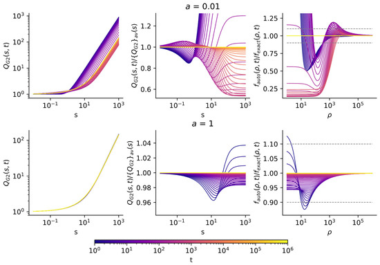
Figure 8.
The result of accuracy analysis of self-similar solution for various values of the Voigt parameter and the propagation front ρ = ρfr taken in the form of Equation (7), for different values of t in the range from tmin = 30 to tmax = 106: (left) functions QG2(s,t) (17); (center) normalized functions QG2(s,t)/{QG2}av(s), where subscript av denotes averaging over time from tmin = 30 to tmax = 108; (right) relative errors of the self-similar solution fauto(ρ,t)/fexact(ρ,t).
The limits of applicability of the self-similar solutions with a certain accuracy are illustrated with Figure 9, where the level lines of the relative deviation of the self-similar solution from the exact one, for the results from Figure 8, are shown. It is seen that for moderate and large values of the Voigt parameter a when the Lorentz line shape dominates in the Voigt line shape, the accuracy of the self-similar solution is high in almost the entire space of variables {ρ, t}, quite similar to the case [41,47] of the superdiffusive transport for a 1D model PDF with the power-law wings. However, for a small a, the accuracy of self-similar solution dramatically falls down in the essential part of the space of variables {ρ, t}. It was this failure that stimulated our quest to improve the accuracy and offer the propagation front in the form of Equation (8). The results for the propagation front (8) are shown in Figure 10 and Figure 11.
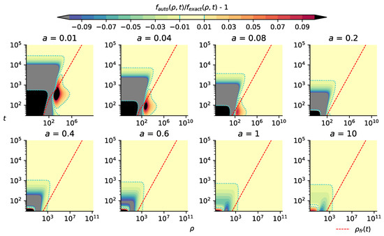
Figure 9.
The level lines of the relative deviation of the self-similar solution from the exact one, for the results from Figure 8. The propagation front (7) is shown with a red dashed line.
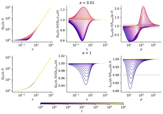
Figure 10.
The same as in Figure 8 but for the propagation front ρ = ρfr taken in the form (8).
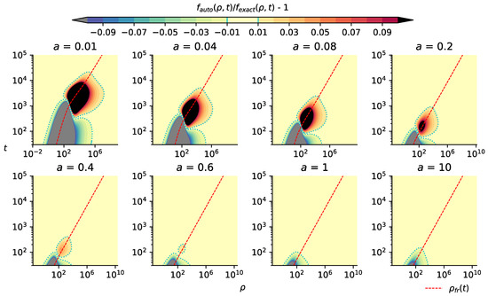
Figure 11.
The same as in Figure 9 but for the propagation front ρ = ρfr (red dashed line) taken in the form (8).
Note that the sudden transition from large positive to large negative values (i.e., from black to gray) in the figures in the top row of Figure 9 corresponds to similar behavior of the relative error of the approximate self-similar Green’s function with respect to the exact calculation of the Green’s function for a = 0.01 in Figure 8, top row, right side.
Figure 9 and Figure 11 show that the self-similar solution with the propagation front (8) substantially improves the accuracy in the regions of the failure of the self-similar solution with the propagation front (7). This issue points to the possibility to further improve the accuracy by the variation of the definition of the propagation front and further verification of the accuracy of the respective self-similar function via calculations of the exact solution in a limited part of the space of variables {ρ, t} (not in the entire space, only in the region around the propagation front).
3.3.4. Holtsmark Spectral Line Shape
For Holtsmark spectral line shape, the functions εν and kν, which enter the function J(p), for linear Stark effect may be expressed in the form (cf. [54]):
where N is the density of the perturbing particles, , the Holtsmark function:
The exact solution (5) with using (60) and (61) for εν and kν, , takes the form:
Figure 12 (see [45] for more detailed results) shows the behavior of the self-similar function QG2 (17) and the relative deviation of the self-similar solution from the exact one in the range from tmin = 40 to tmax = 103, with the time step equal to 20, for 40 ≤ t ≤ 500, and 50, for 500 < t ≤ 1000.
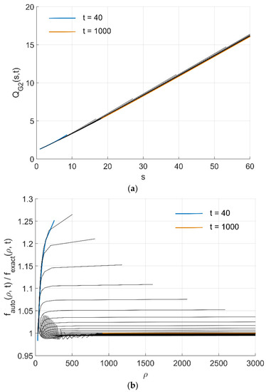
Figure 12.
The result of accuracy analysis of self-similar solution for the propagation front ρ = ρfr taken in the form (7), for different values of t in the range from tmin = 40 to tmax = 103 with the time step equal to 20, if 40 ≤ t ≤ 500, and 50, if 500 < t ≤ 1000: (a) functions QG2(s,t) (17); (b) relative error of the self-similar solution, fauto(ρ,t)/fexact(ρ,t).
The results show that, similarly to the 1D transport for a model step-length PDF with power-law wings [41,47], the accuracy of self-similar solution for the 3D radiative transfer for the Holsmark spectral line shape is reasonably good for the propagation front (7).
3.4. Verification for Accuracy of the Approximate Self-Similar Solution for Lévy Walks (Simple Step-Length PDF, , 1D, 2D and 3D Cases)
The self-similar solution (46) and the propagation front (48) are determined by the asymptotics of the Green’s function; therefore, it is important to understand in which region of the variables the asymptotics work well. Figure 13 and Figure 14 show the solution of Equation (35) by the Monte Carlo method for a two-dimensional transport (blue curve), the asymptotics (42) of the Green’s function near the ballistic cone (orange dashed curve), the propagation front (48) (vertical black dotted line), for , , (Figure 13), and (Figure 14). It can be seen that with increasing , the region in which the asymptotic expression is well applicable increases.
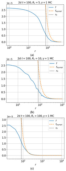
Figure 13.
The solution for the Green’s function (35) by the Monte Carlo method for two-dimensional transport (blue curve); the asymptotics of the Green’s function near the ballistic cone (42) (orange dashed curve); the front law (48) (vertical black dotted line) for (a) (b) (c) , and .
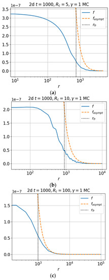
Figure 14.
Same as in Figure 13, but for .
The accuracy of the asymptotics of the Green’s function near the ballistic cone in the 1D case for and was shown in Figures 1–6 in [48].
The dependence of the self-similarity function (50) for and on at various times in the interval for (a,b) three- and (c–g) two-dimensional cases is shown in Figure 15. In the 3D case, a direct numerical calculation of the Green’s function (40) was used. In the 2D case, simulation of trajectories produced by the Monte Carlo method was applied. Figure 15 demonstrates the accuracy of self-similar solution (46). It is seen that the curves in Figure 15 are in agreement. In particular, a linear growth of the self-similarity function is well observed in the region of the self-similar variable.
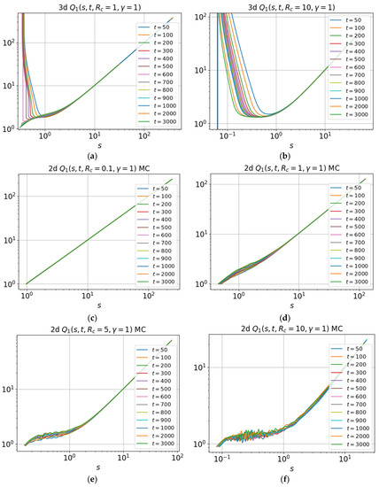
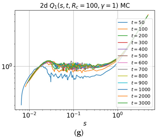
Figure 15.
Self-similarity function (50) for and versus at different times in the (a,b) three- and (c–g) two-dimensional cases.
We also analyze the relative deviation of the function from the function for , and , shown in Figure 15 for the (a,b) three- and (c–g) two-dimensional cases. We consider the deviation of approximate self-similar solution from the exact solution, using for the self-similar solution the self-similarity function taken at the maximum considered time . This is because the time dependence of the self-similarity function is weakened with increasing . The maximum relative deviation of the self-similarity function for relatively small is ~100% for the three-dimensional case and is ~85% for the two-dimensional case. As seen in Figure 15, the maximum deviation corresponds to the region of small values. It should also be noted that with increasing time, self-similarity increases, as can be seen from Figure 15 and Figure 16.
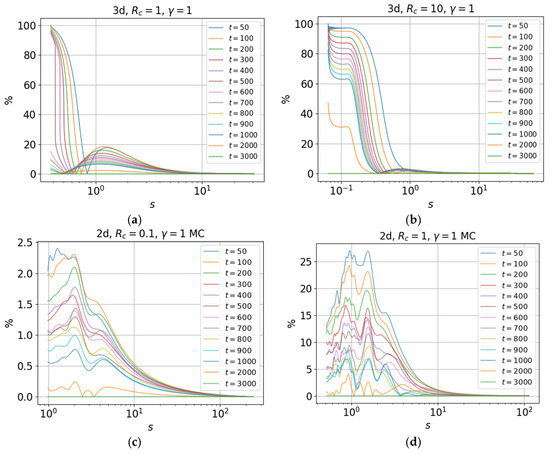
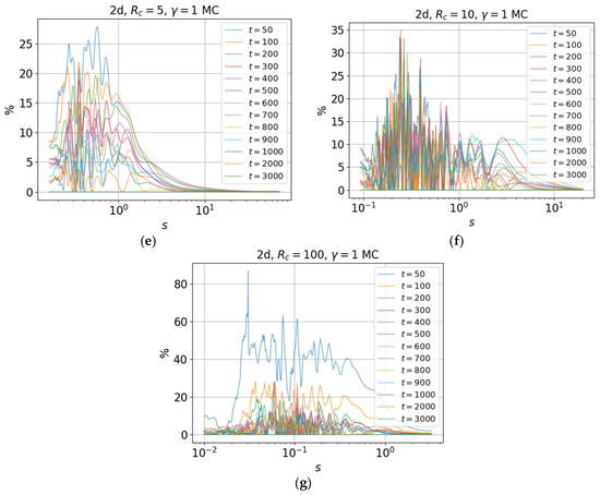
Figure 16.
Relative deviation of the self-similarity function (50) for and versus at different times in the (a,b) three- and (c–g) two-dimensional cases.
As increases, the function becomes linear and deviation tends to zero. Approximate self-similar solutions (46) obtained using the existing self-similarity functions with the wide range of parameters and are plotted by dotted lines in Figure 17 for (a,b) three- and (c–g) two-dimensional cases for various times together with the numerically calculated general solutions given by Equation (40) (in 3D case) and simulation of trajectories of (35) produced by the Monte Carlo method shown by solid lines (in 2D case).
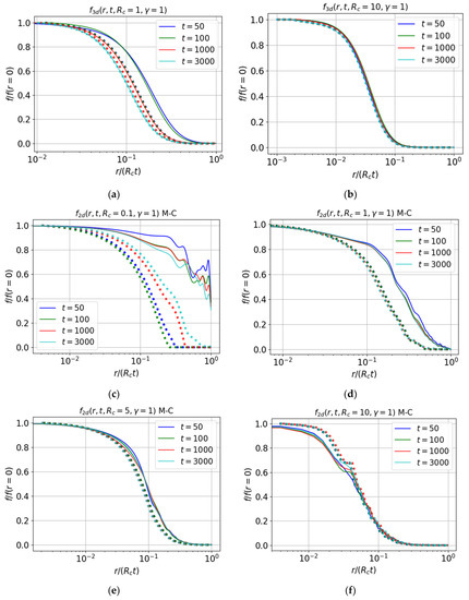
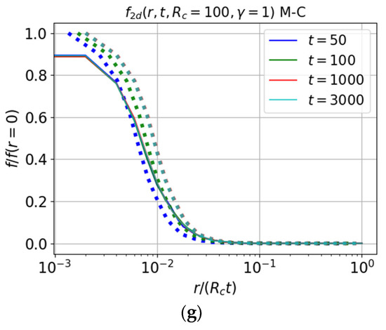
Figure 17.
Self-similar solutions (46) constructed from the self-similarity function at the maximum time (dotted lines); general solutions (40) (solid lines). (a,b) Direct calculation of the Green’s function (40) in the three-dimensional case; (c–g) Monte Carlo simulation of trajectories in accordance with the transport Equation (35) in the two-dimensional case. Results are presented for and .
The self-similarity function (50) in the 1D case for and was shown in Figures 7 and 9 in [48]; in the 2D and 3D cases, for and , in Figure 4 in [49]. The relative deviation of the self-similarity function (50) in the 1D case, for and was shown in Figures 8 and 10 in [48]; in the 2D and 3D cases, for and , in Figure 5 in [49].
Figure 17 shows the results for the normalized Green’s function as a function of the normalized coordinate for . For the three-dimensional case, the maximum relative deviation of the approximate self-similar solution from the exact one is about 40% for parameter (Figure 17a), in the case of the deviation is about 1% (Figure 17b). In the two-dimensional case, we see an increase in the accuracy of the approximate self-similar solution with increasing (however, for , the Monte Carlo calculations are less accurate, and the respective propagation front and self-similar solution are also less accurate).
The accuracy of the self-similarity solution (46) in the 1D case for and was shown in Figures 11 and 12 in [48]; in the 2D and 3D cases, for and , in Figures 6 and 7 in [49].
4. Discussion
Here is an overview of the results of the work [41,42,43,44,45,46,47,48,49,50] aimed at creating a new method in the theory of nonstationary nonlocal transport (superdiffusion, going beyond the standard Brownian diffusion). It is appropriate to call this method the interpolated self-similarity method. The method is based on an algorithm for obtaining an approximate self-similar solution for the Green’s function of a wide class of integro-differential equations of nonstationary transport, covering transport phenomena with a dominant contribution of carriers with a large free path: Lévy flights [1,2,3,4], including the problem of nonstationary transport of resonance radiation in the Biberman–Holstein model [9,10,11,12,13,14,15,16,17,18,19,20,29,30], or, in the case of taking into account the finite velocity of carriers, Lévy walks [5,6,7], or more precisely, Lévy walk with rests (see Figure 1 in the review [7]), which covers such problems as the transfer of resonance radiation in astrophysical gases and plasma, biological migration, and energy transfer by waves in plasmas. The method is based on the interpolation of self-similarity laws for asymptotics far ahead and far behind the effective front of the medium’s perturbation propagation, which requires a direct solution of the problem (numerical calculation of the Green’s function) only in a relatively small range of problem variables. We believe that it is of great interest for the significant reduction of numerical calculations in numerous applied problems of superdiffusive transport in physics and other sciences.
Author Contributions
Conceptualization, A.B.K.; methodology, all co-authors; software, A.A.K., V.S.N., and A.V.S.; validation, A.A.K. and P.A.S.; formal analysis, A.A.K. and P.A.S.; resources, V.V.V.; data curation, V.S.N. and V.V.V.; writing—original draft preparation, P.A.S. and A.A.K.; writing—review and editing, A.B.K.; visualization, V.S.N., A.A.K., P.A.S., and A.V.S. All authors have read and agreed to the published version of the manuscript.
Funding
This work was supported in part by the Russian Foundation for Basic Research: project nos. 18-07-01269-a, 19-32-90281, and 20-07-00701-a.
Institutional Review Board Statement
Not applicable.
Informed Consent Statement
Not applicable.
Data Availability Statement
Not applicable.
Acknowledgments
This work has been carried out using computing resources of the federal collective usage center Complex for Simulation and Data Processing for Megascience Facilities at NRC Kurchatov Institute, http://ckp.nrcki.ru/.
Conflicts of Interest
The authors declare no conflict of interest.
References
- Shlesinger, M.; Zaslavsky, G.M.; Frisch, U. (Eds.) Lévy Flights and Related Topics in Physics; Springer: Berlin, Germany, 1995; ISBN 978-3-662-14048-2. [Google Scholar]
- Dubkov, A.A.; Spagnolo, B.; Uchaikin, V.V. Lévy flight superdiffusion: An introduction. Int. J. Bifurc. Chaos 2008, 18, 2649–2672. [Google Scholar] [CrossRef]
- Klafter, J.; Sokolov, I.M. Anomalous diffusion spreads its wings. Phys. World 2005, 18, 29–32. [Google Scholar] [CrossRef]
- Eliazar, I.I.; Shlesinger, M.F. Fractional motions. Phys. Rep. 2013, 527, 101–129. [Google Scholar] [CrossRef]
- Shlesinger, M.F.; Klafter, J.; Wong, Y.M. Random walks with infinite spatial and temporal moments. J. Stat. Phys. 1982, 27, 499–512. [Google Scholar] [CrossRef]
- Zaburdaev, V.Y.; Chukbar, K.V. Enhanced superdiffusion and finite velocity of Lévy flights. J. Exp. Theor. Phys. 2002, 94, 252–259. [Google Scholar] [CrossRef]
- Zaburdaev, V.; Denisov, S.; Klafter, J. Lévy walks. Rev. Mod. Phys. 2015, 87, 483. [Google Scholar] [CrossRef]
- Mandelbrot, B.B. The Fractal Geometry of Nature; W. H. Freeman: New York, NY, USA, 1982; ISBN 0-7167-1186-1189. [Google Scholar]
- Biberman, L.M. On the diffusion theory of resonance radiation. Zh. Eksp. Teor. Fiz. 1947, 17, 416. [Google Scholar]
- Holstein, T. Imprisonment of Resonance Radiation in Gases. Phys. Rev. 1947, 72, 1212–1233. [Google Scholar] [CrossRef]
- Biberman, L.M.; Vorob’ev, V.S.; Yakubov, I.T. Kinetics of Nonequilibrium Low Temperature Plasmas; Consultants Bureau: New York, NY, USA, 1987; ISBN 978-1-4684-1667-1. [Google Scholar]
- Veklenko, B.A. Green’s Function for the Resonance Radiation Diffusion Equation. Sov. Phys. JETP 1959, 36, 138–142. [Google Scholar]
- Biberman, L.M. Approximate method of describing the diffusion of resonance radiation. Dokl. Akad. Nauk. SSSR Ser. Phys. 1948, 59, 659. (In Russian) [Google Scholar]
- Kogan, V.I. A Survey of Phenomena in Ionized Gases (Invited Papers). In Proceedings of the ICPIG’67, Vienna, Austria, 27 August–2 September 1968; p. 583. (In Russian). [Google Scholar]
- Kogan, V.I. Encyclopedia of Low Temperature Plasma. Introduction Volume; Fortov, V.E., Ed.; Nauka/Interperiodika: Moscow, Russia, 2000; Volume 1, p. 481. (In Russian) [Google Scholar]
- Abramov, V.A.; Kogan, V.I.; Lisitsa, V.S. Radiative transfer in plasmas. In Reviews of Plasma Physics; Leontovich, M.A., Kadomtsev, B.B., Eds.; Consultants Bureau: New York, NY, USA, 1987; Volume 12, p. 151. [Google Scholar]
- Kalkofen, W. (Ed.) Methods in Radiative Transfer; Cambridge University Press: Cambridge, UK, 1984; ISBN 0-521-25620-8. [Google Scholar]
- Rybicki, G.B. Escape Probability Methods. In Methods in Radiative Transfer; Kalkofen, W., Ed.; Cambridge University Press: Cambridge, UK, 1984; Chapter 1; ISBN 0-521-25620-8. [Google Scholar]
- Napartovich, A.P. On the τeff method in the radiative transfer theory. High. Temp. 1971, 9, 23–26. [Google Scholar]
- Biberman, L.M.; Vorob’ev, V.S.; Lagar’kov, A.N. Radiative transfer in ionization continuum. Opt. Spectrosc. 1965, 19, 326. (In Russian) [Google Scholar]
- Kukushkin, A.B.; Lisitsa, V.S.; Savel’ev, Y.A. Nonlocal transport of thermal perturbations in a plasma. JETP Lett. 1987, 46, 448–451. Available online: http://www.jetpletters.ac.ru/ps/1232/article_18610.pdf (accessed on 26 February 2021).
- Rosenbluth, M.N.; Liu, C.S. Cross-field energy transport by plasma waves. Phys. Fluids 1976, 19, 815–818. [Google Scholar] [CrossRef]
- Kukushkin, A.B. Analytic description of energy loss by a bounded inhomogeneous hot plasma due to the emission of electromagnetic waves. JETP Lett. 1992, 56, 487–491. Available online: http://www.jetpletters.ac.ru/ps/1293/article_19528.pdf (accessed on 26 February 2021).
- Kukushkin, A.B. Heat transport by cyclotron waves in plasmas with strong magnetic field and highly reflecting walls. In Proceedings of the 14th IAEA Conference on Plasma Physics and Controlled Nuclear Fusion Research, Wuerzburg, Germany, 30 September–7 October 1992; International Atomic Energy Agency: Vienna, Austria, 1993; Volume 2, p. 35. [Google Scholar]
- Kukushkin, A.B. Generalized Escape-Probability Method in the Theory of High-Intensity Radiative Transfer in Continuous Spectra. In Proceedings of the AIP Conference Proceedings 299, Dense Z-pinches 3rd International Conference, London, UK, 19–23 April 1993; Haines, M., Knight, A., Eds.; AIP Press: New York, NY, USA, 1994; p. 519. [Google Scholar] [CrossRef]
- Tamor, S. Calculation of Energy Transport by Cyclotron Radiation in Fusion Plasmas. Fusion. Technol. 1983, 3, 293–303. [Google Scholar] [CrossRef]
- Tamor, S. Synchrotron radiation loss from hot plasma. Nucl. Instr. Meth. Phys. Res. 1988, A271, 37–40. [Google Scholar] [CrossRef]
- Tamor, S. A Simple Fast Routine for Computation of Energy Transport by Synchrotron Radiation in Tokamaks and Similar Geometries; Science Applications, Inc.: La Jolla, CA, USA, 1981; Lab. for Applied Plasma Studies Report SAI-023-81-189 LJ0LAPS-72, Science Applications. [Google Scholar]
- Abramov, Y.Y.; Napartovich, A.P. Transfer of resonance line radiation from a point source in the half-space. Astrofizika 1969, 5, 187–202. (In Russian) [Google Scholar]
- Abramov, Y.Y.; Napartovich, A.P. The excitation wave caused by a light flare. Astrofizika 1968, 4, 195–206. (In Russian) [Google Scholar]
- Levinson, I.B. Resonant-radiation transfer and nonequilibrium phonons in ruby. Zh. Eksp. Teor. Fiz. 1978, 75, 234–248. [Google Scholar]
- Subashiev, A.V.; Semyonov, O.; Chen, Z.; Luryi, S. Temperature controlled Lévy flights of minority carriers in photoexcited bulk n-InP. Phys. Lett. A 2014, 378, 266–269. [Google Scholar] [CrossRef]
- Luryi, S.; Semyonov, O.; Subashiev, A.V.; Chen, Z. Direct observation of Lévy flights of holes in bulk n-doped InP. Phys. Rev. B 2012, 86, 201201(R). [Google Scholar] [CrossRef]
- Ivanov, V. Transfer of Radiation in Spectral Lines; NBS Special Publication no 385; US Govt Printing Office: Washington, DC, USA, 1973.
- Mihalas, D. Stellar Atmospheres; Freeman: San Francisco, CA, USA, 1970; p. 399. [Google Scholar]
- Barthelemy, P.; Bertolotti, J.; Wiersma, D.S. A Lévy flight for light. Nature 2008, 453, 495–498. [Google Scholar] [CrossRef] [PubMed]
- Mercadier, N.; Chevrollier, M.; Guerin, W.; Kaiser, R. Microscopic characterization of Lévy flights of light in atomic vapors. Phys. Rev. A 2013, 87, 063837. [Google Scholar] [CrossRef]
- Pereira, E.; Martinho, J.; Berberan-Santos, M. Photon Trajectories in Incoherent Atomic Radiation Trapping as Lévy Flights. Phys. Rev. Lett. 2004, 93, 120201. [Google Scholar] [CrossRef] [PubMed]
- Uchaikin, V.V. Self–similar anomalous diffusion and Lévy–stable laws. Phys. Usp. 2003, 46, 821–849. [Google Scholar] [CrossRef]
- Chukbar, K.V. Stochastic transport and fractional derivatives. JETP 1995, 81, 1025. [Google Scholar]
- Kukushkin, A.B.; Sdvizhenskii, P.A. Automodel solutions for Lévy flight-based transport on a uniform background. J. Phys. A Math. Theor. 2016, 49, 255002. [Google Scholar] [CrossRef]
- Kukushkin, A.B.; Sdvizhenskii, P.A. Accuracy analysis of automodel solutions for Lévy flight-based transport: From resonance radiative transfer to a simple general model. J. Phys. Conf. Series 2017, 941, 012050. [Google Scholar] [CrossRef]
- Kukushkin, A.B.; Sdvizhenskii, P.A. Scaling Laws for Non-Stationary Biberman-Holstein Radiative Transfer. In Proceedings of the 2014 41st EPS Conference on Plasma Physics, Berlin, Germany, 23–27 June 2014; European Conference Abstracts. Volume 38F. P4.133. Available online: http://ocs.ciemat.es/EPS2014PAP/pdf/P4.133.pdf (accessed on 26 February 2021).
- Kukushkin, A.B.; Sdvizhenskii, P.A.; Voloshinov, V.V.; Tarasov, A.S. Scaling laws of Biberman-Holstein equation Green function and implications for superdiffusion transport algorithms. Int. Rev. Atom. Mol. Phys. 2015, 6, 31–41. [Google Scholar]
- Kukushkin, A.B.; Neverov, V.S.; Sdvizhenskii, P.A.; Voloshinov, V.V. 2018 Automodel Solutions of Biberman-Holstein Equation for Stark Broadening of Spectral Lines. Atoms 2018, 6, 43. [Google Scholar] [CrossRef]
- Kulichenko, A.A.; Kukushkin, A.B. Superdiffusive Transport of Biberman-Holstein Type for a Finite Velocity of Carriers: General Solution and the Problem of Automodel Solutions. Int. Rev. Atom. Mol. Phys. 2017, 8, 5–14. Available online: http://www.auburn.edu/cosam/departments/physics/iramp/8_1/Kulichenko_Kukushkin.pdf (accessed on 26 February 2021).
- Kukushkin, A.B.; Neverov, V.S.; Sdvizhenskii, P.A.; Voloshinov, V.V. Numerical Analysis of Automodel Solutions for Superdiffusive Transport. Int. J. Open Inf. Technol. 2018, 6, 38–42. [Google Scholar]
- Kukushkin, A.B.; Kulichenko, A.A. Automodel solutions for superdiffusive transport by Lévy walks. Phys. Scripta 2019, 94, 115009. [Google Scholar] [CrossRef]
- Kulichenko, A.A.; Kukushkin, A.B. Superdiffusive Transport Based on Lévy Walks in a Homogeneous Medium: General and Approximate Self-Similar Solutions. J. Exp. Theor. Phys. 2020, 130, 873–885. [Google Scholar] [CrossRef]
- Kukushkin, A.B.; Kulichenko, A.A.; Sokolov, A.V. Optimization identification of superdiffusion processes in biology: An algorithm for processing observational data and a self-similar solution of the kinetic equation. arXiv 2020, arXiv:2007.06064. [Google Scholar]
- Frish, S.E. Optical Spectra of Atoms; Fizmatgiz: Moscow-Leningrad, Russia, 1963. (In Russian) [Google Scholar]
- Griem, H.R. Principles of Plasma Spectroscopy; Cambridge University Press: Cambridge, UK, 1997. [Google Scholar]
- Sobel’man, I.I. Introduction to the Theory of Atomic Spectra; Pergamon Press: Oxford, UK, 1972. [Google Scholar]
- Kogan, V.I.; Lisitsa, V.S.; Sholin, G.V. Broadening of spectral lines in plasmas. In Reviews of Plasma Physics; Kadomtsev, B.B., Ed.; Consultants Bureau: New York, NY, USA, 1987; Volume 13, pp. 261–334. [Google Scholar]
- Bureyeva, L.A.; Lisitsa, V.S. A Perturbed Atom.; CRC Press: Boca Raton, FL, USA, 2000; ISBN 978-9058231383. [Google Scholar]
- Oks, E. Diagnostics Of Laboratory And Astrophysical Plasmas Using Spectral Lines Of One-, Two-, and Three-Electron. Systems; World Scientific: Hackensack, NJ, USA, 2017; ISBN 978-981-4699-07-5. [Google Scholar] [CrossRef]
- Demura, A.V. Beyond the Linear Stark Effect: A Retrospective. Atoms 2018, 6, 33. [Google Scholar] [CrossRef]
- Sukhoroslov, O.; Volkov, S.; Afanasiev, A.A. Web-Based Platform for Publication and Distributed Execution of Computing Applications. In Proceedings of the 14th International Symposium on Parallel and Distributed Computing (ISPDC), Limassol, Cyprus, 29 June–2 July 2015; pp. 175–184. [Google Scholar]
- Volkov, S.; Sukhoroslov, O. A Generic Web Service for Running Parameter Sweep Experiments in Distributed Computing Environment. Procedia Comput. Sci. 2015, 66, 477–486. [Google Scholar] [CrossRef]


Publisher’s Note: MDPI stays neutral with regard to jurisdictional claims in published maps and institutional affiliations. |
© 2021 by the authors. Licensee MDPI, Basel, Switzerland. This article is an open access article distributed under the terms and conditions of the Creative Commons Attribution (CC BY) license (http://creativecommons.org/licenses/by/4.0/).