Article

Evolutionary Multilabel Classification Algorithm Based on Cultural Algorithm

1
Faculty of Computer Science and Engineering, Wuhan Institute of Technology, Wuhan 430205, China
2
School of Economics and Management, Nanjing Tech University, Najing 211816, China
3
School of Computer Science, China University of Geosciences, Wuhan 430074, China
4
Key Laboratory of Symbolic Computation and Knowledge Engineering of Ministry of Education, Jilin University, Changchun 130012, China
*
Author to whom correspondence should be addressed.
Symmetry 2021, 13(2), 322; https://doi.org/10.3390/sym13020322
Submission received: 28 January 2021 / Revised: 7 February 2021 / Accepted: 8 February 2021 / Published: 16 February 2021

Abstract

:
As one of the common methods to construct classifiers, naïve Bayes has become one of the most popular classification methods because of its solid theoretical basis, strong prior knowledge learning characteristics, unique knowledge expression forms, and high classification accuracy. This classification method has a symmetry phenomenon in the process of data classification. Although the naïve Bayes classifier has high classification performance in single-label classification problems, it is worth studying whether the multilabel classification problem is still valid. In this paper, with the naïve Bayes classifier as the basic research object, in view of the naïve Bayes classification algorithm’s shortage of conditional independence assumptions and label class selection strategies, the characteristics of weighted naïve Bayes is given a better label classifier algorithm framework; the introduction of cultural algorithms to search for and determine the optimal weights is proposed as the weighted naïve Bayes multilabel classification algorithm. Experimental results show that the algorithm proposed in this paper is superior to other algorithms in classification performance.

1. Introduction

The multilabel learning problem draws its origins from the text classification problem [1,2,3]. For example, a text may belong to one of several predetermined topics such as hygiene and governance. Today, problems of this type are extremely widespread in everyday applications. For example, in video indexing, audio clips can be divided according to emotion-related labels such as “happiness” and “joy” [4]. In functional genomics, multiple function labels can be assigned to each gene, such as “a large and tall body” and “fair skin” [5]. In image recognition, an image can simultaneously contain several scene labels such as “big tree” and “tall building” [6]. Because multilabel classification is becoming increasingly widespread in real applications, an in-depth study about this subject can be significantly beneficial for our everyday lives [7,8,9,10,11,12].
Many methods are available to construct multilabel classifiers, such as naïve Bayes [13], decision tree [14], the k-nearest neighbors [15], support vector machines (SVMs) [16], instance-based learning [17], artificial neural networks [18], and genetic algorithm-based methods [19]. The naïve Bayes classifier (NBC) is a learning method incorporating supervision and guidance mechanisms and is simple and efficient [20]. These features have aided the NBC in becoming highly popular for classifier learning. However, the NBC is based on a simple albeit unrealistic assumption that the attributes are mutually independent. This begs the question: when the NBC is used to construct classifiers, is it feasible to improve the accuracy of the resulting classifiers by making corrections to this assumption?
In 2004, Gao et al. proposed a multiclass (MC) classification approach to text categorization (TC) [21]. McCallum et al. proposed the use of conditional random fields (CRF) to predict the classification of unlabeled test data [22]. Zhang and Zhou proposed the multilabel K-nearest neighbors (ML-KNNs) algorithm for the classic multilabel classification problem [23]. Zhang et al. converted the NBC model, which is meant for single-label datasets, into a multilabel naïve Bayes (MLNB) algorithm that is suitable for multilabel datasets [13]. Xu et al. proposed an ensemble based on the conditional random field (En-CRF) method for multilabel image/video annotation [24]. Qu et al. proposed the application of Bayes’ theorem to the multilabel classification problem [25]. Wu et al. proposed a weighted naïve Bayes based on differential evolution (DE-WNB) algorithm and estimated a naïve Bayes based on self-adaptive differential evolution (SAMNB) algorithm for classifying single-label datasets [26,27]. In 2014, Sucar et al. proposed the use of Bayesian network-based chain classifiers for multilabel classification [28].
For data mining researchers, methods for improving the accuracy of multilabel classifiers have become an important subject in studies on the multilabel classification problem. The problem with the NBC model is that it is exceptionally challenging for the attributes of real datasets to be mutually independent. The assumption of mutual independence will significantly affect classification accuracy in datasets sensitive to feature combinations and when the dimensionality of class labels is very large. There are two problems that must be considered when constructing a multilabel classifier: (1) the processing of the relationships between the different labels, label sets, and attribute sets and the different attributes, and (2) the selection of the final label set for predicting the classification of real data. The available strategies for solving the label selection problem in NBC-based multilabel classification generally overlook the interdependencies between the labels. This is because they rely only on the maximization of posterior probability to perform label selections.
As naïve Bayes multilabel classification can be considered an optimization problem, many researchers have attempted to apply intelligent optimization algorithms to it [29,30,31,32,33,34,35]. The intelligent optimization algorithms have wide applications [36,37,38,39,40,41,42,43,44,45,46,47,48,49,50,51,52,53,54,55,56,57]. Cultural algorithms are a type of intelligent search algorithm; compared to the conventional genetic algorithm, cultural algorithms add a so-called “belief space” to the population component. This component stores the experience and knowledge learned by the individuals during the population’s evolution process. The evolution of the individuals in the population space is then guided by this knowledge. Cultural algorithms are established to be particularly well-suited to the optimization of multimodal problems [58,59]. Based on the characteristics of the samples in this work, a cultural algorithm was used to search for the optimal naïve Bayes multilabel classifier. It was then used to predict the class labels of test samples.

2. Bayesian Multilabel Classification and Cultural Algorithms

2.1. Bayesian Multilabel Classification

The naïve Bayes approach has become highly popular for constructing classifiers. This is owing to its robust theoretical foundations, the capability of NBCs to learn prior knowledge, the unique knowledge representation of NBCs, and the accuracy of NBCs. Although NBCs are capable of remarkable classification performance, questions remain with regard to their performance in multilabel classification. Furthermore, there are a few additional questions with regard to naïve Bayes multilabel classifiers compared to naïve Bayes single-label classifiers: First, do different attributes exert different levels of influence on the prediction of each class label? Secondly, is it feasible to extract the interdependencies among the various labels of the label set and, thus, optimize classifier performance?
The multilabel classification problem can be converted into m single-label binary classification problems, according to the dimensionality of the class label set, m. The naïve Bayes algorithm is then used to solve m single-label binary classification problems, thereby solving the multilabel classification problem. This approach is called the naïve Bayes multilabel classification (NBMLC) algorithm. As binary classifiers are used in this algorithm, a class label may take a value of zero or one. For example, if a sample belongs to a class label Ck, the class label acquires a value of one in the sample instance. This is expressed as Ck = 1 or Ck1. Conversely, if a sample does not belong to the class label Ck, the class label acquires a value of zero in the sample instance. This is expressed as Ck = 0 or Ck0.
The training dataset of a multilabel classification problem is presented in Table 1. Here, A = {A1, A2, A3, A4} represents the attribute set of the training dataset, whereas C = {C1, C2} represents the label set of the training dataset. This model has four training instances.
The testing instance is as follows: Given Y = <A1 = y1, A2 = y2, A3 = y3, A4 = y4>, the objective is to solve for the values corresponding to the class labels C1 and C2.
The problem is solved as follows: First, construct a naïve Bayes network classifier (Figure 1). The nodes C1 and C2 in Figure 1 represent the class attributes C1 and C2. The four other nodes (A1, A2, A3, A4) represent the four attribute values, A1, A2, A3, and A4. The class nodes C1 and C2 are the parent nodes of the attribute nodes A1, A2, A3, and A4. The following three assumptions have been adopted in the abovementioned NBMLC algorithm:
  • All attribute nodes exhibit an equal level of importance for the selection of a class node.
  • The attribute nodes (A1, A2, A3, and A4) are mutually independent and completely unrelated to each other.
  • Assume that the class nodes C 1 and C 2 are unrelated and independent.
However, these assumptions tend to be untrue in real problems. In the case of Assumption A, it is feasible for different attributes to contribute differently to the selection of a class label; different conditional attributes may not necessarily exhibit an equal level of importance in the classification of decision attributes. For example, in real data, if the attribute A1 has a value larger than 0.5, this instance must belong to C1, and the value of the attribute A2 has no bearing on whether this data instance belongs to C1 or C2. Hence, the value of A2 does not significantly affect the selection of the class label.

2.2. Cultural Algorithms

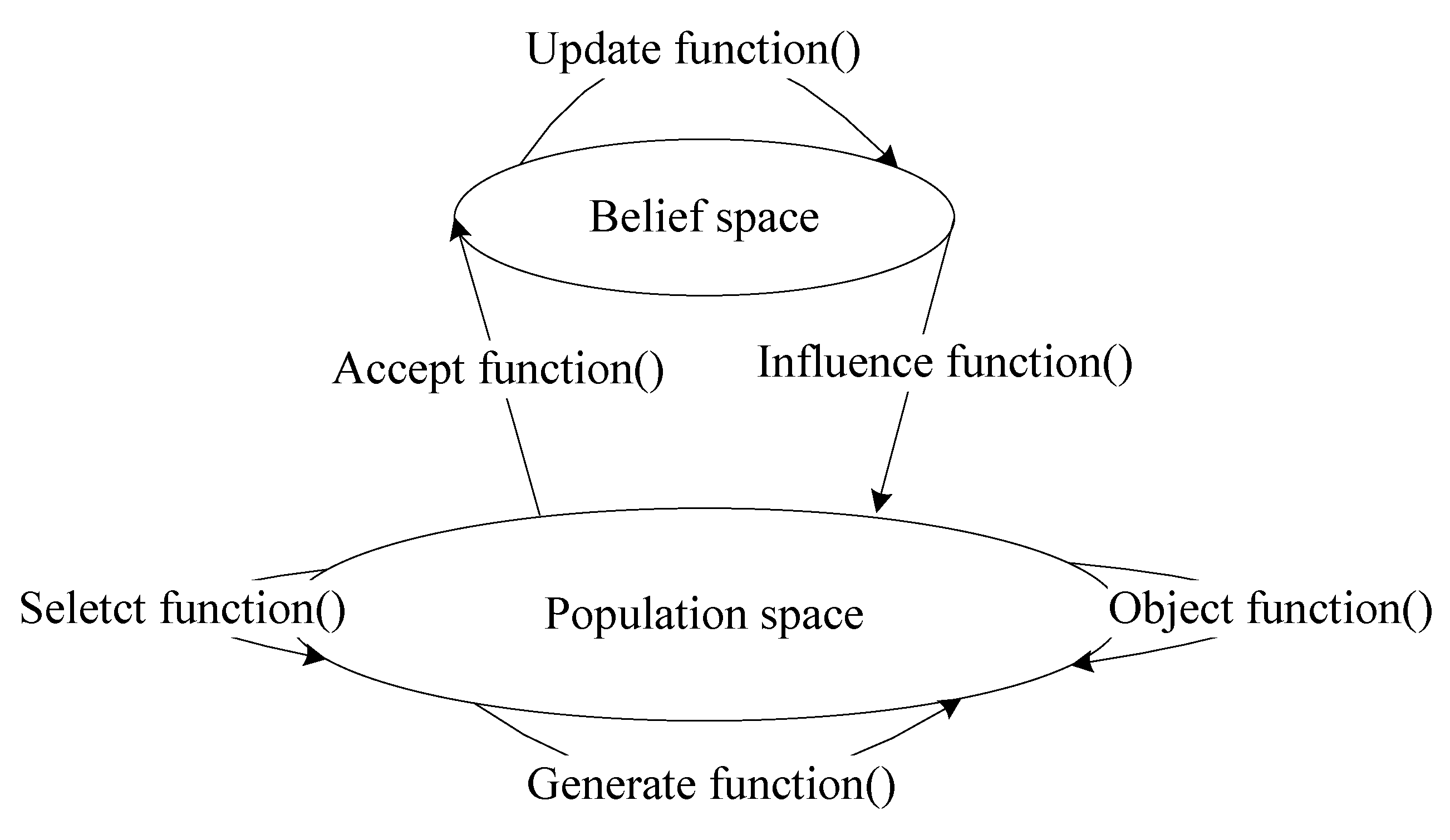
Cultural algorithms (CAs) are inspired by the processes of cultural evolution that occur in the natural world. The effectiveness of the CA framework has already been established in many applications. Figure 2 illustrates the general architecture of a CA. A CA consists of a population space (POP) and a belief space (BLF). POP and BLF have independent evolution processes. In a CA, these spaces are connected by a communication protocol, i.e., a functional function, which enables these spaces to cooperatively drive the evolution and optimization of the individuals in the population. The functional functions of a CA are the “accept function” and “influence function”.
As CAs possess many evolutionary processes, a different hybrid cultural algorithm can be developed by including a different evolutionary algorithm in the POP space. Theoretically, any evolutionary algorithm can be incorporated within the POP space as an evolutionary rule. However, a systematic theoretical foundation has yet to be established for applying CAs as an intelligent optimization algorithm.

3. Cultural-Algorithm-Based Evolutionary Multilabel Classification Algorithm

3.1. Weighted Bayes Multilabel Classification Algorithm

In Assumption A of the NBMLC algorithm, all the attribute nodes exhibit an equal level of importance for the selection of a class label node. In single-label problems, many researchers incorporate feature weighting in the NBMLC algorithm to correct this assumption. This has been demonstrated to improve classification accuracy [26,60,61]. In this work, we apply the weighting approach to the multilabel classification problem and, thus, obtain the weighted naïve Bayes multilabel classifier (WNBMLC). Here, wj represents the weight of the attribute xj, i.e., the importance of xj for the class label set. Equation (1) shows the mathematical expression of the WNBMLC algorithm.
P ( C i | X ) = arg max C i P ( C i ) j = 1 d P ( x j | C i ) w j
Here, it is illustrated that the key to solving the multilabel classification problem lies in the weighting of sample features. First, we constructed a WNBMLC (see Figure 3), where the nodes C1 and C2 correspond to the class attributes C1 and C2. The nodes A1, A2, A3, and A4 represent the four attributes, A1, A2, A3, and A4. The class nodes C1 and C2 are the parent nodes of the attribute nodes A1, A2, A3, and A4. The weights of the conditional attributes A1, A2, A3, and A4 for the selection of a class label from the class label set C = {C1, C2} are w1, w2, w3, and w4, respectively. In this work, a CA was used to iteratively optimize the selection of feature weights.

3.1.1. Correction of the Prior Probability Formula

An NBC occasionally calculates probabilities that are zero or very close to zero. Therefore, it is necessary to consider cases where the denominator becomes zero and to prevent underflows caused by the multiplication of small probabilities. Furthermore, while calculating conditional probabilities, an extreme situation can occasionally arise where all the training instances either belong to or do not belong to a class label. Thereby, the class label has a value of one or zero, respectively. This can occur if there are very few samples in the training set or when the dimensionalities of the attributes and class labels are very large. Consequently, the sample instances in the training set do not fully cover the relationship between the attributes and class labels, and it becomes infeasible to classify the records of the test set using the NBC. For example, it is feasible for the training set class label C1 = 1 to have a probability of zero. The denominator then becomes zero in the equations for calculating the average and variance of the conditional probability, resulting in erroneous calculations. We circumvented this problem by using the M-estimate while calculating prior probabilities. Equation (2) shows the definition of the M-estimate.
P ( X i | Y j ) = n c + m × p n + m
In this equation, n is the total number of instances that belong to the class label Yj in the training set; nc is the number of sample instances in the training set that belong to the class label Yj and have an attribute value of Xi; m is a deterministic parameter called the equivalent sample size; p is a self-defined parameter. According to this equation, if the training set is absent or the number of sample instances in the training set is zero, nc = n = 0, and P (Xi | Yj) = p. Therefore, p may be considered the prior probability for the appearance of the attribute Xi in the class Yj. In addition, prior probability (p) and observation probability (nc/n) are determined by the equivalent sample size (m). In this work, m is defined as one, and the value of p is 1/|C|, where |C| is the total number of class labels, i.e., the dimensionality of the class label set. Therefore, Equation (3) shows the equation for calculating prior probability.
P ( C i ) = | C i , D | + 1 / | C | | D | + 1

3.1.2. Correction of the Conditional Probability Formula

Correction for Assumption A in the conditional probability formula: Suppose that the instances of the training set adhere to a Gaussian density function. If all the training set instances belong to (or do not belong to) a certain class label, the number of elements in the average and variance formulae that correspond to the class label will be zero. Therefore, the denominator becomes zero. In this scenario, the calculated conditional probabilities are meaningless. In this work, it is assumed that for each class label, there is a minimum of one instance in the training set that belongs to that class label and also a minimum of one instance in the training set that does not belong to that class label. Therefore, if a class label was not selected in the sample instances of a training set, the algorithm will still assume that it was selected in one instance. This does not affect the results of the classification because it is a low-probability event compared to the number of training set instances. However, it ensures that the denominator in the conditional probability formula will not become zero. That is, regardless of the number of sample instances wherein a class label was evaluated as zero under a certain specified set of conditions, the selection count will always be incremented by one to ensure that this class label is selected in a minimum of one instance or not selected in one instance.
Correction for Assumption B: Suppose that conditional probability is being calculated by discretizing the continuous attribute values. If all the sample instances of a training set belong to (or do not belong to) a class label, Nj (Ck) = 0. Therefore, the denominator of P ( x i , j | C k ) = N j , n ( C k ) N j ( C k ) becomes zero. This data would then be considered invalid by the classifier. To resolve this issue, we used the M-estimate to smooth the conditional probability formula, as in Equation (4).
P ( x i , j | C k )   =   N j , n ( C k ) + 1 / ( | A j | ) N j ( C k ) + 1

3.1.3. Correction of the Posterior Probability Formula

In this work, the logarithm summation (log-sum) method was used to prevent underflows caused by the multiplication of small probabilities. In   P ( X | C i ) = P ( x 1 , x 2 , , x n ) = k = 1 n P ( x k | C i ) , even if all of the factors in the multiplication product are not zero, if n is large, the final result of P ( X | C i ) can be zero, or an underflow may occur and prevent the evaluation of P ( X | C i ) . In this scenario, it is infeasible to classify the test samples via stringent pairwise probability comparisons. It is, therefore, necessary to convert the probabilities through Equations (5) and (6).
P ( X | C i ) P ( C i ) = P ( C i ) k = 1 n P ( x k | C i )
log P ( X | C i ) = log ( P ( C i ) k = 1 n P ( x k | C i ) ) = log P ( C i ) + k = 1 n log ( P ( x k | C i ) )
The product calculation is transformed into a log-sum to solve this problem. This solves the underflow problem effectively, improves the accuracy of the calculation, and facilitates stringent pairwise comparisons. To ensure accurate calculations in this work, M-estimate-smoothed equations were used to calculate prior probability and conditional probability, whereas the log-sum method was used to calculate posterior probability in all the experiments described in this paper.

3.2. Improved Cultural Algorithm

In the proposed algorithm, the individuals (chromosomes) in the POP space are designed using real-number coding. The variables of the individuals are randomly initialized in the (0.0, 1.0) range of real numbers so that each chromosome consists of a set of real numbers. The dimensionality of the chromosome is equal to the dimensionality of the conditional attributes in the sample data. Moreover, each real number corresponds to a conditional attribute in the dataset. Suppose that the population size is N and that the attribute dimensionality of an individual in the population is n. Then, each individual in the population, Wi, may be expressed as an n-dimensional vector such that Wi = {w1, w2, …, wj, … wn}. In this equation, wj is the weight of the j-th attribute of individual wi, which is within (0.0, 1.0). The structure of each chromosome is shown in Figure 4.
Here, wi∊(0,1), and n represents the dimensionality of the conditional attributes in the multilabel classification problem.
The structure of the POP space is shown in Figure 5.

3.2.1. Definition and Update Rules of the Belief Space

The BLF space in our algorithm uses the <S, N> structure. Here, S is situational knowledge (SK), which is mainly used to record the exemplar individuals in the evolutionary process. The structure of SK may be expressed as SK = {S1, S2, …, SS}. In this equation, S represents the capacity of SK, and the structure of each individual in the SK set has the expression Si = {xji | f (Si)}. In this equation, Si is the i-th exemplar individual in the SK set, and f(xi) is the fitness of individual xi in the population. The structure of SK is shown in Figure 6, and the update rules for SK are shown in Equation (7).
s t + 1 = { x b e s t t f ( x b e s t t ) > f ( s t ) s t o t h e r s
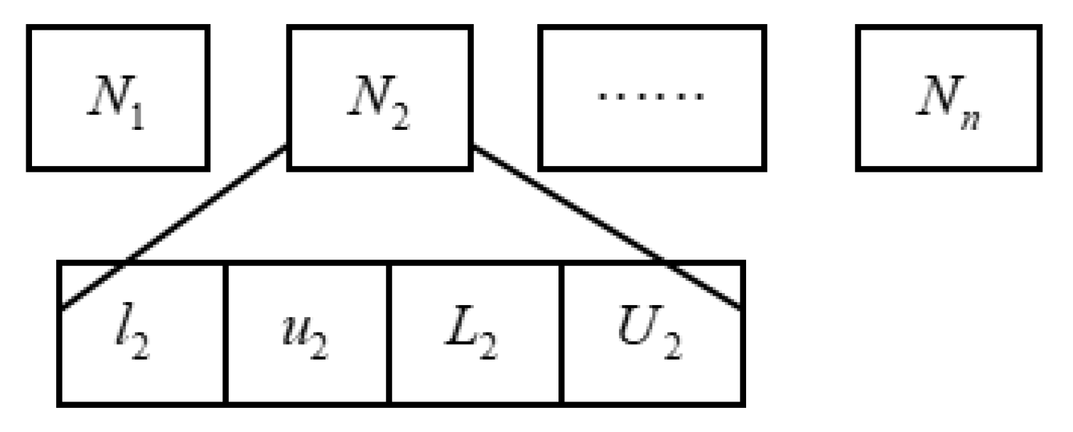
N is normative knowledge (NK). In the BLF space, it is the information that is effectively carried by the range of values of the variable. When a CA is used to optimize a problem of dimensionality n, the expression of NK is NK = {N1, N2, …, Nn}. In this equation, Ni = {(li, ui), (Li, Ui)}. Here, in, and li and ui are the lower and upper limits of the i-th dimensional variable, which are initialized as zero and one, respectively. Li and Ui are the individual fitness values that correspond to the li lower limit and ui upper limit, respectively, of variable xi. Li and Ui are initialized as positively infinite values. The structure of NK is shown in Figure 7, and the update rules for NK are shown in Equation (8).
l i t + 1 = { x j , i x j , i < = l i t   o r   f ( x j ) < L i t l i t o t h e r s L i t + 1 = { f ( x j ) x j , i < = l i t   o r   f ( x j ) < L i t L i t o t h e r s u i t + 1 = { x k , j x k , i > = u i t   o r   f ( x k ) > U i t u i t o t h e r s U i t + 1 = { f ( x k ) x k , i > = u i t   o r   f ( x k ) > U i t U i t o t h e r s

3.2.2. Fitness Function

In this work, the fitness function is defined as the accuracy of the class labels predicted by the algorithm. Therefore, the value of the fitness function of the t-th generation of the i-th individual, f(Xit), is equal to the classification accuracy that is obtained by substituting the weight of individual Xit into the weighted naïve Bayes posterior probability formula. Therefore, substituting the weight of the dimension corresponding to individual Xit into the weighted naïve Bayes posterior probability formula (Equations (1)–(3)) yields the theoretical class label. This theoretical class label, Jidk, is then compared to the real class label, Ji k. A score of one is assigned if they are equal, and zero otherwise. If there are n test instances and m class label dimensions, the equation for calculating the fitness of an individual is shown in Equation (9).
f ( X i t ) = i = 1 n k = 1 m ( J i , k d J i , k ) n m

3.2.3. Influence Function

The influence function (Equation (10)) is the channel by which the BLF space guides the evolution of individuals in the POP space. That is, the influence function enables the various knowledge categories of the BLF space to influence the evolution of individuals in the POP space. To adapt the CA to the multilabel classification problem, NK was used to adjust the step-length of the individuals’ evolution. Meanwhile, SK was used to direct the evolution of the individuals.
x j , i t + 1 = { x j , i t + | s i z e ( I i ) N ( 0 , 1 ) | x j , i t < s i t x j , i t | s i z e ( I i ) N ( 0 , 1 ) | x j , i t > s i t x j , i t + s i z e ( I i ) N ( 0 , 1 )       x j , i t = s i t

3.2.4. Selection Function

In the CA-based weighted naïve Bayes multilabel classification (CA-WNB) algorithm, the greedy search strategy is used to determine whether a newly generated test individual, vj,i(t + 1), will replace the parent individual in the t-th generation, xj,i(t), to form a new individual in the t + 1-st generation, xj,i(t + 1). The algorithm compares the fitness value of vj,i(t + 1), f(vj,i(t + 1)) to that of xj,i(t), f(xj,i(t)). vj,i(t + 1) will be selected for the next generation only if f(vj,i(t + 1)) is strictly superior to f(xj,i(t)). Otherwise, xj,i(t) will be retained in the t + 1-th generation. This approach systematically selects superior individuals for retention in the next generation. The implementation of this approach can be mathematically expressed as Equation (11).
x i ( t + 1 ) = { v j , i ( t + 1 ) , i f   f ( v j , i ( t + 1 ) ) > f ( x j , i ( t ) ) x j , i ( t ) , o t h e r s
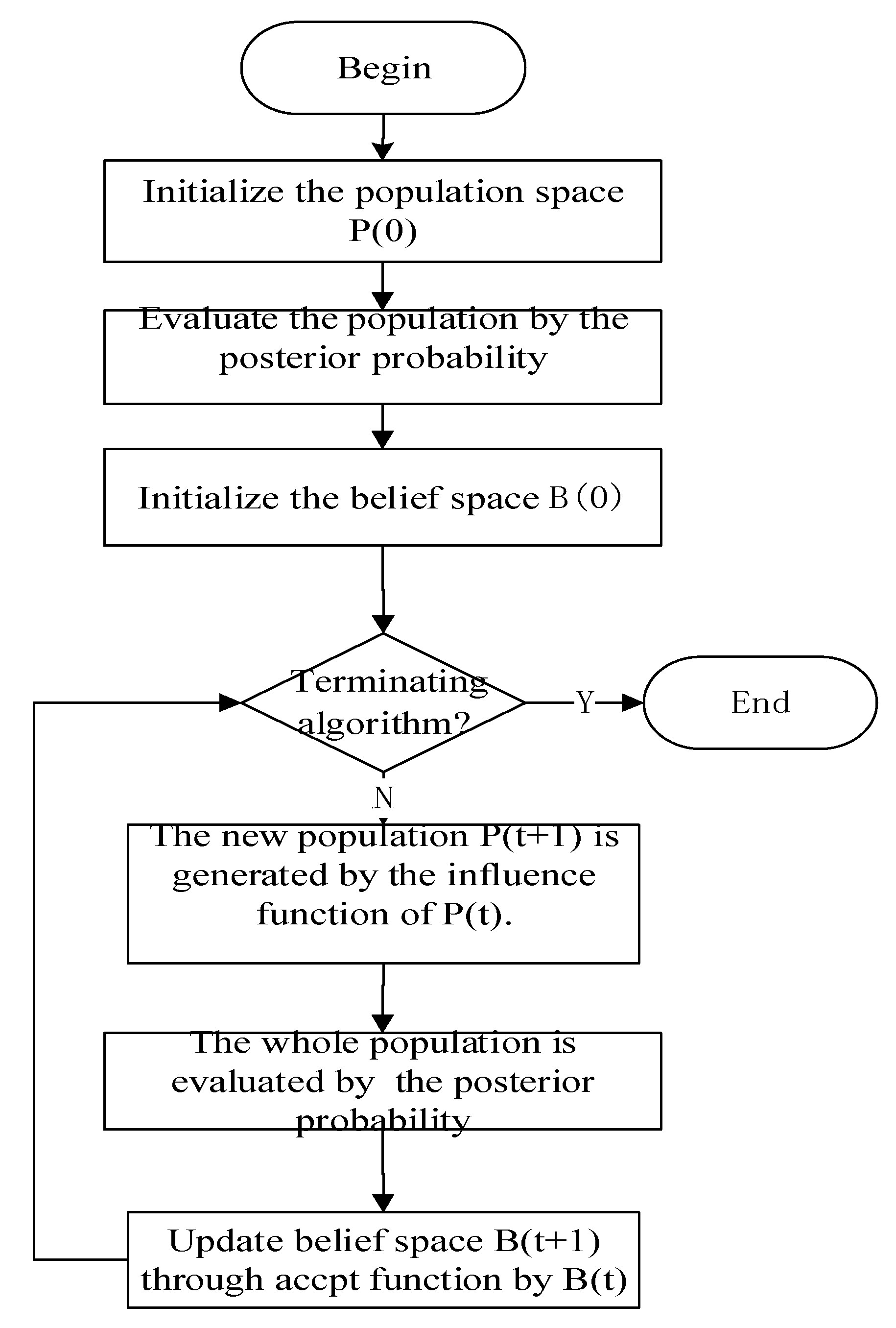
The process of our improved CA is shown in Figure 8:

3.3. CA-Based Evolutionary Multilabel Classification Algorithm

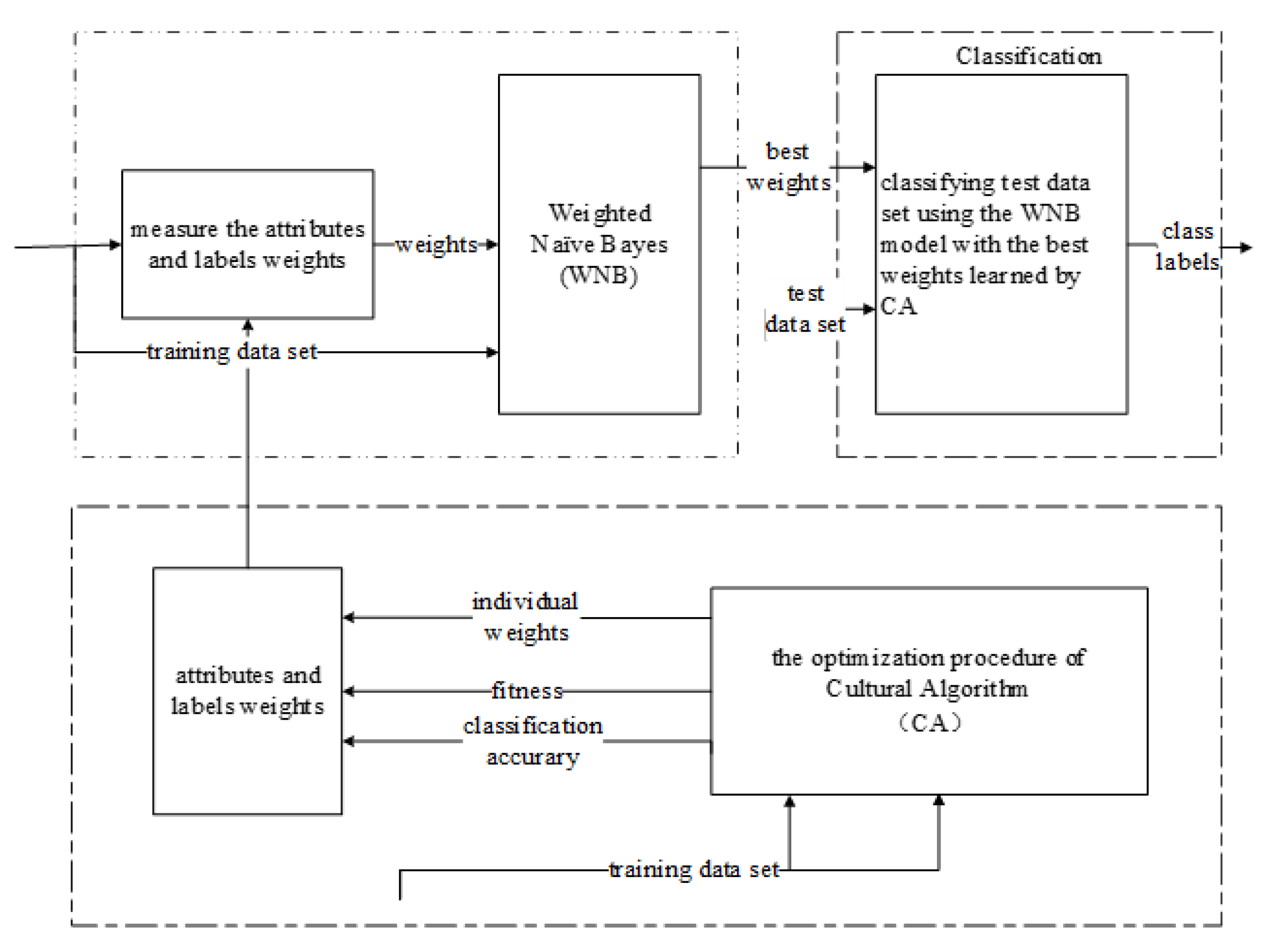
In the CA-WNB algorithm, the main purpose of the CA is to determine the weight of the attributes for label selection as the weight searching process is effectively a label-learning process. Once the optimal weights have been determined, the attribute weights may be used to classify the test set’s instances. The architecture of the CA-WNB algorithm is shown in Figure 9. The procedure of the CA-WNB algorithm is described below. It provides a detailed explanation of the algorithm’s architecture. The training of the CA-WNB algorithm is performed according to the following procedure:
Step 1: The data is preprocessed using stratified sampling. In this step, 70% of the sample dataset is randomly imported into the training set. The other 30% of the dataset is imported into the test set. The prior and posterior probabilities of the sample data in the training set (with M-estimate smoothing applied) are then calculated.
Step 2: Initialize the POP space. The individuals in the POP are randomly initialized, with each individual corresponding to a set of feature weights. The size of the population is NP.
Step 3: Evaluate the POP. Let wi = xi. In addition, normalize wi (the sum of all the attribute weights should be equal to one so that the sum of all the variables in the chromosome is one). The weights of each individual are substituted into the weighted naïve Bayes posterior probability formula (which uses the log-sum method) to predict the class labels of the sample data in the training set. The resulting classification accuracies are then considered the fitness values of the individuals. The evaluation of the POP space is thus completed, and the best individual in the POP is stored.
Step 4: Initialize the BLF. NK and SK are obtained by selecting the range of the BLF according to the settings of the accept function and the individuals in this range.
Step 5: Update the POP. Based on the features of NK and SK of the BLF, new individuals are generated in the POP according to the influence rules of the influence function. In the selection function, the exemplar individuals are selected from the parents and children according to the greedy selection rules, thus forming the next generation of the POP.
Step 6: Update the BLF. If the new individuals are superior to the individuals of the BLF, the BLF is updated. Otherwise, Step 5 is repeated until the algorithm attains the maximum number of iterations or until the results have converged. The algorithm is then terminated.
CA optimization is used to obtain the optimal combination of weights based on the training set. The weighted naïve Bayes posterior probability formula is then used to predict the class labels of the unlabeled test set instances. The predictions are then scored: a point is scored if the prediction is equal to the theoretical value; no point is scored otherwise. This ultimately yields the average classification accuracy of the test set’s instances.

4. Experimental Results and Analysis

4.1. Experimental Datasets

In most cases, the efficacy of multilabel classification is strongly correlated with the characteristics of the dataset. A few of these datasets may have gaps, noise, or nonuniform distributions. The dataset’s attributes may also be strongly correlated. Moreover, the data may be discrete, continuous, or a mix of both. The datasets used in this work have been normalized. That is, the attribute data have been scaled so that their values fall within a small, specified value interval, which is generally 0.0–1.0.
Single instance multilabel datasets were selected for this experiment. In datasets of this type, a task can be represented by an instance. However, this instance belongs to multiple class labels simultaneously. Given a multilabel dataset D and class label set C = {C1, C2, C3, C4}, if there is a tuple, Xi, whose class labels are Yi = {C1, C3}, the sample instance is represented as {Xi |1, 0, 1, 0}. That is, all the sample instances in the dataset must include all the labels in the label set. If an instance belongs to the class label Ci, the value of Ci is one; if an instance does not belong to Ci, the value of Ci is zero.
As the proposed multilabel classification algorithm is mainly aimed at text data, to ensure that the results of the validation experiments are universally comparable, the simulation experiments were performed using four widely accepted and preprocessed multi-label datasets that were obtained from the following multilabel datasets website: http://mulan.sourceforge.net/datasets.html, accessed on 16 February 2021. The CAL500 and emotions datasets concern music and emotion, the yeast dataset is from bioinformatics, and the scene dataset comprises natural scenes; the features of these datasets are described in Table 2.

4.2. Classification Evaluation Criteria

Multilabel data are generally mined to achieve two objectives: to classify multilabel data and to sort large numbers of labels. In this work, we focus only on multilabel classification. Therefore, the evaluation criteria used in this work are based on evaluation criteria for classification methods. According to the characteristics of the experimental data, if we suppose that there is a multilabel dataset D, a class label set C = {C1, C2, C3, C4}, and a Xi tuple whose class labels are Yi = {C1, C3}, the representation of the sample instance is then {Xi | 1, 0, 1, 0}. In a multilabel classification problem, the label set, Zi, that was predicted by the multilabel classifier for Xi may differ from the actual label set, Yi. Suppose that the class label set that was obtained by the algorithm is {1, 0, 0, 0}. As this set partially matches the real set, {1, 0, 1, 0}, the prediction accuracy of this instance is Accuracyi = (3/4) × 100% = 75%. That is, three of the four class labels were predicted correctly. Each correct prediction results in 1 point while a wrong prediction results in 0 points; prediction accuracy is given by the number of points divided by the dimensionality of the class label set. It is thus shown that the prediction accuracy of each test instance ranges within [0, 1]. If F( C i k ) and C i k represent the theoretical (i.e., algorithm-predicted) and real values, respectively, of the class label in the k-th dimension of the i-th sample instance in the test set, then N is the total number of sample instances in the test set and m is the dimensionality of the class label set. The equation for calculating the classification accuracy of each to-be-classified sample instance in the test set is Equation (12).
Accurac y i = 1 m k=1 m T( F( C i k ), C i k )
The T (F( C i k ), C i k ) function returns a value of one if the values of F( C i k ) and C i k are equal, and zero otherwise, as per Equation (13).
T ( F ( C i k ) , C i k ) = { 1 F ( C i k ) = C i k 0 F ( C i k ) C i k
The average criterion of the algorithm is the average classification accuracy of all the sample instances in the test set. It is calculated using Equation (14).
A c c u r a c y = 1 N i = 1 N 1 m k = 1 m T ( F ( C i k ) , C i k )

4.3. Classification Prediction Methods

CA produces a set of feature weights at the end of its iteration. The two classification methods described in [31] is used to predict the classification accuracy of each individual for the test sets. As these algorithms use topological rankings to predict an algorithm’s classification accuracy, the population size (NP) of the CA must be at least 30 to ensure that these algorithm prediction methods remain effective.

4.4. Analysis of the Results of the NBMLC Experiment

In the NBMLC experiment, stratified sampling was used to randomly import 70% of the sample instances into the training set. The remaining 30% of the samples were imported into the test set. The attributes of the experimental datasets are continuous, and there are many methods by which an NBC can compute their conditional probabilities. Therefore, three common fitting methods (Gaussian distribution, Cauchy distribution, and data discretization) were used in the experimental validation. The calculated results were then compared to analyze the strengths and weaknesses of each fitting method. In the data discretization experiment, data fitting was performed by specifying the initial number of discrete intervals, which is 10 in this experiment. Ten independent trials were then performed by applying the NBMLC algorithm to each of the four experimental datasets. The maximum (MAX), minimum (MIN), and average (AVE) values of the 10 trials were then recorded. The experimental results are presented in Table 3.
The analysis of the results of the three fitting experiments is presented in Table 4. In this table, Gau-Cau represents the difference between the average classification accuracies of the Gaussian and Cauchy distribution experiments. Dis-Gau represents the difference between the average classification accuracies of the data discretization experiment and the Gaussian distribution experiment. Dis-Cau is the difference between the average classification accuracies of the data discretization experiment and the Cauchy distribution experiment.
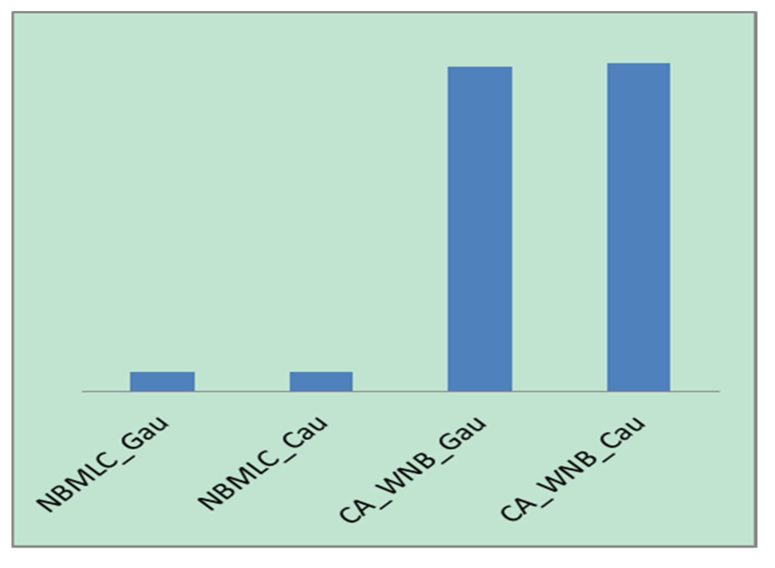
All three fitting methods exhibit a time complexity of magnitude O(N × n × m). Here, N is the size of the dataset, n the dimensionality of the attributes, and m the dimensionality of the class labels. Figure 10 shows the total computation times of each distribution method in their 10 trial runs, which were performed using identical computational hardware. The horizontal axis indicates the type of fitting method, whereas the vertical axis indicates the computation time consumed by each method.
Table 4 compares the classification accuracies of the NBMLCs with three distribution methods. It is demonstrated that the classification accuracy of an NBMLC is the highest when data discretization is used to fit the conditional probabilities. Furthermore, it is demonstrated that the data discretization approach yields higher classification efficacy in highly concentrated datasets. The use of Gaussian and Cauchy distributions to fit the conditional probabilities of the dataset resulted in significantly poorer results than that of the discretization approach. Furthermore, the classification accuracies obtained with Gaussian and Cauchy distribution are similar. Further analysis revealed that the effects of the different distribution methods on classification accuracy are significantly more pronounced in the “emotions” dataset than in the CAL500, “scene”, or “yeast” datasets. In the “emotions” dataset, the classification accuracy of the discretization approach is nearly 13% higher than that of the other approaches. In the “scene”, “yeast”, and CAL500 datasets, the discretization approach outperformed the other approaches by 4%, 3%, and 1%, respectively. An analysis of the characteristics of the datasets revealed that the class label dimensionality of the “emotions” dataset is smaller than that of the other datasets. It is followed by the “scene” dataset and the “yeast” dataset. The CAL500 dataset had the highest number of class label dimensions. Therefore, it may be concluded that the classification accuracies of these fitting methods become more similar as the number of class label dimensions increase. Although the algorithmic time complexities of these fitting methods are on an identical level of magnitude, the attribute values of the test data must be divided into intervals in the discretization approach. This requirement resulted in higher computation times than the Gaussian and Cauchy distribution approaches.

4.5. Analysis of Results of the CA-WNB Experiment

In the CA-WNB algorithm, there are three parameters that are relevant for the CA: the maximum number of iterations, population size, and the initial acceptance ratio of the accept function. The configuration of these parameters is presented in Table 5.
In the CA-WNB algorithm, the CA is used to optimize the attribute weights of the WNBMLC and to validate the weights of the three methods for conditional probability fitting. The results obtained by the CA-WNB algorithm were compared to those by the ordinary NBMLC algorithm, based on the abovementioned design rules and experimental evaluation criteria for classification functions. As the Gaussian and Cauchy approaches attempt to model the continuous attributes of each dataset by fitting their probability curves, and the NBMLC results associated with these approaches are similar, we used Prediction Methods 1 and 2 to compare the experimental results corresponding to the CA-WNB and NBMLC algorithms with Gaussian and Cauchy fitting. These comparisons were also conducted between the CA-WNB and NBMLC algorithms with the discretization approach, with varying numbers of discretization intervals (num = 10 and num = 20).

Gaussian and Cauchy Distribution

Table 6 [62] shows the experimental results of the best individuals produced by the CA-WNB and NBMLC algorithms with Gaussian and Cauchy distribution, according to Prediction Methods 1 and 2. The CA-WNB and NBMLC algorithms were applied to four experimental datasets, and 10 trials were performed for each dataset. The MAX, MIN, and AVE of these trials were then recorded. In Table 6, CA-WNB-P1 and CA-WNB-P2 represent the classification accuracies predicted by Prediction Methods 1 and 2, respectively, for the individuals produced by the CA-WNB algorithm.
Table 7, Table 8 and Table 9 [31] compare the experimental results of the top-10, top-20, and top-30 topological rankings of Prediction Methods 1 and 2 between the individuals produced by the CA-WNB and NBMLC algorithms with Gaussian and Cauchy distribution.
Table 10 and Table 11 present the average classification accuracy of the weighting combinations corresponding to the final-generation individuals whose fitness values ranked in the top-10, top-20, and top-30, as yielded by Prediction Methods 1 and 2, in the classification of the four experimental datasets; Gaussian and Cauchy distribution were used to model conditional probability. These tables also show the percentage by which the CA-WNB algorithm improves upon the classification accuracies of the NBMLC algorithm, according to Prediction Methods 1 and 2. The bolded entries in these tables indicate the classification accuracy obtained by the best individual. The bottom rows of these tables present the average classification accuracy of the three algorithms. CA-WNB-P1 and CA-WNB-P2 are the average classification accuracies obtained using the CA-WNB algorithm, according to Prediction Methods 1 and 2.
It is apparent that the average accuracy obtained by the CA-WNB algorithm is superior to that of the NBMLC algorithm. However, this is obtained at the expense of computation time. The CA-WNB algorithm iteratively optimizes attribute weights prior to the prediction of class labels so as to weaken the effects of the naïve conditional independence assumption. Even if one overlooks the effects of having multiple prediction methods and different training and test dataset sizes on the computation time, the time complexity of the CA-WNB algorithm is still NP × MAXGEN times higher than that of the NBMLC algorithm (NP is the population size, and MAXGEN is the maximum number of evolutions). The running times of the CA-WNB and NBMLC algorithms (under the same conditions and environment as in the abovementioned experiments) are shown in Figure 11. NBMLC-Gau and NBMLC-Cau are the running times of the NBMLC algorithm with Gaussian and Cauchy distribution, respectively. Meanwhile, CA-WNB-Gau and CA-WNB-Cau are the running times of the CA-WNB algorithm with Gaussian and Cauchy distribution, respectively.
The experimental results demonstrate the following:
(1)
Based on Figure 11, the CA-WNB algorithm consumes a significantly longer computation time than the NBMLC algorithm.
(2)
If one omits computational cost, the CA-WNB algorithm is evidently superior to the simple NBMLC algorithm in terms of classification performance. The percentage improvement in classification accuracy with the CA-WNB algorithm was most pronounced in the “emotions” dataset, followed by the “scene”, “yeast”, and CAL500 datasets. An analysis of the characteristics of these datasets revealed that the use of stratified sampling to disrupt the “emotions” and “scene” datasets did not significantly affect their classification accuracies. Meanwhile, the effects of this operation on the CAL500 and “yeast” datasets are more pronounced. This illustrates that the “emotions” and “scene” datasets have relatively uniform distributions of data, whereas the CAL500 and “yeast” datasets have highly nonuniform data distributions. If the training dataset is strongly representative of the dataset, the classification efficacy of the algorithm will be substantially improved by the training process. Otherwise, the improvement in classification efficacy will not be very significant. Based on this observation, weighted naïve Bayes can be used to optimize classification efficacy if the distribution of the dataset is relatively uniform and if the time requirements of the experiment are not particularly stringent.
(3)
A comparison of Table 10 and Table 11 reveals that the improvement in the average classification accuracy yielded by Prediction Method 2 (6.79% and 7.43%) is always higher than that yielded by Prediction Method 1 (6.54% and 7.20%) regardless of whether Gaussian or Cauchy fitting is used. Furthermore, the improvement in average classification accuracy is always higher with the Gaussian fitting (7.20% and 7.43%) than with the Cauchy fitting (6.54% and 6.79%). A comparison of the results with Cauchy fitting and Gaussian fitting reveals that the results of the CA-WNB algorithm with Cauchy fitting varied substantially. Moreover, the weights obtained by the CA also exert a higher impact on the Cauchy fitting. Therefore, the results with Cauchy fitting are unstable to a certain degree. Nonetheless, the average classification accuracy of the CA-WNB algorithm with Cauchy fitting is superior to that of the CA-WNB algorithm with Gaussian fitting.
(4)
Table 10 and Table 11 reveal that the highest average classification accuracies for the four experimental datasets were obtained by individuals with Ranks 10–20, according to Prediction Method 2. Conversely, the worst classification accuracies were obtained by individuals with Ranks 20–30. It is established that the weights that have the best fit with training set instances may not be the optimal weights for classifying test set instances. After a certain number of evolutions in the population, excessive fitting may have occurred because the fitting curves were adjusted too finely, thereby resulting in less-than-ideal classification accuracies for the test set’s instances. Consequently, the fitting curves produced by the weights of individuals with Ranks 10–20 were better for classifying the instances of the test set.

5. Conclusions

In this paper, we study the multilabel classification problem. This paper presents the algorithm framework of naïve Bayes multilabel classification and analyzes and compares the effects of three common fitting methods of continuous attributes on the classification performance of the naïve Bayes multilabel classification algorithm from the perspective of average classification accuracy and algorithm time cost. On this basis, the framework of weighted naïve Bayes multilabel classification is given, the determination of weights is regarded as an optimization problem, the cultural algorithm is introduced to search for and determine the optimal weight, and the weighted naïve Bayes multilabel classification algorithm based on the cultural algorithm is proposed. In this algorithm, the classification accuracy obtained by substituting the current individual in the weighted naïve Bayes multilabel classification is taken as the objective function, and the attribute dimension represents the individual dimension. Each one-dimensional variable in the individual represents the weight of the corresponding dimension of the attribute, and the coding test and verification are carried out by real numbers to obtain a prediction strategy that is more suitable for the algorithm. Experimental results show that the algorithm proposed in this paper is superior to similar algorithms in classification performance when the time cost is not considered.

Author Contributions

Conceptualization, Q.W. and B.W.; Data curation, Q.W. and C.H.; Investigation, C.H.; Methodology, Q.W.; Software, C.H.; Visualization, X.Y.; Writing—original draft, Q.W.; Writing—review & editing, X.Y. All authors have read and agreed to the published version of the manuscript.

Funding

This research was funded by Natural Science Foundation of China (U1911205 and 62073300), the Fundamental Research Funds for the Central Universities, China University of 615 Geosciences (Wuhan) (CUGGC03) and the Fundamental Research Funds for the Central Univer-616 sities, JLU (93K172020K18).

Institutional Review Board Statement

Not applicable.

Informed Consent Statement

Not applicable.

Data Availability Statement

Not applicable.

Acknowledgments

This paper is supported by the Natural Science Foundation of China (U1911205 and 62073300), China University of Geosciences (Wuhan) (CUGGC03), and the Fundamental Research Funds for the Central Universities (JLU; 93K172020K18).

Conflicts of Interest

The authors declare no conflict of interest.

References

  1. Tsoumakas, G.; Katakis, I.; Vlahavas, I. Mining multi-label data. In Data Mining and Knowledge Discovery Handbook; Springer: Boston, MA, USA, 2010; pp. 667–685. [Google Scholar]
  2. Streich, A.P.; Buhmann, J.M. Classification of multi-labeled data: A generative approach. In Machine Learning and Knowledge Discovery in Databases; Springer: Berlin/Heidelberg, Germany, 2008; pp. 390–405. [Google Scholar]
  3. Kazawa, H.; Izumitani, T.; Taira, H.; Maeda, E. Maximal margin labeling for multi-topic text categorization. In Advances in Neural Information Processing Systems; MIT Press: Vancouver, BC, Canada, 2004; pp. 649–656. [Google Scholar]
  4. Snoek, C.G.; Worring, M.; Van Gemert, J.C.; Geusebroek, J.M.; Smeulders, A.W. The challenge problem for automated detection of 101 semantic concepts in multimedia. In Proceedings of the 14th annual ACM International Conference on Multimedia, Santa Barbara, CA, USA, 23–27 October 2006; ACM: New York, NY, USA, 2006; pp. 421–430. [Google Scholar]
  5. Vens, C.; Struyf, J.; Schietgat, L.; Džeroski, S.; Blockeel, H. Decision trees for hierarchical multi-label classification. Mach. Learn. 2008, 73, 185–214. [Google Scholar] [CrossRef] [Green Version]
  6. Boutell, M.R.; Luo, J.; Shen, X.; Brown, C.M. Learning multi-label scene classification. Pattern Recognit. 2004, 37, 1757–1771. [Google Scholar] [CrossRef] [Green Version]
  7. Xia, Y.; Chen, K.; Yang, Y. Multi-Label Classification with Weighted Classifier Selection and Stacked Ensemble. Inf. Sci. 2020. [Google Scholar] [CrossRef]
  8. Qian, W.; Xiong, C.; Wang, Y. A ranking-based feature selection for multi-label classification with fuzzy relative discernibility. Appl. Soft Comput. 2021, 102, 106995. [Google Scholar] [CrossRef]
  9. Yao, Y.; Li, Y.; Ye, Y.; Li, X. MLCE: A Multi-Label Crotch Ensemble Method for Multi-Label Classification. Int. J. Pattern Recognit. Artif. Intell. 2020. [Google Scholar] [CrossRef]
  10. Yang, B.; Tong, K.; Zhao, X.; Pang, S.; Chen, J. Multilabel Classification Using Low-Rank Decomposition. Discret. Dyn. Nat. Soc. 2020, 2020, 1–8. [Google Scholar] [CrossRef]
  11. Kumar, A.; Abhishek, K.; Kumar Singh, A.; Nerurkar, P.; Chandane, M.; Bhirud, S.; Busnel, Y. Multilabel classification of remote sensed satellite imagery. Trans. Emerg. Telecommun. Technol. 2020, 4, 118–133. [Google Scholar] [CrossRef]
  12. Huang, S.J.; Li, G.X.; Huang, W.Y.; Li, S.Y. Incremental Multi-Label Learning with Active Queries. J. Comput. Sci. Technol. 2020, 35, 234–246. [Google Scholar] [CrossRef]
  13. Zhang, M.L.; Peña, J.M.; Robles, V. Feature selection for multi-label naive Bayes classification. Inf. Sci. 2009, 179, 3218–3229. [Google Scholar] [CrossRef]
  14. De Carvalho, A.C.; Freitas, A.A. A tutorial on multi-label classification techniques. Found. Comput. Intell. 2009, 5, 177–195. [Google Scholar]
  15. Spyromitros, E.; Tsoumakas, G.; Vlahavas, I. An empirical study of lazy multilabel classification algorithms. In Artificial Intelligence: Theories, Models and Applications; Springer: Berlin/Heidelberg, Germany, 2008; pp. 401–406. [Google Scholar]
  16. Rousu, J.; Saunders, C.; Szedmak, S.; Shawe-Taylor, J. Kernel-based learning of hierarchical multilabel classification models. J. Mach. Learn. Res. 2006, 7, 1601–1626. [Google Scholar]
  17. Yang, Y.; Chute, C.G. An example-based mapping method for text categorization and retrieval. ACM Trans. Inf. Syst. (TOIS) 1994, 12, 252–277. [Google Scholar] [CrossRef]
  18. Grodzicki, R.; Mańdziuk, J.; Wang, L. Improved multilabel classification with neural networks. Parallel Probl. Solving Nat. Ppsn X 2008, 5199, 409–416. [Google Scholar]
  19. Gonçalves, E.C.; Freitas, A.A.; Plastino, A. A Survey of Genetic Algorithms for Multi-Label Classification. In Proceedings of the 2018 IEEE Congress on Evolutionary Computation (CEC), Rio de Janeiro, Brazil, 29 January 2018; pp. 1–8. [Google Scholar]
  20. McCallum, A.; Nigam, K. A comparison of event models for naive bayes text classification. AAAI-98 Workshop Learn. Text Categ. 1998, 752, 41–48. [Google Scholar]
  21. Gao, S.; Wu, W.; Lee, C.H.; Chua, T.S. A MFoM learning approach to robust multiclass multi-label text categorization. In Proceedings of the Twenty-First International Conference on Machine Learning; ACM: New York, NY, USA, 2004; pp. 329–336. [Google Scholar]
  22. Ghamrawi, N.; McCallum, A. Collective multi-label classification. In Proceedings of the 14th ACM International Conference on Information and Knowledge Management; ACM: New York, NY, USA, 2005; pp. 195–200. [Google Scholar]
  23. Zhang, M.L.; Zhou, Z.H. ML-KNN: A lazy learning approach to multi-label learning. Pattern Recognit. 2007, 40, 2038–2048. [Google Scholar] [CrossRef] [Green Version]
  24. Xu, X.S.; Jiang, Y.; Peng, L.; Xue, X.; Zhou, Z.H. Ensemble approach based on conditional random field for multi-label image and video annotation. In Proceedings of the 19th ACM International Conference on Multimedia; ACM: New York, NY, USA, 2011; pp. 1377–1380. [Google Scholar]
  25. Qu, G.; Zhang, H.; Hartrick, C.T. Multi-label classification with Bayes’ theorem. In Proceedings of the 2011 4th International Conference on Biomedical Engineering and Informatics (BMEI), Shanghai, China, 15–17 October 2011; pp. 2281–2285. [Google Scholar]
  26. Wu, J.; Cai, Z. Attribute weighting via differential evolution algorithm for attribute weighted naive bayes (wnb). J. Comput. Inf. Syst. 2011, 7, 1672–1679. [Google Scholar]
  27. Wu, J.; Cai, Z. A naive Bayes probability estimation model based on self-adaptive differential evolution. J. Intell. Inf. Syst. 2014, 42, 671–694. [Google Scholar] [CrossRef]
  28. Sucar, L.E.; Bielza, C.; Morales, E.F.; Hernandez-Leal, P.; Zaragoza, J.H.; Larrañaga, P. Multi-label classification with Bayesian network-based chain classifiers. Pattern Recognit. Lett. 2014, 41, 14–22. [Google Scholar] [CrossRef]
  29. Reyes, O.; Morell, C.; Ventura, S. Evolutionary feature weighting to improve the performance of multi-label lazy algorithms. Integr. Comput. Aided Eng. 2014, 21, 339–354. [Google Scholar] [CrossRef]
  30. Lee, J.; Kim, D.W. Memetic feature selection algorithm for multi-label classification. Inf. Sci. 2015, 293, 80–96. [Google Scholar] [CrossRef]
  31. Yan, X.; Wu, Q.; Sheng, V.S. A Double Weighted Naive Bayes with Niching Cultural Algorithm for Multi-Label Classification. Int. J. Pattern Recognit. Artif. Intell. 2016, 30, 1–23. [Google Scholar] [CrossRef]
  32. Wu, Q.; Liu, H.; Yan, X. Multi-label classification algorithm research based on swarm intelligence. Clust. Comput. 2016, 19, 2075–2085. [Google Scholar] [CrossRef]
  33. Zhang, Y.; Gong, D.W.; Sun, X.Y.; Guo, Y.N. A PSO-based multi-objective multi-label feature selection method in classification. Sci. Rep. 2017, 7, 376. [Google Scholar] [CrossRef] [PubMed]
  34. Wu, Q.; Wang, H.; Yan, X.; Liu, X. MapReduce-based adaptive random forest algorithm for multi-label classification. Neural Comput. Appl. 2019, 31, 8239–8252. [Google Scholar] [CrossRef]
  35. Moyano, J.M.; Gibaja, E.L.; Cios, K.J.; Ventura, S. An evolutionary approach to build ensembles of multi-label classifiers. Inf. Fusion 2019, 50, 168–180. [Google Scholar] [CrossRef]
  36. Guo, Y.N.; Zhang, P.; Cheng, J.; Wang, C.; Gong, D. Interval Multi-objective Quantum-inspired Cultural Algorithms. Neural Comput. Appl. 2018, 30, 709–722. [Google Scholar] [CrossRef]
  37. Yan, X.; Zhu, Z.; Hu, C.; Gong, W.; Wu, Q. Spark-based intelligent parameter inversion method for prestack seismic data. Neural Comput. Appl. 2019, 31, 4577–4593. [Google Scholar] [CrossRef]
  38. Wu, B.; Qian, C.; Ni, W.; Fan, S. The improvement of glowworm swarm optimization for continuous optimization problems. Expert Syst. Appl. 2012, 39, 6335–6342. [Google Scholar] [CrossRef]
  39. Lu, C.; Gao, L.; Li, X.; Zheng, J.; Gong, W. A multi-objective approach to welding shop scheduling for makespan, noise pollution and energy consumption. J. Clean. Prod. 2018, 196, 773–787. [Google Scholar] [CrossRef]
  40. Wu, Q.; Zhu, Z.; Yan, X.; Gong, W. An improved particle swarm optimization algorithm for AVO elastic parameter inversion problem. Concurr. Comput. Pract. Exp. 2019, 31, 1–16. [Google Scholar] [CrossRef]
  41. Yu, P.; Yan, X. Stock price prediction based on deep neural network. Neural Comput. Appl. 2020, 32, 1609–1628. [Google Scholar] [CrossRef]
  42. Gong, W.; Cai, Z. Parameter extraction of solar cell models using repaired adaptive differential evolution. Solar Energy 2013, 94, 209–220. [Google Scholar] [CrossRef]
  43. Wang, F.; Li, X.; Zhou, A.; Tang, K. An estimation of distribution algorhim for mixed-variable Newsvendor problems. IEEE Trans. Evol. Comput. 2020, 24, 479–493. [Google Scholar]
  44. Wang, G.G. Improving Metaheuristic Algorithms with Information Feedback Models. IEEE Trans. Cybern. 2017, 99, 1–14. [Google Scholar] [CrossRef] [PubMed]
  45. Yan, X.; Li, P.; Tang, K.; Gao, L.; Wang, L. Clonal Selection Based Intelligent Parameter Inversion Algorithm for Prestack Seismic Data. Inf. Sci. 2020, 517, 86–99. [Google Scholar] [CrossRef]
  46. Yan, X.; Yang, K.; Hu, C.; Gong, W. Pollution source positioning in a water supply network based on expensive optimization. Desalination Water Treat. 2018, 110, 308–318. [Google Scholar] [CrossRef] [Green Version]
  47. Wang, R.; Zhou, Z.; Ishibuchi, H.; Liao, T.; Zhang, T. Localized weighted sum method for many-objective optimization. IEEE Trans. Evol. Comput. 2018, 22, 3–18. [Google Scholar] [CrossRef]
  48. Lu, C.; Gao, L.; Yi, J. Grey wolf optimizer with cellular topological structure. Expert Syst. Appl. 2018, 107, 89–114. [Google Scholar] [CrossRef]
  49. Wang, F.; Zhang, H.; Zhou, A. A particle swarm optimization algorithm for mixed-variable optimization problems. Swarm Evol. Comput. 2021, 60, 100808. [Google Scholar] [CrossRef]
  50. Yan, X.; Zhao, J. Multimodal optimization problem in contamination source determination of water supply networks. Swarm Evol. Comput. 2019, 47, 66–71. [Google Scholar] [CrossRef]
  51. Yan, X.; Hu, C.; Sheng, V.S. Data-driven pollution source location algorithm in water quality monitoring sensor networks. Int. J. Bio-Inspir Compu. 2020, 15, 171–180. [Google Scholar] [CrossRef]
  52. Hu, C.; Dai, L.; Yan, X.; Gong, W.; Liu, X.; Wang, L. Modified NSGA-III for Sensor Placement in Water Distribution System. Inf. Sci. 2020, 509, 488–500. [Google Scholar] [CrossRef]
  53. Wang, R.; Li, G.; Ming, M.; Wu, G.; Wang, L. An efficient multi-objective model and algorithm for sizing a stand-alone hybrid renewable energy system. Energy 2017, 141, 2288–2299. [Google Scholar] [CrossRef]
  54. Li, S.; Gong, W.; Yan, X.; Hu, C.; Bai, D.; Wang, L. Parameter estimation of photovoltaic models with memetic adaptive differential evolution. Solar Energy 2019, 190, 465–474. [Google Scholar] [CrossRef]
  55. Yan, X.; Zhang, M.; Wu, Q. Big-Data-Driven Pre-Stack Seismic Intelligent Inversion. Inf. Sci. 2021, 549, 34–52. [Google Scholar] [CrossRef]
  56. Wang, F.; Li, Y.; Liao, F.; Yan, H. An ensemble learning based prediction strtegy for dynamic multi-objective optimization. Appl. Soft Comput. 2020, 96, 106592. [Google Scholar] [CrossRef]
  57. Yan, X.; Li, T.; Hu, C. Real-time localization of pollution source for urban water supply network in emergencies. Clust. Comput. 2019, 22, 5941–5954. [Google Scholar] [CrossRef]
  58. Reynolds, R.G. Cultural algorithms: Theory and applications. In New Ideas in Optimization; McGraw-Hill Ltd.: Berkshire, UK, 1999; pp. 367–378. [Google Scholar]
  59. Reynolds, R.G.; Zhu, S. Knowledge-based function optimization using fuzzy cultural algorithms with evolutionary programming. IEEE Trans. Syst. Man Cybern. Part B 2001, 31, 1–18. [Google Scholar] [CrossRef]
  60. Zhang, H.; Sheng, S. Learning weighted naïve Bayes with accurate ranking. In Proceedings of the 4th IEEE International Conference on Data Mining, Brighton, UK, 1–4 November 2004; pp. 567–570. [Google Scholar]
  61. Xie, T.; Liu, R.; Wei, Z. Improvement of the Fast Clustering Algorithm Improved by K-Means in the Big Data. Appl. Math. Nonlinear Sci. 2020, 5, 1–10. [Google Scholar] [CrossRef] [Green Version]
  62. Yan, X.; Li, W.; Wu, Q.; Sheng, V.S. A Double Weighted Naive Bayes for Multi-label Classification. In International Symposium on Computational Intelligence and Intelligent Systems; Springer: Singapore, 2015; pp. 382–389. [Google Scholar]
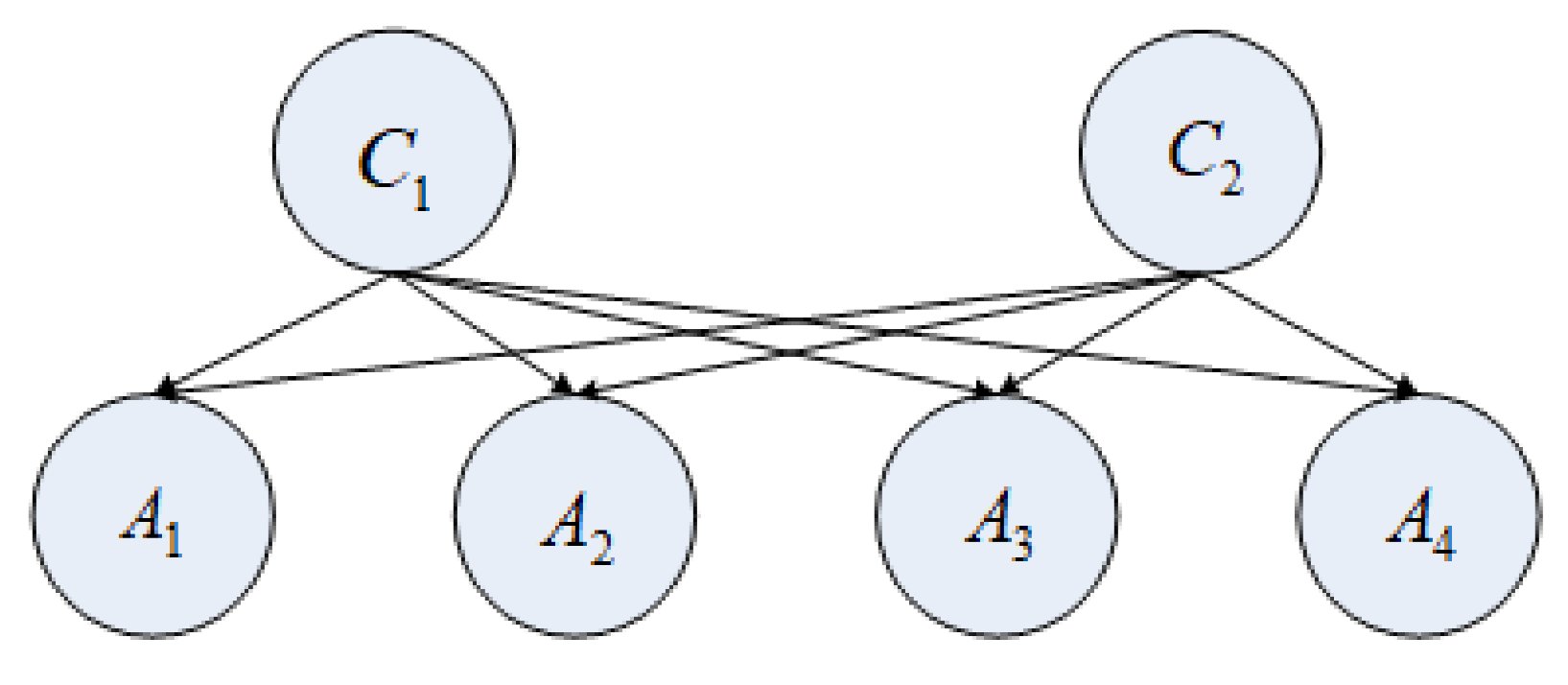
Figure 1. A naïve Bayes classifier.
Symmetry 13 00322 g001
Figure 2. Fundamental architecture of cultural algorithms.
Symmetry 13 00322 g002
Figure 3. Weighted naïve Bayes classifier.
Symmetry 13 00322 g003
Figure 4. Structure of a chromosome in the cultural algorithm.
Symmetry 13 00322 g004
Figure 5. Structure of the population space in the cultural algorithm.
Symmetry 13 00322 g005
Figure 6. Structure of situational knowledge.
Symmetry 13 00322 g006
Figure 7. Structure of normative knowledge.
Symmetry 13 00322 g007
Figure 8. Flowchart of the improved cultural algorithm.
Symmetry 13 00322 g008
Figure 9. Architecture of the cultural algorithm-based weighted naïve Bayes multilabel classification (CA-WNB) algorithm.
Symmetry 13 00322 g009
Figure 10. Comparison between the computational times of each of the three fitting methods.
Symmetry 13 00322 g010
Figure 11. Computation times of NBMLC and CA-WNB algorithms.
Symmetry 13 00322 g011
Table 1. Training dataset of a multilabel data model.
A 1 A 2 A 3 A 4 C 1 C 2
1 x 11 x 12 x 13 x 14 01
2 x 21 x 22 x 23 x 24 10
3 x 31 x 32 x 33 x 34 00
4 x 41 x 42 x 43 x 44 11
Table 2. The datasets used in this experiment.
Data SetDefinition DomainNo. of Samples in Sample SetNo. of AttributesNo. of Class Labels
Training SetTest SetNumerical TypeNoun Type
yeastBiology1500917103014
sceneImage1211119629406
emotionsMusic3912027206
CAL500Music351151680174
Table 3. Comparison between the results of the NBMLC experiment.
Data SetGaussianCauchyDisperse_10
MAXMINAVEMAXMINAVEMAXMINAVE
CAL5000.8732 0.8574 0.8622 0.8662 0.8588 0.8635 0.8838 0.8620 0.8740
emotions0.6976 0.6798 0.6884 0.7022 0.6798 0.6892 0.8361 0.7968 0.8168
scene0.8239 0.8195 0.8212 0.8241 0.8188 0.8151 0.8707 0.8552 0.8614
yeast0.7749 0.7636 0.7688 0.7720 0.7603 0.7673 0.8023 0.7799 0.7958
Table 4. Analysis of the results of the naïve Bayes multilabel classification (NBMLC) experiments.
Data SetGau-CauDis-GauDis-Cau
CAL500−0.00130.01180.0105
emotions−0.00080.12840.1276
scene0.00610.04020.0463
yeast0.00150.0270.0285
Table 5. Configuration of CA parameters.
ParameterPopulation SizeMaximum Number of IterationsInitial Acceptance Ratio
Value1002000.2
Table 6. Experimental results of NBMLC and CA-WNB for best value.
Data SetAlgorithmGaussianCauchy
MAXMINAVEMAXMINAVE
CAL_500NBMLC0.8732 0.8574 0.8622 0.8721 0.8554 0.8635
CA-WNB-P10.8893 0.8750 0.8813 0.8871 0.8737 0.8800
CA-WNB-P20.8897 0.87510.88250.8890 0.8744 0.8811
emotionsNBMLC0.6976 0.6798 0.6884 0.6976 0.6787 0.6892
CA-WNB-P10.8059 0.7853 0.7938 0.8215 0.7850 0.8040
CA-WNB-P20.8115 0.7900 0.79930.8215 0.7869 0.8044
sceneNBMLC0.8239 0.8195 0.8212 0.8195 0.8098 0.8151
CA-WNB-P10.8693 0.8564 0.8630 0.8841 0.8652 0.8732
CA-WNB-P20.8714 0.8592 0.86540.8848 0.8615 0.8744
yeastNBMLC0.7749 0.7636 0.7688 0.7739 0.7688 0.7673
CA-WNB-P10.8045 0.7787 0.7901 0.8129 0.7873 0.7948
CA-WNB-P20.8051 0.7851 0.79330.8126 0.7831 0.7952
Table 7. Experimental results of NBMLC and CA-WNB for top-10 value.
Data SetAlgorithmGaussianCauchy
MAXMINAVEMAXMINAVE
CAL_500NBMLC0.8732 0.8574 0.8622 0.8721 0.8554 0.8635
CA-WNB-P10.8885 0.8697 0.8821 0.8884 0.8727 0.8801
CA-WNB-P20.8897 0.8716 0.88290.8890 0.8744 0.8811
emotionsNBMLC0.6976 0.6798 0.6884 0.6976 0.6787 0.6892
CA-WNB-P10.8012 0.7799 0.7939 0.8224 0.7822 0.8039
CA-WNB-P20.8143 0.7900 0.80110.8271 0.7869 0.8070
sceneNBMLC0.8239 0.8195 0.8212 0.8195 0.8098 0.8151
CA-WNB-P10.8698 0.8592 0.8647 0.8836 0.8638 0.8725
CA-WNB-P20.8714 0.8592 0.86560.8848 0.8626 0.8746
yeastNBMLC0.7749 0.7636 0.7688 0.7739 0.7688 0.7673
CA-WNB-P10.8040 0.7898 0.79530.8115 0.7875 0.7943
CA-WNB-P20.8051 0.7851 0.7938 0.8126 0.7831 0.7941
Table 8. Experimental results of NBMLC and CA-WNB for top-20 value.
Data SetAlgorithmGaussianCauchy
MAXMINAVEMAXMINAVE
CAL_500NBMLC0.8732 0.8574 0.8622 0.8721 0.8554 0.8635
CA-WNB-P10.8884 0.8690 0.8823 0.8884 0.8740 0.8801
CA-WNB-P20.8903 0.8717 0.88320.8890 0.8744 0.8812
emotionsNBMLC0.6976 0.6798 0.6884 0.6976 0.6787 0.6892
CA-WNB-P10.8021 0.7843 0.7939 0.8231 0.7812 0.8071
CA-WNB-P20.8143 0.7900 0.80130.8271 0.7869 0.8088
sceneNBMLC0.8239 0.8195 0.8212 0.8195 0.8098 0.8151
CA-WNB-P10.8714 0.8573 0.8653 0.8839 0.8620 0.8724
CA-WNB-P20.8714 0.8592 0.86580.8848 0.8626 0.8750
yeastNBMLC0.7749 0.7636 0.7688 0.7739 0.7688 0.7673
CA-WNB-P10.8060 0.7868 0.7955 0.8109 0.7824 0.7927
CA-WNB-P20.8091 0.7913 0.79720.8139 0.7831 0.7943
Table 9. Experimental results of NBMLC and CA-WNB for top-30 value.
Data SetAlgorithmGaussianCauchy
MAXMINAVEMAXMINAVE
CAL_500NBMLC0.8732 0.8574 0.8622 0.8721 0.8554 0.8635
CA-WNB-P10.8888 0.8695 0.8822 0.8890 0.8722 0.8793
CA-WNB-P20.8893 0.8716 0.88290.8890 0.8722 0.8800
emotionsNBMLC0.6976 0.6798 0.6884 0.6976 0.6787 0.6892
CA-WNB-P10.8031 0.7797 0.7937 0.8187 0.7812 0.7984
CA-WNB-P20.8059 0.7853 0.79380.8215 0.7812 0.8040
sceneNBMLC0.8239 0.8195 0.8212 0.8195 0.8098 0.8151
CA-WNB-P10.8702 0.8580 0.8654 0.8788 0.8594 0.8701
CA-WNB-P20.8693 0.8564 0.86600.8848 0.8626 0.8735
yeastNBMLC0.7749 0.7636 0.7688 0.7739 0.7688 0.7673
CA-WNB-P10.8104 0.7870 0.79510.8087 0.7814 0.7904
CA-WNB-P20.8045 0.7850 0.7921 0.8126 0.7792 0.7932
Table 10. Experiment results of NBMLC and CA-WNB with Gaussian distribution.
Data SetAlgorithmAverage Classification AccuracyImproved Percentage
NBMLCCA-WNB-P1CA-WNB-P2CA-WNB-P1CA-WNB-P2
CAL500best0.86220.8813 0.8825 2.22%2.35%
Top 100.8821 0.8829 2.31%2.40%
Top 200.8823 0.8832 2.33%2.43%
Top 300.8822 0.8829 2.32%2.41%
emotionsbest0.68840.7938 0.7993 15.32%16.11%
Top 100.7939 0.8011 15.33%16.38%
Top 200.7939 0.8013 15.33%16.41%
Top 300.7937 0.7938 15.31%15.32%
scenebest0.82120.8647 0.8656 5.30%5.41%
Top 100.8653 0.8658 5.37%5.43%
Top 200.8654 0.8660 5.38%5.46%
Top 300.8630 0.8654 5.09%5.39%
yeastbest0.76880.7901 0.7933 2.77%3.19%
Top 100.7953 0.7938 3.44%3.24%
Top 200.7955 0.7972 3.47%3.69%
Top 300.7951 0.7921 3.42%3.03%
Mean0.78510.8336 0.8354 6.54%6.79%
Table 11. Experiment results of NBMLC and CA-WNB with Cauchy distribution.
Data SetAlgorithmAverage Classification AccuracyImproved Percentage
NBMLCCA-WNB-P1CA-WNB-P2CA-WNB-P1CA-WNB-P2
CAL500best0.8635 0.8800 0.8811 1.91%2.04%
Top 100.8801 0.8811 1.92%2.04%
Top 200.8801 0.8812 1.92%2.04%
Top 300.8793 0.8800 1.83%1.91%
emotionsbest0.6892 0.8040 0.8044 16.65%16.71%
Top 100.8039 0.8070 16.63%17.08%
Top 200.8071 0.8088 17.09%17.34%
Top 300.7984 0.8040 15.84%16.65%
scenebest0.8151 0.8732 0.8744 7.13%7.28%
Top 100.8725 0.8746 7.04%7.30%
Top 200.8724 0.8750 7.04%7.35%
Top 300.8701 0.8735 6.75%7.17%
yeastbest0.7673 0.7948 0.7952 3.59%3.64%
Top 100.7943 0.7941 3.53%3.49%
Top 200.7927 0.7943 3.32%3.52%
Top 300.7904 0.7932 3.01%3.38%
Mean0.78380.8371 0.83897.20%7.43%
Publisher’s Note: MDPI stays neutral with regard to jurisdictional claims in published maps and institutional affiliations.