Abstract
Geometric feature extraction of 3D point clouds plays an important role in many 3D computer vision applications such as region labeling, 3D reconstruction, object segmentation, and recognition. However, hand-designed features on point clouds lack semantic information, so cannot meet these requirements. In this paper, we propose local feature extraction network (LFE-Net) which focus on extracting local feature for point clouds analysis. Such geometric features learning from a relation of local points can be used in a variety of shape analysis problems such as classification, part segmentation, and point matching. LFE-Net consists of local geometric relation (LGR) module which aims to learn a high-dimensional local feature to express the relation between points and their neighbors. Benefiting from the additional singular values of local points and hierarchical neural networks, the learned local features are robust to permutation and rigid transformation so that they can be transformed into 3D descriptors. Moreover, we embed prior spatial information of the local points into the sub-features for combining features from multiple levels. LFE-Net achieves state-of-the-art performances on standard benchmarks including ModelNet40, ShapeNetPart.
1. Introduction
The feature extraction of 3D point clouds is an important problem in computer vision and graphics as it has many applications, such as 3D reconstruction, object segmentation and recognition, robot navigation, and object grabbing. Early works on point cloud feature extraction were mainly based on hand-craft features, which ignore the geometric relation of point clouds and lack the semantic context information of point clouds.
Recently, extracting geometric features of point clouds based on deep learning has become new and important research. Different from the encoding of traditional geometric hand-craft features, the key to neural networks is to fit a nonlinear function for feature extraction. Existing works like PointNet [1], PointNet++ [2], and DGCNN [3] have achieved remarkable results in feature extraction of 3D point clouds. However, these methods often set the model orientation as a priori, so they fail to analyze rotated points shape, and there are three main difficulties for point cloud as training data. Firstly, a point cloud is a collection of 3D coordinates, which is equivalent to the low-resolution sampling of the 3D model surface, so the sparse point cloud lacks geometric information. Secondly, the storage order of the same point cloud in the physical memory does not affect the spatial distribution of the point cloud. Therefore, the neural network model must maintain permutation invariance on the disorder of the point cloud. Thirdly, the recognition and analysis of network to point cloud is not affected by rigid transformation (rotation + translation). Therefore, we propose a local feature extraction network (LFE-Net) to handle these problems and LFE-Net has three important properties:
- Geometry sharing: Although the points of the same model are irregularly distributed, they may have similar structures, just like the bilateral “wings” of an airplane, and different model point clouds also have similar structures. For example, “jet planes” and “propeller planes” belong to the same category as airplanes. Convolutional neural networks (CNN) with weight sharing can draw consistent conclusions on 3D models with similar structures. This method also reduces the parameters and the complexity of the network. The multi-layer perceptron (MLP) and symmetric pooling operations are independent of the distribution of points, thereby enhancing the network’s ability to express and learn different local shapes.
- Permutation invariance: The initial point cloud is only a three-dimensional vector. Random numbering of the point cloud does not affect the spatial distribution of the points, but the different orders of the points may lead to different conclusions. To solve this problem, the local geometric features of the points are mapped to the high-dimensional feature space. Then the most significant part of the multi-dimensional features is extracted by the pooling operation, which is used as a generalization of the local features to improve the robustness of the network to the disorder of the points.
- Rigid transformation invariance: The point cloud can be approximated as a 3D model. The rigid transformation (rotation and translation) only changes the space where the point cloud locates, and the essence of the 3D model is not changed. In order to eliminate the translation operation of the point clouds, the adjacent points in the central point’s spherical domain are converted to the local coordinate system with the central point as the origin of the coordinate. Moreover, LFE-NET applies linear algebra “Singular Value Decomposition (SVD)” to feature extraction, which allows us to refactor the local point clouds in three matrices. The use of singular values allows us to obtain the geometric information of local points. The singular values indicate the principal orientation of the local points and maintain rotation invariance. So we take the singular values as a part of the sub-features and then map them to the high-dimensional space by MLP to eliminate the rotation operation.
The goal of this paper is to realize the classification and part segmentation. The core of these two tasks lies in the local feature extraction of point clouds. The local features of the points correspond to the local spatial shape. We augment the local features with singular values which ensures that the network can draw a consistent conclusion on the local shape with a similar structure. Then we use a shared MLP on local features for further channel-raising mapping to get the global features, which is used for the classification of point clouds by a voting mechanism. The premise of the part segmentation of the points is to label each point, and each label corresponds to a shape. LFE-Net also embeds the prior spatial information of the local point clouds into the sub-features and realizes the labeling of the points in feature propagation.
The key contributions of this paper are summarized as follows:
- We propose a novel local geometric relation (LGR) module which extracts local geometric features of points with rotation and permutation invariance.
- We achieve feature propagation by embedding prior spatial information of the points into the sub-features, which improves the generalization ability to the local shape.
- Our algorithm achieves the state-of-the-art performance in classification task and part segmentation task and outperforms other methods on major datasets ModelNet40, ShapeNetPart, especially for rotation invariance.
2. Background
The traditional geometric features of point clouds are mainly extracted based on manual design. The methods for extracting features includes point cloud histograms [4,5], illumination models [6], light field distribution [7] and symmetry features [8], principal component analysis [9], curvature [10], and shape content [11,12], etc. These methods are to mathematically analyze the spatial distribution of points, extract the mathematical measurements of significance and abstract them as the geometric information description of the points. Traditional geometric features have relatively rigorous mathematical models. Many of these parameters need to be adjusted manually by researchers. Although traditional geometric features have achieved success in the representation of rigid geometric information, they are difficult to extract consistent information that expresses the same object for non-rigid bodies.
The advantage of voxel grids is that the points are represented in a regular manner, without considering the disorder of points. Octnet [13] uses an octree to convolve the voxel grid and extract the geometric features of the voxel points, which solves the problem of low resolution of the voxel grid to a certain extent. Voxnet [14] transforms the points into a voxel grid and uses distance information to represent the occupied space and free space of the model. Then Voxnet uses a 3D convolution network to encode the spatial structure. Converting points to a voxel grid can solve the problem of disorder, but the hand-crafted voxel grid will result in excessive data storage, making it difficult to map the geometric features to the higher-dimensional feature space.
Local feature extraction of 2D images based on deep learning has played a crucial role in computer vision. For example, LF-Net [15] proposes a sparse-matching method with a novel deep architecture, which learns several keypoints and their descriptors over two images. Inspired by 2D local features, there are some multi-view methods to extract semantic features for 3D models. MVCNN [16] first proposes a CNN network that recognizes a 3D model, which obtains the 2D rendering images of the model from different perspectives and uses them as the training data for deep learning. However, this method leads to a lack of 3D model geometric information. 3DDN [17] rasterizes the point cloud data into multiple continuous slices which are projected onto the ground to generate top views and onto the cylinder to generate front views. The multi-modal feature fusion of top view, front view, and RGB image achieves remarkable results in point cloud detection. Combining fully connected networks and conditional random fields, PCN [18] uses multi-views to infer different parts of the model and maps features to the grid to mark the model for segmentation. The multi-view method has the self-occlusion due to the limited viewing range so that it is difficult to analyze the global point cloud information, and multi-view images lack geometric information of 3D point clouds.
PointNet [1] is the first to build a general framework for learning point clouds without regularized representation, which operates each point cloud independently. Based on PointNet, PointNet++ [2] not only considers global features but also aggregates sub-features of points from different radius spheres to generate local features. The combination of local features and global features greatly improves the analysis ability of the network to point clouds. However, these methods ignore the geometric relation between the points and their neighbors, which is equivalent to the local geometric features of the model surface. 3D-GNN [19] constructs a points graph, in which each node contains the historical state, and each edge constructs geometric connections between different nodes. The graph neural network iteratively updates the state information of the nodes and the final state is used as a label for semantic segmentation. DGCNN [3] using the KNN algorithm finds neighbors of points in the feature space produced in each layer and takes feature difference as the relation between the nearest neighbors and the “center” point. RandLA-Net [20] proposes a local feature enhancement module, which extracts local geometric structures by increasing the visible area of each point. As an end-to-end graph network, Point2Node [21] learns the relationship between points from different scales and strengthens geometric connections in high-dimensional space with a self-adaptive enhanced feature mechanism.
3. Methods
3.1. Overview
Given an S-dimensional point cloud with n unordered points, denoted by . Each point contains an S-dimensional feature, which includes 3D coordinates, colors, etc. Our goal is to achieve point cloud classification and part segmentation. The network framework to achieve these two tasks are shown in Figure 1. LFE-NET adopts a multi-level points training mechanism to ensure the robustness and semantics of the network to sparse point clouds. On each level, the centroids are selected form the input points by a farthest point sampling (FPS) algorithm and we use the local geometric relation (LGR) module to extract local geometric features from the centroids.
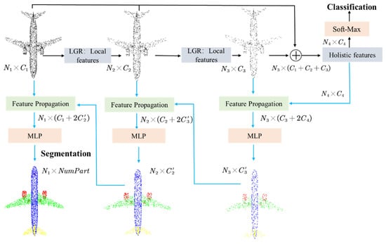
Figure 1.
Local Feature Extraction Network (LFE-Net) architecture for classification and part segmentation. Our network takes the sparse points as input and applies hierarchical architecture for learning features. The key to our network is the Local Geometric Relation (LGR) module, which learns the local features of points and their neighbors as the geometric relation. The classification module concatenates local features from each level to form the holistic features, which are transformed into a 1D descriptor by pooling operation. The part segmentation module propagates the features of sampled points to original points and calculate each point’s scores for N semantic labels.
The two tasks of classification and part segmentation share the same framework of local feature extraction. LFE-Net concatenates all levels’ local features together to fuse all levels’ geometric information and employs algorithms of PointNet to extract holistic features for classification. Then the network transforms holistic features by MLP and pooling operation into different types of probabilities for classification. LFE-Net concatenates the high-dimensional features of low-resolution points and the low-dimensional features of high-resolution points and reduces the dimension of features by a shard MLP, and then the network repeats the same operation from back to front and label each point on the first level for part segmentation.
3.2. Local Geometric Relation (LGR) Module for Local Feature Extraction
This subsection describes the local geometric relation (LGR) module in LFE-Net. Enlightened by PointNet++ [2], we use a ball query with a radius to find neighbors of each centroid. In the first two levels, we set the radius of LGR to 0.1, and 0.3, respectively. Let be the neighbors of centroid . Let be the original geometric feature vector of on the previous layer. We formulate a general convolutional operation for local feature extraction:
where is the output geometric feature obtained by classical CNN and pooling operation, which are expressed by . Next, we introduce 5 different methods about to extract local features.
The first method from PointNet [1] is
which uses a symmetric function to aggregate the information from each point to get the holistic feature but ignores the local geometric information of points and their neighbors.
We can regard the point cloud as image pixels on a regular grid. Similar to AlexNet [22], the second method executes a standard convolution on points and sets the convolution kernel with the same dimension as the output feature vector of the previous layer:
where encodes the weights and denotes the Euclidean inner product.
In addition to considering the features of neighbors , the third method [23] inspired by the above two methods uses the pairwise Euclidean distance between features as the weights of aggregation operation:
and
where is a Gaussian kernel.
The fourth method [3] computes the graph by using nearest neighbors in the feature space and combines neighbor’s feature and neighborhood relation information :
The first method and the second method only focus on the holistic feature extraction and lack the analysis of the local geometric structure of the points. Although the third method and the fourth method augment the geometric connection of the points, these methods use dynamic strategy with large calculation.
We use a normalized method to eliminate the translation of the points by transforming the local points to the local coordinate system. The specific algorithm is to subtract the coordinates of from the coordinates of , in such way that , which remains unchanged during the points translation. This method converts local points to the local coordinate system thus eliminating the translation operation. Then we apply the Singular Value Decomposition (SVD) approach to factor the normalized local points matrix into three new matrices , and , in such way that and let be the singular values of . The singular values indicating the principal orientation of the local points are regarded as geometric relation of local points and concatenated with previous features as the features at each point. We prove the rotation invariance of singular values in Appendix A. Then we use a shared MLP to obtain the joint features of and :
where and . Based on the weight gradient relevant to both and , learns a geometric relation between them. Then we take max pooling operation:
to obtain a 1D feature vector as a generalization of local geometric structure. The pooling operation not only effectively reduces the number of neurons, but also keeps the network invariant to some small local shapes of the points and has a larger receptive field. Additionally, the pooling operation can also be regarded as a bottom-up improvement of the significance to select some key information of the points for analysis, which ensures the network’s invariance to the disorder of the points. Local geometric relation (LGR) module is shown in Figure 2.
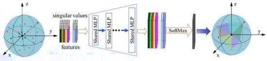
Figure 2.
LGR architecture for local feature extraction. The module takes the sampled points with original geometric features as input. We concatenate the singular values of local points and their features. Then we conduct further channel-raising mapping and pooling operation to generate a 1D vector as a local feature.
3.3. Feature Propagation for Part Segmentation
To complete the task of part segmenting, each point needs to be given a specific label. Although the point clouds without sampling can be direct as the input of each layer of the network and are labeled on the last layer, this method will inevitably increase the calculations and reduce the efficiency of training. Learning from the back-propagation neural network, we take another method to propagate the high-dimensional features of subsampled low-resolution points to original high-resolution points. Then we use an MLP to map concatenated features to new features for all the original points.
The feature propagation algorithm is divided into two steps: First, we use the method of PointNet++ to propagate point features from subsampled points to original points with distance-based interpolation. The second step is to first calculate the distance vectors from the subsampled centroid to the nearest neighbors of the last layer, and then to evenly divide the feature of subsampled centroid into three parts which are respectively multiplied with distance vector coordinate. Finally, we concatenate these two features with the initial features of the high-resolution points to generate new features.
The first step: Traditionally, in order to effectively match image keypoints, it is necessary to generate keypoint descriptors by computing the gradient magnitudes and orientations, which are weighted by distance from neighbors to the keypoint. Our implementation described below is inspired by this idea. For each point in last layer points , we obtain the k-nearest neighbors in subsampled points (in default we use k = 3). As shown in the left part of Figure 3, blue point belongs to and black points , and belong to . We use inverse distance weighted average to interpolate features of at coordinates of the points. We can obtain the sub-feature :
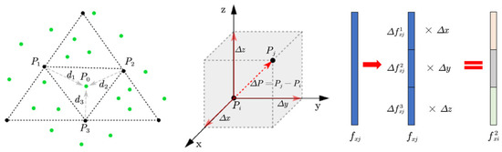
Figure 3.
Illustration of the feature propagation. Left part: Feature interpolation. Middle part: Spatial vector. Right part: Feature segmentation.
The second step: As shown in the middle part of Figure 3, the spatial vector of and is denoted as , which is projected to three axes to get three scalars , and . Then we evenly divide the feature of into three channels , and . As shown in the right part of Figure 3, three scalars of are multiplied to three channels of . Unlike the , we obtain the sub-feature by averaging the feature matrices:
Finally, we use a MLP to obtain the new feature for points:
4. Experiments
In this section, we evaluate LFE-Net by arranging comprehensive experiments of three tasks: classification, part segmentation, and point matching. We also conduct an ablation study to evaluate our network. We apply PyTorch with Python to LFE-Net on one NVIDIA TITAN XP.
4.1. Classification
We evaluate LFE-Net on the ModelNet40 [24] classification task. ModelNet40 contains 12,308 CAD models from 40 categories. We uniformly select 1024 points from each CAD models and take the sampled points only with the (X, Y, Z) coordinates as the input data of the network. Then, we use Adam optimizer with learning rata 0.001, with a batch size of 18 for all the experiments. During training, we augment the data by randomly scaling the points and transforming the points. Meanwhile, we apply dropout technique with 50% in FC layers and randomly drop points during training, which prevent the network from “excessive learning”.
The quantitative comparisons with the state-of-the-art methods are summarized in Table 1. All the experiments are conducted with 1024 points. If we only manipulate the XYZ-points as the input of the LGR module for local feature extraction, the result is only 90.6%. We further test the LGR module with XYZ-Normal-points and the result is improved slightly. If we apply the singular value decomposition (SVD) approach to obtain the local points geometric relation during local feature extraction, LFE-Net will reduce the error rate of PointNet++ by 28.1% and achieve a remarkable result (92.9%) which indicates that our network is superior to others.

Table 1.
Classification results (%) on ModelNet40.
Different resolutions of point clouds may affect the local shape expressions. To verify the reliability of the network, the sampled points of the resolution [24,25,26] respectively input into the trained network. The experimental results are summarized in Figure 4, where the compared networks are PointNet [1], PointNet++ [2], DGCNN [3], PCNN [23], RS-CNN [25]. The rough local structure of low-resolution point clouds increases the difficulty of local feature description. However, our method still achieves significant results compared with other networks.
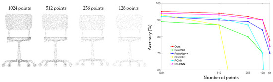
Figure 4.
Left part: Point cloud with random point dropout. Right part: Curve showing test results of using sampled points as the input to compared networks.
4.2. Part Segmentation
We evaluate LFE-Net on the ShapeNetPart [37] segmentation task. ShapeNetPart contains 16,881 shapes from 16 categories and has 50 local parts in total. We uniformly select 2048 points from each training model as input data and each point is labeled to a specific shape. We adopt the same training setting as the classification task.
We use mean Intersection-over-Union (mIoU) as the evaluation scheme, which is averaged across all classes and instances. The quantitative comparisons with the state-of-the-art methods are summarized in Table 2, where LFE-Net achieves the remarkable performance with instance mIoU of 85.7%. LFE-Net is better than the second-best method SpiderCNN 85.3% (0.4% ↑) in instance mIoU. Compared with other XYZ-points networks, LFE-Net achieves new state-of-the-arts over seven categories. As shown in Figure 5, LFE-Net can accurately segment different part shapes out, which demonstrates the robustness of LFE-Net to irregularly distributed points.
Table 2.
Part segmentation results mIoU (%) on non-rotated ShapeNetPart.
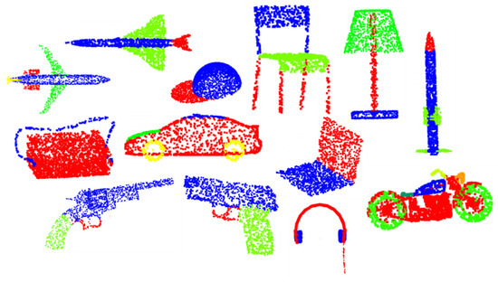
Figure 5.
Part segmentation examples on ShapeNetPart.
It is a challenging task to segment rotated shapes. We compare LFE-Net with the state-of-the-art networks on ShapeNetPart segmentation for rotation-robustness evaluation. We evaluate each network in Table 3 on the shapes with random angles rotation for all three axes (X, Y, Z). Table 3 summarizes the test results in the metric of mIoU. We can find the results of all the networks decreases drastically when the networks take the rotated points as input. Although PointNet++, DGCNN, SpiderCNN, etc. can achieve remarkable results on non-rotated dates, they all fail to effectively analyze the shapes of rotated points and their performance is inferior to ours, and LFE-Net achieves new state-of-the-arts over seven categories on rotated shapes. Figure 6 visualizes that PointNet++ is sensitive to rotation. By contrast, our LFE-Net with local feature learning is invariant to rotation, making it powerful for analyzing the shapes of points.
Table 3.
Part segmentation results mIoU (%) on rotated ShapeNetPart.
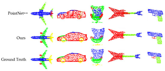
Figure 6.
Visualization of some results on rotated ShapeNetPart. For each set, from top to bottom: PointNet++, ours and ground truth.
4.3. Point Matching
Based on the feature propagation algorithm, we obtain new features with geometric information for each original point and take them as descriptors. Next, we explore the relationships between different part shapes by using our descriptors. As shown in Figure 7, the same part shapes of different point clouds are very similar and the descriptors belonging to the same part shapes are also close to each other in Euclidean space.
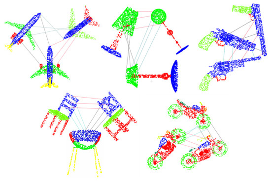
Figure 7.
Descriptor matching performance on the same part shapes of different point clouds.
Three dimensional object recognition is performed by matching each point independently to the database of points from the same shapes. The best candidate match for each point is found by identifying its nearest neighbor, which is defined with minimum Euclidean distance for the invariant descriptor vector. We match the descriptors belonging to the same shape of different point clouds 20% of which are randomly rotated. However, some features from points will not have any correct match in the training database. In order to test the matching accuracy on ShapeNetPart dataset, we set a global threshold on the distance to the closest feature. Table 4 shows the results of our descriptors and the compared methods. The remarkable results indicate that our method is a good option for 3D descriptors.
Table 4.
Descriptor matching results (%).
4.4. Ablation Analysis
We perform a detailed ablation study on the local geometric relation (LGR) module of LFE-Net. The results conducted on ModelNet40 classification are summarized in Table 5. The LGR only with a shared three-layers MLP provides a benchmark which is 80.6%. With the singular values (SVs) of local points as the geometric relation, the accuracy is improved to 82.3%. Then, a great improvement of 2% is because of Batch Normalization (BN). Moreover, the dropout (DP) technique in FC layers leads to a small increase of 1.3%. However, with 2 MLPs and 3 MLPs, the results are improved to 87.4% and 90.1%, respectively. Finally, the best result is 92.9% by adding the voting mechanism.
Table 5.
Ablation study of LGR (%).
There are three symmetric pooling functions in LGR to get a generalization of local geometric structure, including max-pooling (max), average pooling (avg.), and summation (sum). We evaluate the performance of these three functions on ModelNet40 classification and the results are summarized in Table 6. The best strategy for LGR is to use a 3-layers MLP and max pooling, selecting some key information of the points for analysis, as shown in Table 6.
Table 6.
The results (%) of different pooling operations and mapping functions (“-”: unknown).
There are two steps for the feature propagation algorithm, and we evaluate the performance of each step on the ShapeNetPart segmentation. The results are summarized in Table 7. As can be seen, the result of PointNet++ achieving feature propagation only by interpolating feature (IF) values is 85.1% but is improved to 85.2% by adding the method of segmenting feature (SF). Our method with these two steps achieves the best result of 85.7%.
Table 7.
The results (%) of the two steps for feature propagation.
5. Conclusions
In this work, we propose local feature extraction network (LFE-Net) for point cloud analysis. The core to LFE-Net is the LGR module, which extracts local features as the geometric relation of local points. In this way, the local features with the semantic and geometric information are robust to permutation and rigid transformation. To handle the feature propagation issue, we propose two novel steps and combine the two steps to obtain new features for all the original points. These contributions enable us to achieve state-of-the-art performance on classification and part segmentation of 3D point clouds, and the experiments also show that features of all the original points can be used as 3D descriptors in shape analysis and recognition.
Author Contributions
Conceptualization, Z.Z. (Zehao Zhou) and Z.Z. (Zhijiang Zhang); methodology, Z.Z. (Zehao Zhou); software, Z.Z. (Zehao Zhou); validation, Z.Z. (Zehao Zhou), Y.T., and J.C.; formal analysis, Z.Z. (Zehao Zhou); investigation, Z.Z. (Zehao Zhou); resources, Y.T.; data curation, Y.T.; writing—original draft preparation, Z.Z. (Zehao Zhou); writing—review and editing, J.C.; visualization, Z.Z. (Zehao Zhou); supervision, J.C.; project administration, J.C.; All authors have read and agreed to the published version of the manuscript.
Funding
This research was funded by the National Natural Science Foundation of China, grant number 61572307.
Institutional Review Board Statement
Not applicable.
Informed Consent Statement
Not applicable.
Data Availability Statement
Not applicable.
Acknowledgments
This work was supported by the National Natural Science Foundation of China (No. 61572307).
Conflicts of Interest
The authors declare no conflict of interest.
Appendix A
Let local points be a matrix with three nonzero singular values , , . Then there exist a unitary and an unitary such that
where and the singular values are robust to the rotation of local points (See the Figure A1 for illustration).
Proof .
We rotate the local points as , where is a orthogonal matrix. Let
and let
So the main diagonal elements of the matrix are the eigenvalues of . It follows that
In particular, the product of orthogonal matrix and orthogonal matrix does not alter the eigenvectors of . So and have the same singular values, which are robust to the rotation. □

Figure A1.
Illustration of Factoring to .
Figure A1.
Illustration of Factoring to .

References
- Qi, C.R.; Su, H.; Mo, K.; Guibas, L.J. Pointnet: Deep learning on point sets for 3d classification and segmentation. In Proceedings of the IEEE Conference on Computer Vision and Pattern Recognition, Honolulu, HI, USA, 21–26 July 2017; pp. 77–85. [Google Scholar]
- Qi, C.R.; Yi, L.; Su, H.; Guibas, L.J. Pointnet++: Deep hierarchical feature learning on point sets in a metric space. Adv. Neural Inf. Process. Syst. 2017, 30, 5099–5108. [Google Scholar]
- Phan, A.V.; Le Nguyen, M.; Nguyen, Y.L.H.; Bui, L.T. DGCNN: A convolutional neural network over large-scale labeled graphs. Neural Netw. 2018, 108, 533–543. [Google Scholar] [CrossRef]
- Ankerst, M.; Kastenmüller, G.; Kriegel, H.P.; Seidl, T. 3D shape histograms for similarity search and classification in spatial databases. In International Symposium on Spatial Databases; Springer: Berlin/Heidelberg, Germany, 1999; pp. 207–226. [Google Scholar]
- Chaudhuri, S.; Koltun, V. Data-driven suggestions for creativity support in 3D modeling. ACM Trans. Graph. (TOG) 2010, 183, 1–10. [Google Scholar] [CrossRef]
- Saupe, D.; Vranić, D.V. 3D model retrieval with spherical harmonics and moments. In Joint Pattern Recognition Symposium; Springer: Berlin/Heidelberg, Germany, 2001; pp. 392–397. [Google Scholar]
- Osada, R.; Funkhouser, T.; Chazelle, B.; Dobkin, D. Shape distributions. ACM Trans. Graph. (TOG) 2002, 21, 807–832. [Google Scholar] [CrossRef]
- Kazhdan, M.; Funkhouser, T.; Rusinkiewicz, S. Symmetry descriptors and 3D shape matching. In Proceedings of the 2004 Eurographics/ACM SIGGRAPH Symposium on Geometry Processing; Association for Computing Machinery: New York, NY, USA, 2004; pp. 115–123. [Google Scholar]
- Kalogerakis, E.; Hertzmann, A.; Singh, K. Learning 3D Mesh Segmentation and Labeling. ACM Trans. Graph. (TOG) 2010, 29, 1–124. [Google Scholar] [CrossRef]
- Gal, R.; Cohen-Or, D. Salient geometric features for partial shape matching and similarity. ACM Trans. Graph. (TOG) 2006, 25, 130–150. [Google Scholar] [CrossRef]
- Belongie, S.; Malik, J.; Puzicha, J. Shape matching and object recognition using shape contexts. IEEE Trans. Pattern Anal. Mach. Intell. 2002, 24, 509–522. [Google Scholar] [CrossRef]
- Kokkinos, I.; Bronstein, M.M.; Litman, R.; Bronstein, A.M. Intrinsic shape context descriptors for deformable shapes. In Proceedings of the 2012 IEEE Conference on Computer Vision and Pattern Recognition, Providence, RI, USA, 16–21 June 2012; pp. 159–166. [Google Scholar]
- Riegler, G.; Osman Ulusoy, A.; Geiger, A. Octnet: Learning deep 3d representations at high resolutions. In Proceedings of the IEEE Conference on Computer Vision and Pattern Recognition, Honolulu, HI, USA, 21–26 July 2017; pp. 6620–6629. [Google Scholar]
- Maturana, D.; Scherer, S. Voxnet: A 3d convolutional neural network for real-time object recognition. In Proceedings of the 2015 IEEE/RSJ International Conference on Intelligent Robots and Systems (IROS), Hamburg, Germany, 28 September–2 October 2015; pp. 922–928. [Google Scholar]
- Ono, Y.; Trulls, E.; Fua, P.; Yi, K.M. LF-Net: Learning local features from images. arXiv 2018, arXiv:1805.09662. [Google Scholar]
- Su, H.; Maji, S.; Kalogerakis, E.; Learned-Miller, E. Multi-view Convolutional Neural Networks for 3D Shape Recognition. In Proceedings of the IEEE International Conference on Computer Vision, Santiago, Chile, 7–13 December 2015; pp. 945–953. [Google Scholar]
- Chen, X.; Ma, H.; Wan, J.; Li, B.; Xia, T. Multi-view 3d object detection network for autonomous driving. In Proceedings of the IEEE Conference on Computer Vision and Pattern Recognition, Honolulu, HI, USA, 21–26 July 2017; pp. 6526–6534. [Google Scholar]
- Kalogerakis, E.; Averkiou, M.; Maji, S.; Chaudhuri, S. 3D shape segmentation with projective convolutional networks. In Proceedings of the IEEE Conference on Computer Vision and Pattern Recognition, Honolulu, HI, USA, 21–26 July 2017; pp. 6630–6639. [Google Scholar]
- Qi, X.; Liao, R.; Jia, J.; Fidler, S.; Urtasun, R. 3d graph neural networks for rgbd semantic segmentation. In Proceedings of the IEEE International Conference on Computer Vision, Venice, Italy, 22–29 October 2017; pp. 5209–5218. [Google Scholar]
- Hu, Q.; Yang, B.; Xie, L.; Rosa, S.; Guo, Y.; Wang, Z. RandLA-Net: Efficient semantic segmentation of large-scale point clouds. In Proceedings of the IEEE/CVF Conference on Computer Vision and Pattern Recognition, Seattle, WA, USA, 13–19 June 2020; pp. 11105–11114. [Google Scholar]
- Han, W.; Wen, C.; Wang, C.; Li, X.; Li, Q. Point2Node: Correlation learning of dynamic-node for point cloud feature modeling. In Proceedings of the AAAI Conference on Artificial Intelligence, New York, NY, USA, 7–12 February 2020; Volume 34, pp. 10925–10932. [Google Scholar]
- Krizhevsky, A.; Sutskever, I.; Hinton, G.E. Imagenet classification with deep convolutional neural networks. Adv. Neural Inf. Process. Syst. 2012, 25, 1097–1105. [Google Scholar] [CrossRef]
- Atzmon, M.; Maron, H.; Lipman, Y. Point convolutional neural networks by extension operators. arXiv 2018, arXiv:1803.10091. [Google Scholar] [CrossRef]
- Wu, Z.; Song, S.; Khosla, A.; Yu, F.; Zhang, L.; Tang, X.; Xiao, J. 3D Shapenets: A Deep Representation for Volumetric Shapes. In Proceedings of the IEEE International Conference on Computer Vision and Pattern Recognition (CVPR), Boston, MA, USA, 7–12 June 2015; pp. 1912–1920. [Google Scholar]
- Liu, Y.; Fan, B.; Xiang, S.; Xiang, S.; Pan, C. Relation-shape convolutional neural network for point cloud analysis. In Proceedings of the IEEE Conference on Computer Vision and Pattern Recognition, Long Beach, CA, USA, 15–20 June 2019; pp. 8895–8904. [Google Scholar]
- Hua, B.S.; Tran, M.K.; Yeung, S.K. Pointwise convolutional neural networks. In Proceedings of the IEEE Conference on Computer Vision and Pattern Recognition, Salt Lake City, UT, USA, 18–23 June 2018; pp. 984–993. [Google Scholar]
- Simonovsky, M.; Komodakis, N. Dynamic edge-conditioned filters in convolutional neural networks on graphs. In Proceedings of the IEEE Conference on Computer Vision and Pattern Recognition, Honolulu, HI, USA, 21–26 July 2017; pp. 29–38. [Google Scholar]
- Xie, S.; Liu, S.; Chen, Z.; Tu, Z. Attentional ShapeContextNet for Point Cloud Recognition. In Proceedings of the IEEE Conference on Computer Vision and Pattern Recognition, Salt Lake City, UT, USA, 18–23 June 2018; pp. 4606–4615. [Google Scholar]
- Gadelha, M.; Wang, R.; Maji, S. Multiresolution tree networks for 3d point cloud processing. In Proceedings of the European Conference on Computer Vision (ECCV), Munich, Germany, 8–14 September 2018; pp. 103–118. [Google Scholar]
- Li, J.; Chen, B.M.; Hee Lee, G. So-net: Self-organizing network for point cloud analysis. In Proceedings of the IEEE Conference on Computer Vision and Pattern Recognition, Salt Lake City, UT, USA, 18–23 June 2018; pp. 9397–9406. [Google Scholar]
- Groh, F.; Wieschollek, P.; Lensch, H. Flex-convolution (million-scale point-cloud learning beyond grid-worlds). arXiv 2018, arXiv:1803.07289. [Google Scholar]
- Wang, C.; Samari, B.; Siddiqi, K. Local spectral graph convolution for point set feature learning. In Proceedings of the European Conference on Computer Vision (ECCV), Munich, Germany, 8–14 September 2018; pp. 52–66. [Google Scholar]
- Shen, Y.; Feng, C.; Yang, Y.; Tian, D. Mining point cloud local structures by kernel correlation and graph pooling. In Proceedings of the IEEE Conference on Computer Vision and Pattern Recognition, Salt Lake City, UT, USA, 18–23 June 2018; pp. 4548–4557. [Google Scholar]
- Klokov, R.; Lempitsky, V. Escape from cells: Deep kd-networks for the recognition of 3d point cloud models. In Proceedings of the IEEE International Conference on Computer Vision, Honolulu, HI, USA, 21–26 July 2017; pp. 863–872. [Google Scholar]
- Yang, J.; Zhang, Q.; Ni, B.; Li, L.; Liu, J. Modeling point clouds with self-attention and gumbel subset sampling. In Proceedings of the IEEE Conference on Computer Vision and Pattern Recognition, Long Beach, CA, USA, 15–20 June 2019; pp. 3318–3327. [Google Scholar]
- Xu, Y.; Fan, T.; Xu, M.; Zeng, L.; Qiao, Y. Spidercnn: Deep learning on point sets with parameterized convolutional filters. In Proceedings of the European Conference on Computer Vision (ECCV), Munich, Germany, 8–14 September 2018; pp. 87–102. [Google Scholar]
- Yi, L.; Kim, V.G.; Ceylan, D.; Shen, I.; Yan, M.; Su, H.; Lu, A.; Huang, Q.; Sheffer, A.; Guibas, L. A Scalable Active Framework for Region Annotation in 3D Shape Collections. TOG 2016, 35, 210. [Google Scholar] [CrossRef]
- Huang, Q.; Wang, W.; Neumann, U. Recurrent slice networks for 3d segmentation of point clouds. In Proceedings of the IEEE Conference on Computer Vision and Pattern Recognition, Salt Lake City, UT, USA, 18–23 June 2018; pp. 2626–2635. [Google Scholar]
- Su, H.; Jampani, V.; Sun, D.; Maji, S.; Kalogerakis, E.; Yang, M.-H.; Kautz, J. SPLATNet: Sparse lattice networks for point cloud processing. In Proceedings of the IEEE Conference on Computer Vision and Pattern Recognition, Salt Lake City, UT, USA, 18–23 June 2018; pp. 2530–2539. [Google Scholar]
- Tombari, F.; Salti, S.; Di Stefano, L. Unique signatures of histograms for local surface description. In Proceedings of the European Conference on Computer Vision, Grete, Greece, 5–11 September 2010; pp. 356–369. [Google Scholar]


Publisher’s Note: MDPI stays neutral with regard to jurisdictional claims in published maps and institutional affiliations. |
© 2021 by the authors. Licensee MDPI, Basel, Switzerland. This article is an open access article distributed under the terms and conditions of the Creative Commons Attribution (CC BY) license (http://creativecommons.org/licenses/by/4.0/).