Article

Item Response Theory Models for the Fuzzy TOPSIS in the Analysis of Survey Data

by
Bartłomiej Jefmański
1,* and
Adam Sagan
2,3
1
Department of Econometrics and Computer Science, Wroclaw University of Economics and Business, 53–345 Wrocław, Poland
2
Department of Market Analysis and Marketing Research, Cracow University of Economics, 31–510 Cracow, Poland
3
Institute of Sociology, Jagiellonian University, 31–044 Cracow, Poland
*
Author to whom correspondence should be addressed.
Symmetry 2021, 13(2), 223; https://doi.org/10.3390/sym13020223
Submission received: 29 December 2020 / Revised: 20 January 2021 / Accepted: 26 January 2021 / Published: 29 January 2021

Abstract

:
The fuzzy TOPSIS (The Technique for Order of Preference by Similarity to Ideal Solution) is an attractive tool for measuring complex phenomena based on uncertain data. The original version of the method assumes that the object assessments in terms of the adopted criteria are expressed as triangular fuzzy numbers. One of the crucial stages of the fuzzy TOPSIS is selecting the fuzzy conversion scale, which is used to evaluate objects in terms of the adopted criteria. The choice of a fuzzy conversion scale may influence the results of the fuzzy TOPSIS. There is no uniform approach in constructing and selecting the fuzzy conversion scale for the fuzzy TOPSIS. The choice is subjective and made by researchers. Therefore, the aim of the article is to present a new, objective approach to the construction of fuzzy conversion scales based on Item Response Theory (IRT) models. The following models were used in the construction of fuzzy conversion scales: Polychoric Correlation Model (PM), Polytomous Rasch Model (PRM), Rating Scale Model (RSM), Partial Credit Model (PCM), Generalized Partial Credit Model (GPCM), Graded Response Model (GRM), Nominal Response Model (NRM). The usefulness of the proposed approach is presented on the example of the analysis of a survey’s results on measuring the quality of professional life of inhabitants of selected communes in Poland. The obtained results indicate that the choice of the fuzzy conversion scale has a large impact on the closeness coefficient values. A large difference was also observed in the spreads of triangular fuzzy numbers between scales based on IRT models and those used in the literature on the subject. The use of the fuzzy TOPSIS with fuzzy conversion scales built based on PRM, RSM, PCM, GPCM, and GRM models gives results with a greater range of variability than in the case of fuzzy conversion scales used in empirical research.

1. Introduction

In socio-economic research, the assessment of objects (countries, cities, and organizations) in terms of complex phenomena (sustainable development, quality of life, and quality of services) is carried out using questionnaire studies and ordinal measurement scales (most often the Likert scales). As complex phenomena are subject to assessment, an unambiguous assessment of objects is difficult. The solution may be using multi-criteria decision-making methods (MCDM) that allow taking into account the influence of many partial criteria (sub-criteria) on complex phenomena. In the analysis of complex socio-economic phenomena using MCDM methods, the Technique for Order of Preference by Similarity to Ideal Solution (TOPSIS) method is particularly popular [1].
The TOPSIS method has gone through many modifications [2,3,4,5]. One of the research directions on the TOPSIS method as part of the methodological trend is an attempt to take into account the uncertainty of measurement results using the fuzzy set theory. The first proposal in this area was the fuzzy TOPSIS method [6], whose criteria values can be expressed as fuzzy numbers. It is a particularly useful modification for the analysis of complex socio-economic phenomena as it enables the measurement of these phenomena using fuzzy scales or fuzzy conversion scales. These are scales in which individual categories are most often expressed in triangular or trapezoidal fuzzy numbers. The difference between these scales is that the respondents set the parameters of fuzzy numbers themselves in the first case. In contrast, in the second case, a classic measurement is made using ordinal scales, and then the measurement results are converted to the form of fuzzy numbers. The second approach is more prevalent in the literature.
The fuzzy conversion scales used with the fuzzy TOPSIS most often have five points (categories) represented by five triangular fuzzy numbers. The 6-point and 7-point scales are used less frequently (see, e.g., [7,8]). The values of the parameters of triangular fuzzy numbers differ from study to study. There are also differences in the spread of triangular fuzzy numbers. In the studies [9,10], the triangular fuzzy numbers’ lower and upper limit values are in the interval <0; 1>. In both studies, the spreads of fuzzy numbers for extreme categories differ from the others. Triangular fuzzy numbers assigned to the remaining categories are symmetric and have the same spread. In the study [10], the spreads of adjacent fuzzy numbers overlap to a greater extent. A similar fuzzy conversion scale was used in the study [11]. The difference concerns the middle category, where the triangular fuzzy number has the largest spread compared to the other triangular fuzzy numbers. Another proposal for a fuzzy conversion scale is presented in [12]. The lower and upper limit values of triangular fuzzy numbers belong to the interval <0.1; 0.9>. Triangular fuzzy numbers are symmetric except in the extreme categories. However, the scale is distinguished because the ranges of triangular fuzzy numbers do not overlap.
Fuzzy conversion scales are also used in the research, where the lower and upper limit values of the triangular fuzzy numbers belong to the interval <0; 5>. An example may be the study [13]. In the scale used, the extreme category expressing the highest score has an asymmetric triangular fuzzy number. The remaining triangular fuzzy numbers are symmetric and have the same spreads. Spreads of adjacent triangular fuzzy numbers overlap.
A popular approach in constructing fuzzy conversion scales for the fuzzy TOPSIS is to determine the parameters of triangular fuzzy numbers based on a value in the interval <0; 10>. An example may be the scales proposed in [14,15]. The scales are characterized by a large spread of the triangular fuzzy number assigned to the middle category. Triangular fuzzy numbers assigned to the remaining categories are asymmetric. The smallest spreads have fuzzy numbers assigned to extreme categories. A characteristic feature of these scales is that the ranges of triangular fuzzy numbers do not overlap (except for the extreme categories).
Lower and upper limit values of the triangular fuzzy numbers from the interval <0; 10> were also used in [16]. However, on this scale, the spreads of adjacent fuzzy numbers overlap. The spreads of all triangular fuzzy numbers are very close.
Another fuzzy conversion scale was used in [17]. The parameters of triangular fuzzy numbers were established on the basis of the values in the interval <0; 9>. The scale is characterized by the same but large range of fuzzy numbers for the middle categories. Nădăban et al. [2] proposed a scale similar to [17]. The difference concerns the fourth and five categories (positive categories) where the shapes and spreads of the fuzzy number domains are different.
The fuzzy conversion scales presented above do not exhaust all possible combinations of assigning triangular fuzzy numbers to categories of ordinal measurement scales. However, it can be noticed that the extreme categories often have the smallest ranges of triangular fuzzy numbers, which suggests that they are relative “precisely” interpreted, perceived by experts and researchers. It is common practice to establish equal ranges of the triangular fuzzy number for the categories representing the middle of the measurement scale. It is difficult to indicate the dominant range of values in determining the lower and upper limit values of the triangular fuzzy numbers. There is also no rule about the location of the triangular fuzzy numbers on the measurement scale. Ranges of triangular fuzzy numbers may overlap more or less. Fuzzy conversion scales are also used where the ranges of triangular fuzzy numbers do not overlap.
Regardless of the area of application of the fuzzy TOPSIS in connection with fuzzy conversion scales, the method of determining the parameters of fuzzy numbers assigned to categories of the ordinal measurement scales is debatable. It usually subjectively takes place because it is most often determined by researchers or experts (see for example [7,8,9,10,11,12,13,14,15,16,17]). Therefore, the article presents a new proposal of the method for determining the parameters of fuzzy conversion scales for the fuzzy TOPSIS method based on the respondents’ opinions who assess the partial criteria. The proposed method uses the achievements of the Item Response Theory (IRT). We developed several simulations for determining the parameters of fuzzy conversion scales based on prominent IRT models, namely, Polytomous Rasch Model, Rating Scale Model, Partial Credit Model, Generalized Partial Credit Model, Graded Response Model, and Nominal Response Model. Model-based conversions were compared to conversions based on a model-free polychoric correlation approach and simple ordinal rating (Likert) scale. Model-based conversions enable us to estimate thresholds given continuous latent variable as an IRT model outcome. Based on thresholds estimated for selected IRT models, a method of determining the parameters of triangular fuzzy numbers for fuzzy conversion scales was proposed. As the method of estimating the thresholds differs within IRT models, the thresholds for five IRT models were estimated and compared.
The manuscript is organized as follows. In the Section 2, the fuzzy TOPSIS is presented. Selected IRT models are characterized in Section 3. Then, a method of constructing fuzzy conversion scales based on threshold values obtained using IRT models was proposed. Section 4 presents the usefulness of the proposed approach based on an empirical example concerning assessing the quality of professional life of residents of selected communes in Poland. In Section 5, the obtained results were compared with other fuzzy conversion scales used in conjunction with the fuzzy TOPSIS. Finally, the conclusions of the paper are presented.

2. Fuzzy TOPSIS Method

Classical MCDM methods assume that criteria and weights are expressed in crisp values. However, in many real situations, the assessments of criteria are often expressed qualitatively or using linguistic expressions [18]. In such a case, the theory of fuzzy sets proposed by Zadeh [19] applies. The fuzzy set theory, combined with the appropriate fuzzy modifications of the MCDM methods, allows analyzing imprecise and fuzzy information. One of such methods is the fuzzy TOPSIS proposed by Chen [6]. The method assumes that the assessments of criteria and their weights can be expressed as triangular fuzzy numbers.
Definition 1.
[20]. If X is a collection of objects denoted generically by x then a fuzzy set A ˜ in X is a set of ordered pairs:
A ˜ = { ( x , μ A ˜ ( x ) ) | x X }
where μ A ˜ is the membership function that maps X to the membership space M and μ A ˜ ( x ) is the grade of membership (also degree of compatibility or degree of truth) of x in A ˜ .
Definition 2.
[6]. A fuzzy number is a fuzzy subset in the universe of discourse X that is both convex and normal.
Definition 3.
[6]. A triangular fuzzy number A can be defined by a triplet ( a , b , c ) . The membership function μ A ( x ) is defined as
μ A ( x ) = { 0 , x < a x a b a , a x b x c b c , b x c 0 , x > c .
Definition 4.
[6]. Let A 1 = ( a 1 , b 1 , c 1 ) and A 2 = ( a 2 , b 2 , c 2 ) be two triangular fuzzy numbers, then the vertex method is defined to calculate the distance between them as
d ( A 1 , A 2 ) = 1 3 [ ( a 1 a 2 ) 2 + ( b 1 b 2 ) 2 + ( c 1 c 2 ) 2 ] .
Let us assume that a research trial has K respondents, then the importance of the criteria and the assessment of alternatives (objects) with respect to each criterion can be calculated as
x ˜ i j = 1 K [ x ˜ i j 1 + x ˜ i j 2 + + x ˜ i j K ]
w ˜ j = 1 K [ w ˜ j 1 + w ˜ j 2 + + w ˜ j K ]
where x ˜ i j K = ( a i j K , b i j K , c i j K ) and w ˜ j K = ( a ( w ) i j K , b ( w ) i j K , c ( w ) i j K ) are the assessment and importance weight of the K -th respondent in the form of triangular fuzzy numbers. A fuzzy multi-criteria group decision making problem can be expressed in fuzzy decision matrix as
D ˜ = [ x ˜ 11 x ˜ 12 x ˜ 1 n x ˜ 21 x ˜ 22 x ˜ 2 n x ˜ m 1 x ˜ m 2 x ˜ m n ] ( i = 1 , 2 , , m ) ( j = 1 , 2 , , n )
W ˜ = [ w ˜ 1 , w ˜ 2 , , w ˜ n ]
where x ˜ i j = ( a i j , b i j , c i j ) , w ˜ j = ( a ( w ) j , b ( w ) j , c ( w ) j ) .
Ranking of objects with the above-outlined assumptions is possible among others through the application of the fuzzy TOPSIS.
Application of fuzzy TOPSIS method requires the accomplishment of the following steps [6]:
Step 1. Construction of normalized fuzzy decision matrix R ˜ = [ r ˜ i j ] m × n
R ˜ = [ r ˜ 11 r ˜ 12 r ˜ 1 n r ˜ 21 r ˜ 22 r ˜ 2 n r ˜ m 1 r ˜ m 2 r ˜ m n ] .
This stage requires an indication of benefit ( B ) and cost criteria ( C ). The normalization formulas for benefit and cost criteria have the form, respectively:
r ˜ i j = ( a i j c j + , b i j c j + , c i j c j + ) j B
r ˜ i j = ( a j c i j , a j b i j , a j a i j ) j C
where c j + = max c i j if j B and a j = min a i j if j C .
Step 2. Construction of weighted normalized fuzzy decision matrix V ˜ = [ v i j ] m × n
V ˜ = [ v ˜ 11 v ˜ 12 v ˜ 1 n v ˜ 21 v ˜ 22 v ˜ 2 n v ˜ m 1 v ˜ m 2 v ˜ m n ]
where v ˜ i j = r ˜ i j w ˜ j .
Step 3. Determining fuzzy positive ideal solution A ˜ + and fuzzy negative ideal solution A ˜ , respectively:
A ˜ + = ( v ˜ 1 + , v ˜ 2 + , , v ˜ n + )
A ˜ = ( v ˜ 1 , v ˜ 2 , , v ˜ n )
where v ˜ j + = ( 1 , 1 , 1 ) and v ˜ j = ( 0 , 0 , 0 ) .
Step 4. Calculation of the distance of each object from fuzzy positive ideal solution A ˜ + and fuzzy negative ideal solution A ˜ , respectively:
d i + = j = 1 n d ( v ˜ i j , v ˜ j + )
d i = j = 1 n d ( v ˜ i j , v ˜ j )
where d is the distance between two triangular fuzzy numbers (3).
Step 5. Calculation of the closeness coefficient C C i for each object
C C i = d i d i + + d i .
C C i values are normalized in an interval < 0 ; 1 > . The smaller the distance of an object is from a positive ideal solution, and the bigger from a negative ideal solution, the closer the value of a closeness coefficient is to 1.
Step 6. Establishing the objects ranking. The best object owns the biggest value of a closeness coefficient (16).

3. Materials and Methods

3.1. Ordinal Items and Threshold Values

The ordered categories on the hypothesized continuum are continuous. They are separated on the continuum by successive points termed thresholds. This is analogous to mapping a location of an object on a line partitioned into equal units to obtain a physical measurement. Because in ordinal or interval data there is no fixed origin, there is also no endpoint on the latent continuum. The simplest way to operationalize the threshold for ordinal data point is the concept of latent response variable (LRV). LRV is regarded as a better approximation of imperfect ordinal scales and are based on normal-ogive probit transformation of original data. The correlations estimated on the basis of transformed ordinal data are called polychoric correlations and are regarded as non-attenuated correlations (in comparison to Pearson product-moment correlations) between ordinal items.
Two methods are used in calculation of polychoric correlation. The first method, the joint maximum likelihood approach, estimates all model parameters—correlation and the thresholds—at the same time. The second method, two-step ML estimation, first estimates the thresholds from the one-way marginal frequencies, then estimates polychoric correlation, conditional on these thresholds, via maximum likelihood [21]. The number of thresholds is k-1 for k-category of ordinal Likert scale. Model for LRV linking five ordinal categories to corresponding latent response variable is given as
y = { 1   if   y τ 1 2   if   τ 1 < y τ 2 3   if   τ 2 < y τ 3 4   if   τ 3 < y τ 4 5   if   y τ 4
where y * is latent response variable, and τ is a threshold.
Ordinal items and the threshold values are key concepts in psychometric measurement models. Two basic types of measurement models can be distinguished: 1/Classical Test Theory (CTT) and 2/Item Response Theory (IRT). CTT is based on confirmatory factor analysis (as a latent variable model) of covariance or Pearson product-moment correlation matrix of indicators, that represents the set of highly intercorrelated items measured on interval scale. In case of ordinal scales the Pearson correlations are replaced by tetrachoric (for binary data) or polychoric correlations (for ordinal data) that are estimated on the basis of k-1 thresholds for k categories. Additionally, the set of items are characterized by the equality of items discrimination (equal factor loadings) and equality of items intercepts [22,23].
IRT models represents modern approach to psychometric measurement, that is related to conditional probability of response to specific binary item or specific category of ordinal item, given respondent ability (his/her position on latent trait continuum). The probability is described by logistic or normal ogive characteristic curves for each item. Additionally, the set of items can be characterized by non-equal item discrimination parameters and non-equal item difficulty parameters that are related to the threshold values [22,24].
In IRT models, thresholds are defined as boundaries between adjacent scores and serve as successive “steps” in an item response process. The concept of threshold is key element in polytomous Likert-type scaling (like 5—point ordinal scale) where two types of probabilities can be distinguished: (a) probability of passing a category boundary threshold (item step), and (b) probability of responding in the next category of scale. So, thresholds are also sometimes referred to as category boundaries, which separate the ordered response categories. The definition and modelling of category boundaries depends on the type of polytomous IRT model. In the family of graded response model (GRM) the cumulative model is used, whereas in Rasch-type model (Polytomous Rasch Model (PRM), Partial Credit Model (PCM), and Rating Scale Model (RSM)), the adjacent category model is preferred [24]. Therefore, the concept of threshold and interpretation of location parameter depends on applied model.

3.2. Polytomous Rasch Model

The polytomous Rasch model is generalization of dichotomous Rasch model for binary data. When the model has the same format across all items and has the same sized categories is referred to sometimes as the Partial Credit Model or Rating Scale Model with constrained slopes parameters as 1. Model is given as [25]:
P i k ( θ ) = exp k = 1 n ( θ δ i k ) 1 + k = 1 m i exp k = 1 n ( θ δ i k )
where δ i k is the item difficulty (location) parameter for k-th category of i-th item. The threshold corresponds with the location on θ latent continuum at which it is equal probability of respondent’s classification into adjacent categories, and to obtain one of two successive scale scores (1 or 2, 2 or 3, etc.).
The PRM has two properties: first, combining adjacent categories by summing the probabilities of responses in the categories, and in the related sense of summing their frequencies to form a single category, can only be done under very restricted circumstances. Second, the thresholds define the boundaries of the successive categories may take on values that are not in their natural order.
Polytomous Rasch model is the most constrained model presented in the paper and most popular IRT model concentrated on location (difficulty) parameters. For this model, more detailed information is provided.
Item Characteristic Curves (ICC) show logistic (for extreme categories) and probit (for middle categories) functions, based on conditional probabilities of responding to specific item category (1–5), given position on latent trait continuum ( θ score). The number of curves equals the number of item categories. The higher Ability score, the lower probability of choosing weakest category (1) and the higher probability of choosing the strongest category (5). The probabilities of middle categories (2, 3, 4) are described by probit curves, where probability is rising to specific Ability score, and falling beyond this point. The intersection of adjacent categories (1–2, 2–3, 3–4) indicates the equality of conditional probability responding to adjacent categories. The intersection points are equal to threshold values of Ability score. Item Operation Characteristic Curves (on right panels) represent the logit models of upper boundary threshold probabilities. The number of curves equals the number of thresholds. The inflection point on each curve indicates the equal probability (0.5) of choosing one of adjacent category.

3.3. Rating Scale Model

RSM model is a version of PRM:
P i k ( θ ) = exp k = 0 n ( θ ( δ i + τ k ) ) i = 0 m 1 exp k = 0 n ( θ ( δ i + τ k ) )
where δ i is the item difficulty (location) parameter, τ k is the common category boundary (threshold) parameter for all the items using a particular rating scale and θ is a latent trait variable. Model assumes that all items are equally discriminating (constant discrimination parameter = 1). As a consequence distances between thresholds are the same across items, with the only difference among the item parameters being the location of the item determined by the mean of the thresholds. In the result, thresholds for the categories differ in RSM from each other by an amount that is constant across items.

3.4. Partial Credit Model and Generalized Partial Credit Model

The partial credit model (PCM) developed by G. N. Masters belongs to the Rasch family of item response models [26]. E. Muraki’s extension of Generalized Partial Credit Model (GPCM), includes additional discrimination parameter that removes GPCM from the family of Rasch models [27]. In partial credit model each probability of choosing given category (k) over adjacent (k-1) category of Likert scale is explained by dichotomous response model. In PCM the conditional probability of choosing given category is given as
P i k ( θ ) = exp j = 0 k ( θ δ i k ) i = 0 m 1 exp j = 0 i ( θ δ i k )
where δ i k is the difficulty (location) parameter for category boundary (threshold) parameter k of item i and θ is a latent trait variable. Item-category threshold parameter can be given as an intersection point of P i k ( θ ) and P i , k + 1 ( θ ) .
The GPCM is two-parameter PCM model:
P i k ( θ ) = exp k = 0 n 1.7 a i ( θ δ i + d k ) i = 0 m 1 exp j = 0 i ( θ δ i + d k )
where a i is a common slope (discrimination) parameter, δ i is an item difficulty (location) parameter and d k is the category boundary (threshold) parameter. The d k define how far from an item location a threshold is.

3.5. Graded Response Model

GRM is a logistic model given by the equation:
P i k ( θ ) = exp [ a i ( θ δ i k ) ] 1 + exp [ a i ( θ δ i k ) ] exp [ a i ( θ δ i k + 1 ) ] 1 + exp [ a i ( θ δ i k + 1 ) ]
where a i is the item discrimination parameter, and δ i k is the difficulty (location) parameter for category boundary (threshold) parameter k of item i.

3.6. Nominal Response Model

NRM is an IRT model for unordered multiple choice questions or “yes”, “no”, “don’t know” type of questions. No implicit ordering of scale categories is required. The model is given by the equation:
P i k ( θ ) = exp ( a k θ + δ k ) i exp ( a i θ + δ i )
where a k is the category slope parameter and δ k is the category intercept parameter (attractiveness of the k-th category, that helps to interpret the ordering of the categories). Additionally, k = 1 m i a i k = 0 and k = 1 m i δ i k = 0 .

3.7. Method of Constructing Fuzzy Conversion Scales for the Fuzzy TOPSIS Method

The proposed method assumes the conversion of the measurement results in triangular fuzzy numbers because they are most often used in the fuzzy TOPSIS. The conversion method was divided into four stages, as shown in Figure 1.
Stage 1. Evaluation of objects in terms of partial criteria using ordinal measurement scales.
Let us assume that a set of objects is assessed in terms of a complex phenomenon characterized by partial criteria. Assessment of objects in terms of partial criteria are obtained during a survey using a questionnaire. Each of the objects is assessed in terms of partial criteria by the respondents using the same ordinal measurement scale with the following categories: 1—very low (VL), 2—low (L), 3—medium (M), 4—high (H), 5—very high (VH).
Stage 2. Calculation of the thresholds for each of the criteria.
The respondents’ assessments obtained in the first stage should be used to determine the thresholds. Thresholds are estimated separately for each of the partial criteria. The choice of the IRT model based on which the thresholds will be estimated up to the researcher considers the assumptions and properties of individual models.
Stage 3. Conversion of the categories on the ordinal measurement scale to the triangular fuzzy numbers with the use of thresholds.
Conversion of the categories on the ordinal measurement scale to triangular fuzzy numbers uses the threshold values estimated in step 2. The method of determining the parameters of fuzzy numbers differs depending on the category’s position on the ordinal measurement scale. The formulas for determining the parameters of triangular fuzzy numbers for each category are presented in Table 1.
The parameters of triangular fuzzy numbers should be estimated separately for each of the partial criteria. It is easy to notice that some parameters of the triangular fuzzy numbers that replace the extreme categories are arbitrarily set at the level of −4 and 4. This procedure allowed for both the left and right limitation of the measurement scale. The adopted values result from the fact that in IRT models, the hidden variable continuum is often limited to the range <−4; 4>. It should also be emphasized that the parameters of triangular fuzzy numbers can be scaled by a selected constant value set arbitrarily by the researcher.
Stage 4. Conversion of the measurement results into triangular fuzzy numbers.
Each assessment of the object in terms of the respondents’ selected partial criterion is transformed into a triangular fuzzy number. This procedure should be repeated for the remaining criteria, remembering that triangular fuzzy numbers’ parameters may differ even though they replace the same category on the ordinal scale. Given the assessments in the form of triangular fuzzy numbers, calculate the mean score of the object for each criterion according to arithmetic rules for triangular fuzzy numbers. The averaged scores will also be in the form of triangular fuzzy numbers. The criteria values for each of the objects calculated in this way can be used in the fuzzy TOPSIS method.
The research process using the proposed approach to the construction of fuzzy conversion scales and the fuzzy TOPSIS method was summarized in the form of a flow chart (Figure 2).

4. Empirical Example

The method of constructing fuzzy conversion scales using IRT models for the fuzzy TOPSIS is presented on the example of assessing the quality of professional life. The quality of professional life was one of a larger survey on the quality of life of inhabitants of a selected county in Poland. The study was conducted in 2017 in the form of individual interviews using a questionnaire. The selection of respondents for the study was proportional strata sampling. The sample size was determined based on statistical data published by Statistics Poland. The planned sample size was 1.047 respondents. One thousand fifty-four correctly completed questionnaires were received. The maximum sampling error was 0.03. The size of error indicates that the research results can be considered highly precise and representative for the analyzed county. The assumed and obtained sample distribution by place of residence is presented in Table 2.
The aim of the study was to establish a ranking of five communes in terms of the quality of professional life of their inhabitants. The quality of professional life as a complex phenomenon has been characterized in terms of 12 criteria: C1—job security, C2—salary, C3—promotion opportunities, C4—development opportunities, C5—chances of finding a new comparable or better job, C6—relations with colleagues, C7—relations with superiors, C8—understanding of the employer, C9—justice of the superior, C10—communication in the workplace, C11—material working conditions, C12—the flexibility of working time. In the evaluation of communes, in terms of the adopted criteria, an ordinal measurement scale was used with the following categories: 1—very low (VL), 2—low (L), 3—medium (M), 4—high (H), 5—very high (VH). The research did not consider answers such as “don’t know”, “I have no opinion”; therefore, the final analysis included the opinions of 939 respondents. According to the methodology presented in Section 3.7, the measurement results using the ordinal measurement scale are used to determine the thresholds. The thresholds were established for each of the criteria. All IRT models described in Section 3 were used to estimate thresholds, which allowed for a comparative analysis of the obtained results. The thresholds for the models are shown in Table 3, Table 4, Table 5, Table 6, Table 7, Table 8, Table 9, Table 10, Table 11, Table 12, Table 13, Table 14, Table 15 and Table 16.
Thresholds can be also graphically represented as characteristic curves. An example of such curves for each item and operation characteristic curves obtained based on the PRM is presented in Figure 3, Figure 4, Figure 5, Figure 6, Figure 7, Figure 8, Figure 9, Figure 10, Figure 11, Figure 12, Figure 13 and Figure 14.
Based on each item’s thresholds, the parameters of triangular fuzzy numbers corresponding to the five points of the ordinal measurement scale were determined (in line with stage 3 of the proposed methodology). The values of the estimated parameters are presented in Table 17, Table 18, Table 19, Table 20, Table 21, Table 22, Table 23, Table 24, Table 25, Table 26, Table 27, Table 28, Table 29 and Table 30.
The obtained triangular fuzzy numbers can also be presented graphically (as in Figure 1). Due to the large number of fuzzy numbers obtained, only the fuzzy numbers estimated using the PRM are presented as an example (Figure 15).
The ordinal measurement scale with five categories used to assess five communes against 12 criteria is replaced with the corresponding fuzzy conversion scales. It means that triangular fuzzy numbers now represent the categories on the ordinal scale. Suppose for each commune we average the respondents’ assessment for each criterion (according to the rules of arithmetic for triangular fuzzy numbers). In that case, we obtain the i-th commune’s assessment in terms of the j-th criterion corresponding to Equation (4). These values can now be summarized in the fuzzy decision matrix (6) and proceed to the first stage, fuzzy TOPSIS. A fragment of such a matrix with assessments estimated based on the fuzzy conversion scale obtained for the PRM is presented below:
D ˜ = [ ( 3.078 , 3.758 , 4.592 ) ( 3.425 , 3.984 , 4.903 ) ( 3.161 , 3.843 , 4.687 ) ( 3.357 , 4.075 , 4.743 ) ( 4.064 , 4.545 , 5.111 ) ( 3.290 , 3.959 , 4.769 ) ( 2.594 , 3.164 , 4.263 ) ( 2.897 , 3.348 , 4.500 ) ( 2.779 , 3.294 , 4.165 ) ] .
In constructing the normalized matrix (8), the normalization Equation (9) was used because all criteria were the benefit criteria. Equal weights were assumed for all criteria. The positive and negative solutions were established by Equations (12) and (13). The values of the closeness coefficient (16) for each of the objects, together with the place in the ranking, are presented in Table 31.

5. Discussion

In the literature on the subject, there are two main approaches to analyzing ordinal data with the use of fuzzy numbers. The first one is the construction of fuzzy scales. In this case, the respondents express their opinions in the form of fuzzy numbers, the parameters of which they set themselves. In the second approach, the ordinal scale’s measurement results are transformed into fuzzy conversion scales. Each point on the fuzzy conversion scale is represented by a fuzzy number (most often a triangular fuzzy number). The parameters of fuzzy numbers are set arbitrarily by researchers. According to the authors’ knowledge, no fuzzy scales have been used so far in combination with the fuzzy TOPSIS. Therefore, the approach proposed in the article based on the construction of fuzzy conversion scales with the use of IRT models was compared with fuzzy conversion scales subjectively determined by researchers (described in the Section 1). For the comparative analysis, fuzzy scales (marked with symbols CS1–CS5) were selected, the parameters of which are presented in Table 32.
In addition, the obtained results were compared with the approach treating the ordinal measurement scale used in the empirical study as an interval scale (marked as S). It means that the ratings of individual criteria were expressed as arithmetic means of the respondents’ ratings, and then the classic TOPSIS method was used.
A comparative analysis was carried out for the two most common approaches in determining reference objects’ coordinates. In the first case, the coordinates are determined by the work [6], that is (1,1,1) for the benefit criteria and (0,0,0) for the cost criteria. In the second case, the coordinates are determined based on the maximum values for the benefit criteria and the minimum values for the cost criteria [2]. The closeness coefficient values’ distributions are presented in Figure 16 and Figure 17.
In the case of reference objects determined according to the study [6], the closeness coefficient values (16) have significantly higher values for the S scale than for the other scales. The S scale’s closeness coefficient values also have a greater variation range than the other scales. The closeness coefficient values for the remaining scales reach relatively lower values. There is a minimal differentiation of median values among them. The CS3 scale has the largest range of variability. For most of the fuzzy conversion scales, the closeness coefficient values’ symmetric distribution was observed. In conjunction with the classic TOPSIS method, the S scale resulted in obtaining an asymmetric distribution of the values of the closeness coefficient with a right-skewed distribution (at an average level).
Establishing the reference objects’ coordinates based on the maximum and minimum values (depending on the nature of the criteria) had a strong influence on the results of the fuzzy TOPSIS. The basic difference is the greater ranges of variation in the closeness coefficients’ values for fuzzy conversion scales (especially for those obtained based on IRT models). Another method of determining the coordinates of reference objects clearly improved the discriminant power of the fuzzy conversion scales proposed in the article. The exception was the results of the fuzzy TOPSIS for the scale obtained with the use of the NRM model. In this case, the range of variability of the closeness coefficient value was smaller than in other scales. The median value was also lower, as was the coefficient’s value for the highest-rated object. The change in the reference objects’ coordinates also affected the fuzzy TOPSIS results for the CS1–CS5 fuzzy conversion scales. The range of variability of the values of the closeness coefficients for these scales also increased. However, it is smaller than in scales based on IRT models, which proves their lower discriminant abilities. In this case, the lowest-rated objects have higher values of closeness coefficients than in scales built on IRT models. The values of the closeness coefficient for the S scale with the classic TOPSIS method responded most strongly to the change in coordinates of the reference objects. The range of variability of the closeness coefficient has significantly increased (the lowest-rated objects now have significantly lower values than in the previous case). Other coordinates of reference objects influenced asymmetry in the distributions of the closeness coefficient values for some fuzzy conversion scales. For the scales based on the RSM, PCM, GPCM, and GRM models, a small right-skewed distribution of the closeness coefficient values was observed. Moderate right-skewed distribution was observed for the S and NRM scales. In other cases, we can assume that the distributions were symmetric.
The choice of the fuzzy conversion scale in the analyzed study did not affect communes’ position in the rankings. There were also no differences for the S scale combined with the classic TOPSIS method. However, the choice of the fuzzy conversion scale impacts the values of the closeness coefficients obtained using the fuzzy TOPSIS. It is crucial, especially in multidimensional comparative analysis. The closeness coefficient is treated as a synthetic variable, and its values are used in the subsequent stages of multivariate data analysis.
Most of the proposed fuzzy conversion scales (except the NRM scale) are characterized by symmetric or very close to symmetric distribution, regardless of how the reference objects’ coordinates are determined. Therefore, it can be assumed that the proposed approach has a similar discriminatory power among both low and high rated objects. Because of the symmetry of the distributions of the closeness coefficient values and the relatively high discriminant power, it is recommended to use fuzzy conversion scales constructed using PRM, RSM, or PCM models for the fuzzy TOPSIS.

6. Conclusions

The paper presents a new method of constructing fuzzy conversion scales for the fuzzy TOPSIS based on IRT models. The proposed approach allows determining the different spread of triangular fuzzy numbers that replace the ordinal scale’s points. It is closer to reality because the respondents perceive and interpret the points of ordinal scales differently, which means that the assumption that the distance between points of the scale is equal is most often not met. Moreover, it should be emphasized that the approach based on IRT models enables the construction of an individual fuzzy conversion scale for each of the criteria. That is a significant difference from the literature approach, where one scale is used for all criteria.
The proposed method is one way of transforming the data into fuzzy TOPSIS but can also be used in conjunction with other MCDM methods. Subsequent research should focus on at least two aspects. The first one concerns the fuzzy TOPSIS and checking how the use of scoring functions at the stage of constructing the weighted decision matrix will affect the closeness coefficient values and positions in the ranking. The use of scoring functions simplifies the analysis but may also cause a certain loss of information. Another interesting direction of research using the proposed approach may be the comparison of fuzzy conversion scales with fuzzy scales and the assessment of the impact on the results of the fuzzy TOPSIS. In the case of fuzzy scales, the assessment of the object in terms of the criterion is determined directly during the survey in the form of a triangular fuzzy number with parameters determined by each of the respondents. The results of the assessment obtained in this way should be more precise. At the same time, it is a more time-consuming method and relatively little known to respondents who may have problems with the correct completion of the questionnaire. Therefore, obtaining similar measurement results using the fuzzy TOPSIS would additionally emphasize the usefulness of the approach proposed in the article.

Author Contributions

Conceptualization, B.J. and A.S.; methodology, B.J. and A.S.; software, B.J. and A.S.; validation, B.J. and A.S.; formal analysis, B.J. and A.S.; investigation, B.J. and A.S.; resources, B.J. and A.S.; writing—original draft preparation, B.J. and A.S.; writing—review and editing, B.J. and A.S.; visualization, B.J. and A.S.; supervision, B.J. and A.S. All authors have read and agreed to the published version of the manuscript.

Funding

This research received no external funding.

Institutional Review Board Statement

Not applicable (secondary data analysis).

Informed Consent Statement

Not applicable (secondary data analysis).

Data Availability Statement

Not applicable (secondary data analysis).

Conflicts of Interest

The authors declare no conflict of interest.

References

  1. Behzadian, M.; Otaghsara, S.K.; Yazdani, M.; Ignatius, J. A state-of the-art survey TOPSIS applications. Expert Syst. Appl. 2012, 39, 13051–13069. [Google Scholar]
  2. Nădăban, S.; Dzitac, S.; Dzitac, I. Fuzzy TOPSIS: General View. Procedia Comput. Sci. 2016, 91, 823–831. [Google Scholar] [CrossRef] [Green Version]
  3. Palczewski, P.; Sałabun, W. The Fuzzy TOPSIS applications in the last decade. Procedia Comput. Sci. 2019, 159, 2294–2303. [Google Scholar] [CrossRef]
  4. Salih, M.M.; Zaidan, B.B.; Zaidan, A.A.; Ahmed, M.A. Survey on Fuzzy TOPSIS State of-the-Art between 2007–2017. Comput. Oper. Res. 2019, 104, 207–227. [Google Scholar]
  5. Ziemba, P.; Becker, A.; Becker, J. A Consensus Measure of Expert Judgment in the Fuzzy TOPSIS Method. Symmetry 2020, 12, 204. [Google Scholar]
  6. Chen, C.-T. Extensions of the TOPSIS for group decision-making under fuzzy environment. Fuzzy Sets Syst. 2000, 114, 1–9. [Google Scholar] [CrossRef]
  7. Zhang, X.; Gao, L.; Barrett, D.; Chen, Y. Evaluating Water Management Practice for Sustainable Mining. Water 2014, 6, 413–443. [Google Scholar] [CrossRef] [Green Version]
  8. Solangi, Y.A.; Tan, Q.; Mirjat, N.H.; Valasai, G.D.; Khan, M.W.A.; Ikram, M. An Integrated Delphi-AHP and Fuzzy TOPSIS toward Ranking and Selection of Renewable Energy Resources in Pakistan. Processes 2019, 7, 118. [Google Scholar] [CrossRef] [Green Version]
  9. Falqi, I.I.; Ahmed, M.; Mallick, J. Siliceous Concrete Materials Management for Sustainability Using Fuzzy-TOPSIS Approach. Appl. Sci. 2019, 9, 3457. [Google Scholar] [CrossRef] [Green Version]
  10. Zhao, H.; Li, N. Performance Evaluation for Sustainability of Strong Smart Grid by Using Stochastic AHP and Fuzzy TOPSIS Methods. Sustainability 2016, 8, 129. [Google Scholar] [CrossRef] [Green Version]
  11. Zhao, H.; Guo, S. Selecting Green Supplier of Thermal Power Equipment by Using a Hybrid MCDM Method for Sustainability. Sustainability 2014, 6, 217–235. [Google Scholar] [CrossRef] [Green Version]
  12. Feng, Y.; Zhang, Z.; Tian, G.; Fathollahi-Fard, A.M.; Hao, N.; Li, Z.; Wang, W.; Tan, J. A Novel Hybrid Fuzzy Grey TOPSIS Method: Supplier Evaluation of a Collaborative Manufacturing Enterprise. Appl. Sci. 2019, 9, 3770. [Google Scholar] [CrossRef] [Green Version]
  13. Husin, S.; Fachrurrazi, F.; Rizalihadi, M.; Mubarak, M. Implementing Fuzzy TOPSIS on Project Risk Variable Ranking. Adv. Civ. Eng. 2019, 2019, 9283409. [Google Scholar] [CrossRef]
  14. Kabassi, K.; Amelio, A.; Komianos, V.; Oikonomou, K. Evaluating Museum Virtual Tours: The Case Study of Italy. Information 2019, 10, 351. [Google Scholar] [CrossRef] [Green Version]
  15. Prato, T. Conceptual Framework for Assessing the Sustainability of Forest Fuel Reduction Treatments and Their Adaptation to Climate Change. Sustainability 2015, 7, 3571–3591. [Google Scholar] [CrossRef] [Green Version]
  16. Chou, Y.-C.; Yen, H.Y.; Dang, V.T.; Sun, C.-C. Assessing the Human Resource in Science and Technology for Asian Countries: Application of Fuzzy AHP and Fuzzy TOPSIS. Symmetry 2019, 11, 251. [Google Scholar] [CrossRef] [Green Version]
  17. He, Y.; Wang, X.; Lin, Y.; Zhou, F. Optimal Partner Combination for Joint Distribution Alliance using Integrated Fuzzy EW-AHP and TOPSIS for Online Shopping. Sustainability 2016, 8, 341. [Google Scholar] [CrossRef] [Green Version]
  18. Kahraman, C. Multi-Criteria Decision Making Methods and Fuzzy Sets. In Fuzzy Multi-Criteria Decision Making. Theory and Applications with Recent Developments; Kahraman, C., Ed.; Springer: New York, NY, USA, 2008; pp. 1–18. [Google Scholar]
  19. Zadeh, L.A. Fuzzy sets. Inf. Control 1965, 8, 338–353. [Google Scholar] [CrossRef] [Green Version]
  20. Zimmerman, H.J. Fuzzy Sets, Decision Making, and Expert Systems; Kluwer Academic Publishers: Boston, MA, USA, 1987; p. 11. [Google Scholar]
  21. Olsson, U. Maximum likelihood estimation of the polychoric correlation coefficient. Psychometrika 1979, 44, 443–460. [Google Scholar]
  22. Borboom, D. Measuring the Mind Conceptual Issues in Contemporary Psychometrics; Cambridge University Press: Cambridge, UK, 2005. [Google Scholar]
  23. Lord, F.M.; Novick, M.R. Statistical Theories of Mental Test Scores; Addison-Wesley: Menlo Park, CA, USA, 1968. [Google Scholar]
  24. Nering, M.L.; Ostini, R. Handbook of Polytomous Item Response Theory Models; Routledge: New York, NY, USA, 2010. [Google Scholar]
  25. Andrich, D. A rating formulation for ordered response categories. Psychometrika 1978, 43, 561–573. [Google Scholar] [CrossRef]
  26. Masters, G.N. A Rasch model for partial credit scoring. Psychometrika 1982, 47, 149–174. [Google Scholar] [CrossRef]
  27. Muraki, E. A generalized partial credit model: Application of an EM algorithm. Appl. Psychol. Meas. 1992, 16, 159–176. [Google Scholar] [CrossRef]
Figure 1. Scheme of transformation of ordinal scales to fuzzy conversion scales.
Symmetry 13 00223 g001
Figure 2. Total research flow chart.
Symmetry 13 00223 g002
Figure 3. (a) Item response category characteristic curves for C1; (b) Item operation characteristic curves for C1.
Symmetry 13 00223 g003
Figure 4. (a) Item response category characteristic curves for C2; (b) Item operation characteristic curves for C2.
Symmetry 13 00223 g004
Figure 5. (a) Item response category characteristic curves for C3; (b) Item operation characteristic curves for item C3.
Symmetry 13 00223 g005
Figure 6. (a) Item response category characteristic curves for C4; (b) Item operation characteristic curves for C4.
Symmetry 13 00223 g006
Figure 7. (a) Item response category characteristic curves for C5; (b) Item operation characteristic curves for C5.
Symmetry 13 00223 g007
Figure 8. (a) Item response category characteristic curves for C6; (b) Item operation characteristic curves for C6.
Symmetry 13 00223 g008
Figure 9. (a) Item response category characteristic curves for C7; (b) Item operation characteristic curves for C7.
Symmetry 13 00223 g009
Figure 10. (a) Item response category characteristic curves for C8; (b) Item operation characteristic curves for C8.
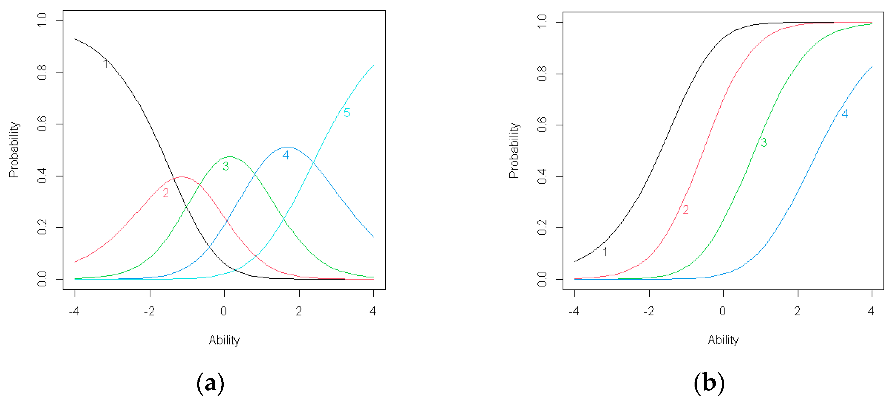
Symmetry 13 00223 g010
Figure 11. T(a) Item response category characteristic curves for C9; (b) Item operation characteristic curves for C9.
Symmetry 13 00223 g011
Figure 12. (a) Item response category characteristic curves for C10; (b) Item operation characteristic curves for C10.
Symmetry 13 00223 g012
Figure 13. (a) Item response category characteristic curves for C11; (b) Item operation characteristic curves for C11.
Symmetry 13 00223 g013
Figure 14. (a) Item response category characteristic curves for C12; (b) Item operation characteristic curves for C12.
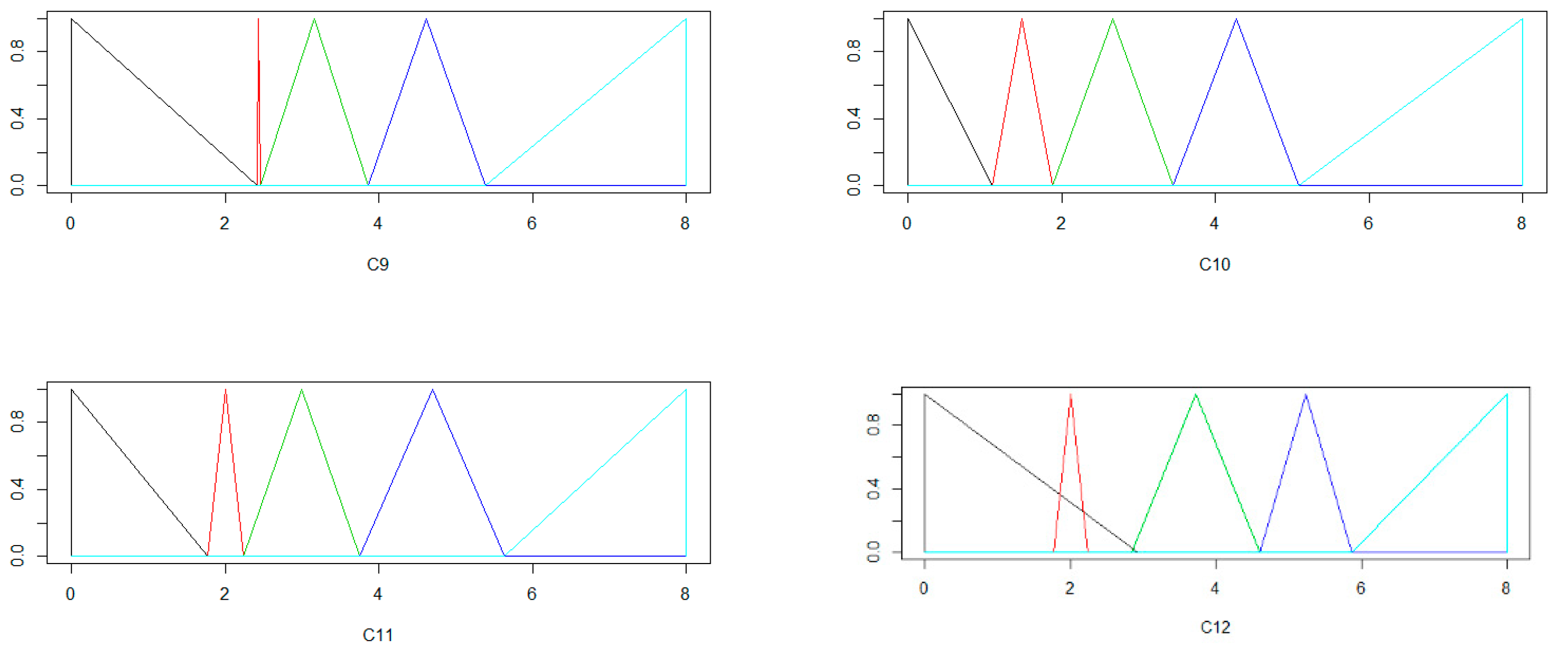
Symmetry 13 00223 g014
Figure 15. Triangular fuzzy numbers for criteria C1–C12.
Symmetry 13 00223 g015aSymmetry 13 00223 g015b
Figure 16. Box-plots for values of the fuzzy TOPSIS for (the first case).
Symmetry 13 00223 g016
Figure 17. Box-plots for values of the fuzzy TOPSIS for (the second case).
Symmetry 13 00223 g017
Table 1. Formulas for determining the parameters of triangular fuzzy numbers.
CategoryParameters of Triangular Fuzzy Numbers
a b c
VL−4−4 τ i 1
L τ i 1 τ i 1 + τ i 2 2 τ i 2
M τ i 2 τ i 2 + τ i 3 2 τ i 3
H τ i 3 τ i 3 + τ i 4 2 τ i 4
VH τ i 4 44
Table 2. The distribution of the research sample by place of residence.
Planned Sample SizeRealized Sample Size
Maximum Sampling Error Assumed = 3%Maximum Sampling Error Obtained = 3%
Total10471054
Commune A9795
Commune B107110
Commune C9798
Commune D242283
Commune E504468
Table 3. Thresholds for the Polychoric Correlation Model (PM) (for criteria C1–C6).
ThresholdsC1C2C3C4C5C6
1→2−1.270−1.110−0.980−1.280−0.820−1.970
2→3−0.597−0.352−0.231−0.5290.032−1.291
3→40.3230.5740.7140.4450.830−0.430
4→51.3101.5601.5601.4801.7300.620
Table 4. Thresholds for the PM (for criteria C7–C12).
ThresholdsC7C8C9C10C11C12
1→2−1.790−1.640−1.460−2.100−1.750−1.120
2→3−1.125−0.985−0.894−1.317−1.059−0.552
3→4−0.311−0.126−0.029−0.3140.0870.397
4→50.7800.8600.9800.7701.0601.310
Table 5. Thresholds for the Polytomous Rasch Model (PRM) (for criteria C1–C6).
ThresholdsC1C2C3C4C5C6
1→2−1.468−1.356−1.16−1.599−1.018−2.549
2→3−1.090.675−0.523−0.9680.033−1.991
3→40.4240.8081.1020.6251.103−0.771
4→51.9462.3802.2152.2842.6100.800
Table 6. Thresholds for the PRM (for criteria C7–C12).
ThresholdsC7C8C9C10C11C12
1→2−2.268−2.000−1.589−2.911−2.225−1.081
2→3−1.707−1.584−1.545−2.121−1.764−1.157
3→4−0.651−0.287−0.145−0.549−0.2440.598
4→51.1141.1751.3841.0881.6321.868
Table 7. Thresholds for the Rating Scale Model (RSM) (for criteria C1–C6).
ThresholdsC1C2C3C4C5C6
1→2−1.463−1.142−0.986−1.342−0.724−2.503
2→3−0.927−0.606−0.450−0.806−0.188−1.967
3→40.3860.7070.8640.5081.125−0.653
4→51.8392.1602.3161.9602.5780.799
Table 8. Thresholds for the RSM (for criteria C7–C12).
ThresholdsC7C8C9C10C11C12
1→2−2.284−2.073−1.911−2.375−2.020−1.368
2→3−1.748−1.537−1.376−1.839−1.484−0.832
3→4−0.435−0.224−0.062−0.525−0.1710.481
4→51.0181.2291.3910.9271.2821.934
Table 9. Thresholds for the Partial Credit Model (PCM) model (for criteria C1–C6).
ThresholdsC1C2C3C4C5C6
1→2−1.365−1.258−1.075−1.484−0.941−2.377
2→3−0.997−0.613−0.471−0.8830.041−1.838
3→40.4050.7631.0350.5921.041−0.702
4→51.8302.2392.0912.1472.4610.761
Table 10. Thresholds for the PCM model (for criteria C7–C12).
ThresholdsC7C8C9C10C11C12
1→2−2.113−1.863−1.483−2.711−2.072−1.009
2→3−1.573−1.458−1.419−1.955−1.622−1.056
3→4−0.589−0.254−0.122−0.498−0.2130.566
4→51.0511.1101.3051.0271.5321.761
Table 11. Thresholds for the Generalized Partial Credit Model (GPCM) model (for criteria C1–C6).
ThresholdsC1C2C3C4C5C6
1→2−1.366−1.283−1.107−1.583−1.076−2.317
2→3−1.026−0.661−0.542−1.0450.084−1.788
3→40.4080.8001.1440.6731.306−0.686
4→51.8652.3512.2382.4343.0860.747
Table 12. Thresholds for the GPCM model (for criteria C7–C12).
ThresholdsC7C8C9C10C11C12
1→2−1.916−1.747−1.455−2.560−2.026−0.960
2→3−1.320−1.253−1.120−1.815−1.577−1.456
3→4−0.444−0.212−0.086−0.467−0.2100.730
4→50.8870.9961.1080.9701.4952.131
Table 13. Thresholds for the Graded Response Model (GRM) model (for criteria C1–C6).
ThresholdsC1C2C3C4C5C6
1→2−1.739−1.648−1.506−2.036−1.462−2.798
2→3−0.795−0.523−0.365−0.8200.049−1.777
3→40.4500.8261.0400.6761.448−0.575
4→51.8422.3802.4352.4103.2470.838
Table 14. Thresholds for the GRM model (for criteria C7–C12).
ThresholdsC7C8C9C10C11C12
1→2−2.139−2.000−1.701−2.916−2.457−1.839
2→3−1.308−1.168−1.030−1.766−1.439−0.942
3→4−0.335−0.129−0.037−0.422−0.1110.545
4→50.8971.0211.1091.0211.4542.088
Table 15. Thresholds for the Nominal Response Model (NRM) model (for criteria C1–C6).
ThresholdsC1C2C3C4C5C6
1→2−1.371−1.559−1.280−1.533−1.130−2.374
2→3−1.203−0.973−0.791−1.416−0.454−2.505
3→4−0.598−0.318−0.158−0.6350.038−1.518
4→5−0.0960.3890.5390.1970.891−0.924
Table 16. Thresholds for the NRM model (for criteria C7–C12).
ThresholdsC7C8C9C10C11C12
1→2−2.053−1.855−1.541−2.707−2.7880.692
2→3−1.628−1.504−1.370−2.577−2.059−1.898
3→4−1.136−0.993−0.779−1.622−1.220−0.455
4→5−0.732−0.608−0.357−0.859−0.4720.438
Table 17. Parameters of triangular fuzzy numbers estimated on the basis of the PM (for criteria C1–C6).
CategoryFuzzy Number ParametersCriteria
C1C2C3C4C5C6
1—VLa0.0000.0000.0000.0000.0000.000
b0.0000.0000.0000.0000.0000.000
c2.7302.8903.0202.7203.1802.030
2—La2.7302.8903.0202.7203.1802.030
b3.0673.2693.3953.0963.6062.370
c3.4033.6483.7693.4714.0322.709
3—Ma3.4033.6483.7693.4714.0322.709
b3.8634.1114.2423.9584.4313.140
c4.3234.5744.7144.4454.8303.570
4—Ha4.3234.5744.7144.4454.8303.570
b4.8175.0675.1374.9635.2804.095
c5.3105.5605.5605.4805.7304.620
5—VHa5.3105.5605.5605.4805.7304.620
b8.0008.0008.0008.0008.0008.000
c8.0008.0008.0008.0008.0008.000
Table 18. Parameters of triangular fuzzy numbers estimated on the basis of the PM (for criteria C7–C12).
CategoryFuzzy Number ParametersCriteria
C7C8C9C10C11C12
1—VLa0.0000.0000.0000.0000.0000.000
b0.0000.0000.0000.0000.0000.000
c2.2102.3602.5401.9002.2502.880
2—La2.2102.3602.5401.9002.2502.880
b2.5432.6882.8232.2922.5963.164
c2.8753.0153.1062.6832.9413.448
3—Ma2.8753.0153.1062.6832.9413.448
b3.2823.4453.5393.1853.5143.923
c3.6893.8743.9713.6864.0874.397
4—Ha3.6893.8743.9713.6864.0874.397
b4.2354.3674.4764.2284.5744.854
c4.7804.8604.9804.7705.0605.310
5—VHa4.7804.8604.9804.7705.0605.310
b8.0008.0008.0008.0008.0008.000
c8.0008.0008.0008.0008.0008.000
Table 19. Parameters of triangular fuzzy numbers estimated on the basis of the PRM (for criteria C1–C6).
CategoryFuzzy Number ParametersCriteria
C1C2C3C4C5C6
1—VLa0.0000.0000.0000.0000.0000.000
b0.0000.0000.0000.0000.0000.000
c2.5322.6442.8402.4012.9821.451
2—La2.5322.6442.8402.4012.9821.451
b2.7213.6603.1592.7173.5081.730
c2.9104.6753.4773.0324.0332.009
3—Ma2.9104.6753.4773.0324.0332.009
b3.6674.7424.2903.8294.5682.619
c4.4244.8085.1024.6255.1033.229
4—Ha4.4244.8085.1024.6255.1033.229
b5.1855.5945.6595.4555.8574.015
c5.9466.3806.2156.2846.6104.800
5—VHa5.9466.3806.2156.2846.6104.800
b8.0008.0008.0008.0008.0008.000
c8.0008.0008.0008.0008.0008.000
Table 20. Parameters of triangular fuzzy numbers estimated on the basis of the PRM (for criteria C7–C12).
CategoryFuzzy Number ParametersCriteria
C7C8C9C10C11C12
1—VLa0.0000.0000.0000.0000.0000.000
b0.0000.0000.0000.0000.0000.000
c1.7322.002.4111.0891.7752.919
2—La1.7322.002.4111.0891.7752.919
b2.0132.2082.4331.4842.0062.881
c2.2932.4162.4551.8792.2362.843
3—Ma2.2932.4162.4551.8792.2362.843
b2.8213.0653.1552.6652.9963.721
c3.3493.7133.8553.4513.7564.598
4—Ha3.3493.7133.8553.4513.7564.598
b4.2324.4444.6204.2704.6945.233
c5.1145.1755.3845.0885.6325.868
5—VHa5.1145.1755.3845.0885.6325.868
b8.0008.0008.0008.0008.0008.000
c8.0008.0008.0008.0008.0008.000
Table 21. Parameters of triangular fuzzy numbers estimated on the basis of the RSM (for criteria C1–C6).
CategoryFuzzy Number ParametersCriteria
C1C2C3C4C5C6
1—VLa0.0000.0000.0000.0000.0000.000
b0.0000.0000.0000.0000.0000.000
c2.5372.8583.0142.6583.2761.497
2—La2.5372.8583.0142.6583.2761.497
b2.8053.1263.2822.9263.5441.765
c3.0733.3943.5503.1943.8122.033
3—Ma3.0733.3943.5503.1943.8122.033
b3.7304.0504.2073.8514.4692.690
c4.3864.7074.8644.5085.1253.347
4—Ha4.3864.7074.8644.5085.1253.347
b5.1135.4335.5905.2345.8524.073
c5.8396.1606.3165.9606.5784.799
5—VHa5.8396.1606.3165.9606.5784.799
b8.0008.0008.0008.0008.0008.000
c8.0008.0008.0008.0008.0008.000
Table 22. Parameters of triangular fuzzy numbers estimated on the basis of the RSM (for criteria C7–C12).
CategoryFuzzy Number ParametersCriteria
C7C8C9C10C11C12
1—VLa0.0000.0000.0000.0000.0000.000
b0.0000.0000.0000.0000.0000.000
c1.7161.9272.0891.6251.9802.632
2—La1.7161.9272.0891.6251.9802.632
b1.9842.1952.3571.8932.2482.900
c2.2522.4632.6242.1612.5163.168
3—Ma2.2522.4632.6242.1612.5163.168
b2.9083.1193.2812.8183.1723.825
c3.5653.7763.9383.4753.8294.481
4—Ha3.5653.7763.9383.4753.8294.481
b4.2914.5024.6644.2014.5555.208
c5.0185.2295.3914.9275.2825.934
5—VHa5.0185.2295.3914.9275.2825.934
b8.0008.0008.0008.0008.0008.000
c8.0008.0008.0008.0008.0008.000
Table 23. Parameters of triangular fuzzy numbers estimated on the basis of the PCM (for criteria C1–C6).
CategoryFuzzy Number ParametersCriteria
C1C2C3C4C5C6
1—VLa0.0000.0000.0000.0000.0000.000
b0.0000.0000.0000.0000.0000.000
c2.6352.7422.9252.5163.0591.623
2—La2.6352.7422.9252.5163.0591.623
b2.8193.0653.2272.8163.5501.893
c3.0033.3873.5293.1174.0412.162
3—Ma3.0033.3873.5293.1174.0412.162
b3.7044.0754.2823.8544.5412.730
c4.4054.7635.0354.5925.0413.298
4—Ha4.4054.7635.0354.5925.0413.298
b5.1185.5015.5635.3695.7514.029
c5.8306.2396.0916.1476.4614.761
5—VHa5.8306.2396.0916.1476.4614.761
b8.0008.0008.0008.0008.0008.000
c8.0008.0008.0008.0008.0008.000
Table 24. Parameters of triangular fuzzy numbers estimated on the basis of the PCM (for criteria C7–C12).
CategoryFuzzy Number ParametersCriteria
C7C8C9C10C11C12
1—VLa0.0000.0000.0000.0000.0000.000
b0.0000.0000.0000.0000.0000.000
c1.8872.1372.5171.2891.9282.991
2—La1.8872.1372.5171.2891.9282.991
b2.1572.3402.5491.6672.1532.968
c2.4272.5422.5812.0452.3782.944
3—Ma2.4272.5422.5812.0452.3782.944
b2.9193.1443.2302.7743.0823.755
c3.4113.7463.8783.5023.7874.566
4—Ha3.4113.7463.8783.5023.7874.566
b4.2314.4284.5924.2654.6605.163
c5.0515.1105.3055.0275.5325.761
5—VHa5.0515.1105.3055.0275.5325.761
b8.0008.0008.0008.0008.0008.000
c8.0008.0008.0008.0008.0008.000
Table 25. Parameters of triangular fuzzy numbers estimated on the basis of the GPCM (for criteria C1–C6).
CategoryFuzzy Number ParametersCriteria
C1C2C3C4C5C6
1—VLa0.0000.0000.0000.0000.0000.000
b0.0000.0000.0000.0000.0000.000
c2.6342.7172.8932.4172.9241.683
2—La2.6342.7172.8932.4172.9241.683
b2.8043.0283.1762.6863.5041.948
c2.9743.3393.4582.9554.0842.212
3—Ma2.9743.3393.4582.9554.0842.212
b3.6914.0704.3013.8144.6952.763
c4.4084.8005.1444.6735.3063.314
4—Ha4.4084.8005.1444.6735.3063.314
b5.1375.5765.6915.5536.1964.030
c5.8656.3516.2386.4347.0864.747
5—VHa5.8656.3516.2386.4347.0864.747
b8.0008.0008.0008.0008.0008.000
c8.0008.0008.0008.0008.0008.000
Table 26. Parameters of triangular fuzzy numbers estimated on the basis of the GPCM (for criteria C7–C12).
CategoryFuzzy Number ParametersCriteria
C7C8C9C10C11C12
1—VLa0.0000.0000.0000.0000.0000.000
b0.0000.0000.0000.0000.0000.000
c2.0842.2532.5451.4401.9743.040
2—La2.0842.2532.5451.4401.9743.040
b2.3822.5002.7131.8122.1982.792
c2.6802.7472.8802.1852.4232.544
3—Ma2.6802.7472.8802.1852.4232.544
b3.1183.2683.3972.8593.1073.637
c3.5563.7883.9143.5333.7904.730
4—Ha3.5563.7883.9143.5333.7904.730
b4.2214.3924.5114.2514.6435.430
c4.8874.9965.1084.9705.4956.131
5—VHa4.8874.9965.1084.9705.4956.131
b8.0008.0008.0008.0008.0008.000
c8.0008.0008.0008.0008.0008.000
Table 27. Parameters of triangular fuzzy numbers estimated on the basis of the NRM (for criteria C1–C6).
CategoryFuzzy Number ParametersCriteria
C1C2C3C4C5C6
1—VLa0.0000.0000.0000.0000.0000.000
b0.0000.0000.0000.0000.0000.000
c2.6292.4412.7202.4672.8701.626
2—La2.6292.4412.7202.4672.8701.626
b2.7132.7342.9642.5263.2081.560
c2.7973.0273.2092.5843.5461.495
3—Ma2.7973.0273.2092.5843.5461.495
b3.0993.3553.5262.9753.7921.988
c3.4023.6823.8423.3654.0382.482
4—Ha3.4023.6823.8423.3654.0382.482
b3.6534.0354.1913.7814.4652.779
c3.9044.3894.5394.1974.8913.076
5—VHa3.9044.3894.5394.1974.8913.076
b8.0008.0008.0008.0008.0008.000
c8.0008.0008.0008.0008.0008.000
Table 28. Parameters of triangular fuzzy numbers estimated on the basis of the NRM (for criteria C7–C12).
CategoryFuzzy Number ParametersCriteria
C7C8C9C10C11C12
1—VLa0.0000.0000.0000.0000.0000.000
b0.0000.0000.0000.0000.0000.000
c1.9472.1452.4591.2931.2124.692
2—La1.9472.1452.4591.2931.2124.692
b2.1602.3212.5451.3581.5763.397
c2.3722.4962.6301.4231.9412.102
3—Ma2.3722.4962.6301.4231.9412.102
b2.6182.7512.9261.9002.3602.824
c2.8643.0073.2212.3782.7803.545
4—Ha2.8643.0073.2212.3782.7803.545
b3.0663.1993.4322.7603.1543.992
c3.2683.3923.6433.1413.5284.438
5—VHa3.2683.3923.6433.1413.5284.438
b8.0008.0008.0008.0008.0008.000
c8.0008.0008.0008.0008.0008.000
Table 29. Parameters of triangular fuzzy numbers estimated on the basis of the GRM (for criteria C1–C6).
CategoryFuzzy Number ParametersCriteria
C1C2C3C4C5C6
1—VLa0.0000.0000.0000.0000.0000.000
b0.0000.0000.0000.0000.0000.000
c2.2612.3522.4941.9642.5381.202
2—La2.2612.3522.4941.9642.5381.202
b2.7332.9143.0652.5723.2931.713
c3.2053.4773.6353.1804.0492.223
3—Ma3.2053.4773.6353.1804.0492.223
b3.8274.1514.3383.9284.7492.824
c4.4504.8265.0404.6765.4483.425
4—Ha4.4504.8265.0404.6765.4483.425
b5.1465.6035.7375.5436.3484.132
c5.8426.3806.4356.4107.2474.838
5—VHa5.8426.3806.4356.4107.2474.838
b8.0008.0008.0008.0008.0008.000
c8.0008.0008.0008.0008.0008.000
Table 30. Parameters of triangular fuzzy numbers estimated on the basis of the GRM (for criteria C7–C12).
CategoryFuzzy Number ParametersCriteria
C7C8C9C10C11C12
1—VLa0.0000.0000.0000.0000.0000.000
b0.0000.0000.0000.0000.0000.000
c1.8612.0002.2991.0841.5432.161
2—La1.8612.0002.2991.0841.5432.161
b2.2772.4162.6341.6592.0522.609
c2.6922.8322.9702.2342.5613.058
3—Ma2.6922.8322.9702.2342.5613.058
b3.1793.3523.4672.9063.2253.801
c3.6653.8713.9633.5783.8894.545
4—Ha3.6653.8713.9633.5783.8894.545
b4.2814.4464.5364.3004.6715.316
c4.8975.0215.1095.0215.4546.088
5—VHa4.8975.0215.1095.0215.4546.088
b8.0008.0008.0008.0008.0008.000
c8.0008.0008.0008.0008.0008.000
Table 31. The values of the fuzzy Technique for Order of Preference by Similarity to Ideal Solution (TOPSIS).
CommunesFuzzy TOPSIS Rating
PMPRMRSMPCMGPCMGRMNRM
A0.6260.6040.6040.6070.6070.6060.6114
B0.6440.6230.6250.6240.6240.6250.6233
C0.6670.6480.6510.6500.6490.6510.6452
D0.6890.6740.6760.6750.6740.6760.6701
E0.6000.5780.5820.5810.5800.5780.5895
Table 32. Fuzzy conversion scales for comparative analysis.
Fuzzy Conversion Scale CS1 [12]Fuzzy Conversion Scale CS2 [10]
Triangular fuzzy number Triangular fuzzy number
CategoryabcCategoryabc
Terrible0.10.10.2Very low000.2
Bad0.20.30.4Low00.20.4
Normal0.40.50.6Fair0.30.50.7
Good0.60.70.8High0.60.81
Superb0.80.90.9Very high0.811
Fuzzy conversion scale CS3 [14]Fuzzy conversion scale CS4 [16]
CategoryabcCategoryabc
Very poor001Very poor013
Poor013Poor135
Fair357Fair357
Good7910Good579
Very good91010Very good7910
Fuzzy conversion scale CS5 [17]
Categoryabc
Very low113
Low135
Medium357
High579
Very high799
Publisher’s Note: MDPI stays neutral with regard to jurisdictional claims in published maps and institutional affiliations.

