Abstract
Evaluation of online teaching quality has become an important issue because many universities are turning to online classes due to the Corona Virus Disease 2019 (COVID-19) pandemic. In this paper, online teaching quality evaluation is considered as a linguistic multi-attribute group decision-making (MAGDM) problem. Generally, the evaluation sematic information can be symmetrically or asymmetrically distributed in linguistic term sets. Thus, an extended linguistic MAGDM framework is proposed for evaluating online teaching quality. As the main contribution, the proposed method takes into account the risk preferences of assessment experts (AEs) and unknown weight information of attributes and sub-attributes. To be specific, the Delphi method is employed to establish a multi-level evaluation indicator system (EIS) of online teaching quality. Then, by introducing the group generalized linguistic term set (GLTS) with two risk preference parameters, a two-stage optimization model is developed to calculate the weights of attributes and sub-attributes objectively. Subsequently, the linguistic MAGDM framework was divided into two stages. The first stage maximizes the group comprehensive rating values of teachers on different attributes to obtain partial ranking results for teachers on each attribute. The latter stage maximizes the group comprehensive rating values of teachers to evaluate the overall quality. Finally, a case study is provided to illustrate how to apply the framework to evaluate online teaching quality.
1. Introduction
Due to the outbreak of Corona Virus Disease 2019 (COVID-19), universities in many countries have adopted online teaching methods to prevent the spread of the epidemic on campus. According to data published by the United Nations Educational, Scientific and Cultural Organization (UNESCO), as of 28 April 2020, 168 countries worldwide had closed their campuses due to the epidemic and have adopted online teaching methods [1]. From the Chinese Ministry of Education, as of 8 May, 1454 colleges and universities nationwide were conducting online teaching, 1.03 million teachers were offering 1.07 million courses online, and a total of 17.75 million college students had participated in online learning. Currently, the global epidemic situation is still grim, and online teaching will continue to be one of the primary forms, especially in universities where students come from a wide variety of regions [2].
Large-scale online teaching has effectively solved the problem of students learning at home, but the changing of teaching environment from offline to online has also posed significant challenges to teaching quality. For instance, the changing scenarios and the lack of a sense of presence make it difficult for teachers and students to interact effectively. Meanwhile, network congestion occurs frequently when a large number of students attend the classes at the same time. Against this backdrop, how to assess and promote the quality of online teaching has become a key issue for education departments and universities. To this end, exploring and constructing scientific and rational indicators and scientific methods for assessing the quality of online teaching plays a crucial role in improving the online teaching quality [1,3].
To the best of knowledge, the complexity of teaching quality assessment leads to an evaluation process involving multiple levels of indicators and numerous assessment experts (AEs). Thus, the issue of assessing the quality of online teaching can also be regarded as a multi-attribute group decision-making (MAGDM) problem. In practical teaching evaluation problems, the choice of evaluation indicator system (EIS) and the evaluation method is related to the quality of evaluation results. The EISs are generally divided into two categories: single-level EISs [4,5,6,7] and multi-level EISs [8,9,10,11,12,13]. Additionally, there are many kinds of evaluation methods, such as the grey relational coefficient embed to the technique for order of preference by similarity to an ideal solution (Grey-TOPSIS) [4], analytic hierarchy process (AHP) [8,10,12,13], fuzzy comprehensive evaluation (FCE) [5,8,11,13], characteristic objects methods [6,7], cloud model [9] and so on. For example, Song and Zheng [4] combined the grey correlation with TOPSIS methods to construct a new model for assessing the quality of teaching in universities. Faizi et al. [6] extended the characteristic objects method to solve MAGDM problem in a hesitant fuzzy environment. Faizi et al. [7] further proposed a new MAGDM method by combining the characteristic object method and triangular intuitionistic fuzzy numbers, which is different from the hesitant fuzzy environment. Chen et al. [8] proposed an evaluation framework based on fuzzy AHP and FCE methods, and established a teaching performance indicator evaluation system to improve teaching performance of teachers, which is the primary means to improving the teaching quality of teachers. Chang and Wang [9] assessed teachers in higher education by constructing the interval cloud evaluation matrix and determining the order of importance of the decision program based on the cloud model. Wang [11] proposed a new data mining algorithm and established an improved FCE method to deal with the evaluation problem of physical education. Obviously, to ensure the accuracy of evaluation results, a growing number of evaluation problems need to be assessed with multi-level EISs.
According to the existing literature on teaching quality evaluation, there are two gaps need to be filled. The first is the lack of a multi-level EIS based on online teaching quality evaluation. The second is that the evaluation processes mentioned above did not take into account the influence of AEs’ risk preferences on linguistic evaluation information.
As to the selection of indicators for teaching quality evaluation, Song and Zheng [4] investigated the indicator system for assessing the quality of teaching in traditional classrooms, which was constructed from the perspectives of teaching plans, teaching methods, communication skills, and teaching professional level, and then assessed the quality of teaching in five universities. Yang et al. [13] evaluated the quality of the basic nursing course at Peking University in terms of teaching attitudes, teaching environment, teaching content, and teaching feedback. Kong et al. [14] constructed indicators for assessing teaching quality from the dimensions of attitude, content, teaching art, classroom management, and teaching effectiveness. Peng and Dai [15] assessed the classroom teaching quality of teachers in terms of the dimensions of teaching capacity, teaching attitude, teaching content, teaching method, and teaching effect. These researches provide a reference for this paper to build a new multi-level EIS of online teaching evaluation.
In addition, in the process of online teaching evaluation, due to the complexity of the evaluation problem and the limited knowledge of AEs, it is easier for them to give evaluation information in the form of linguistic terms on the teachers with regard to each sub-attribute. In order to allow linguistic terms to be aggregated and compared, scholars have carried out semantic representations of linguistic terms. Herrera and Martínez [16] proposed a 2-tuple linguistic representation model to represent semantic values of linguistic terms in a balanced linguistic term set (LTS) and represented the linguistic term as a linguistic 2-tuple. Wang and Hao [17] presented a new proportional 2-tuple linguistic representation model to compute with words in an unbalanced LTS. Dong et al. [18] defined the concept of the numerical scale, and on this basis, extended the 2-tuple linguistic representation model to compute with words in an unbalanced LTS. Subsequently, Rodriguez et al. [19] introduced the concept of a hesitant fuzzy LTS, which provided a linguistic and computational basis to increase the richness of linguistic elicitation. Dong et al. [20] proposed a novel computing with words method to construct the hesitant fuzzy LTS by using an unbalanced LTS and the numerical scale. Li et al. [21] presented a personalized individual semantics model to personalize individual semantics by the 2-tuple linguistic model and an interval numerical scale. Liu et al. [22] proposed a new fuzzy envelope for the hesitant fuzzy LTS in form of type-2 fuzzy sets for representing comparative linguistic expressions in decision contexts, which overcomes the limitation of existing representations in dealing with inherent uncertainties. However, in actual online teaching evaluation, different AEs may have different expectations for semantic values of linguistic terms, which can be described by their risk preferences [23]. Therefore, it is necessary to investigate the linguistic representation model in linguistic MAGDM problems based on risk preferences.
With regard to linguistic MAGDM based on risk preferences, Zhou and Xu [24] extended the sigmoid function and presented the concept of a generalized linguistic term set (GLTS). They applied it to linguistic multi-attribute decision making involving risk preferences. Lin and Wang [23] presented the concept of GLTSs with triangular fuzzy semantic values, and developed a new method for coping with linguistic MADM problems considering decision makers’ risk preferences. Lin and Wang [25] developed a new framework to solve the linguistic MAGDM problem based on risk preferences, where attribute evaluation values are represented by linguistic terms and the attribute weight information is incomplete. Guo and Sun [26] combined single-valued neutrosophic LTSs with prospect theory, and introduced a new comprehensive fuzzy decision approach to deal with linguistic MAGDM. Focusing on decision makers’ risk preferences and regret theory, Ma et al. [27] initiated an approach to solve the behavioral multi-attribute decision-making problem based on probability expressions. Liao et al. [28] launched a Choquet integral-based hesitant fuzzy gained and lost dominance score method based on prospect theory to deal with MAGDM problems with experts’ risk preference psychology. Obviously, the above methods and case studies are all based on a single-level EIS. This paper extends the linguistic MAGDM based on risk preferences to the context of a multi-level EIS.
Different from group decision problems with preference relations [29,30], the MAGDM problems involves the determination of attribute weights. To evaluate the quality of online teaching according to the given EIS, it is an important issue of whether to provide attribute weights. In fact, it is difficult for AEs to give attribute weight information in many cases. Thus, some scholars have conducted studies on this issue. For example, based on the standard deviation and average deviation of the interval type-2 fuzzy set, Gong [31] established an optimization model to calculate attribute weights in linguistic MAGDM, in which linguistic terms are transformed into interval type-2 fuzzy sets. Gupta et al. [32] proposed a new method for solving linguistic MAGDM problems, in which linguistic terms are converted into trapezoidal intuitionistic fuzzy numbers and Shannon’s entropy theory is used to determine attribute weights. Wang and Mendel [33] initiated a new method to deal with linguistic MAGDM problems based on interval type-2 fuzzy sets, where an optimization model is established to determine completely unknown attribute weights. Touqeer et al. [34] used a combination of grey relational analysis (GRA) method and projection method to calculate completely unknown attribute weights in linguistic MAGDM problems. We can see that these literatures are all based on the researches of linguistic MAGDM under the single-level EIS. Therefore, considering multi-level EIS and risk preferences, this paper develops a two-stage optimization model to derive the attribute weights and the sub-attribute weights.
In response to the above research deficiencies, this paper designs an extended framework to assess the quality of online teaching. The novelties of the framework are as follows:
- Taking into account the problem of online teaching quality evaluation, based on the existing traditional classroom teaching quality EISs [4,13,14,15], the Delphi method is employed to construct a brand-new multi-level EIS of online teaching quality, including five attributes and 15 sub-attributes.
- Inspired by the decision method in Lin and Wang [25], this framework extends the linguistic MAGDM method involving risk preferences from the single-level EIS to the multi-level one.
- In teaching quality evaluation problems based on multi-level EISs, many works of literature adopted the AHP approach to derive the weights of attributes and sub-attributes [8,9,10,11,12,13]. Sometimes AEs cannot make pairwise comparisons on the importance of attributes or sub-attributes, that is, they cannot use the AHP method to calculate attribute weights. Thus, based on the principle of maximizing the group comprehensive evaluation value of each alternative, a two-stage attribute and sub-attribute weight solution optimization model is established in this framework.
- The evaluation ranking results obtained by this framework are divided into the overall ranking result and partial ranking results, which are helpful for teachers and universities to understand their own situation and make targeted improvements.
The rest of this paper is structured as follows: Section 2 introduces the basic concepts related to LTSs, group GLTSs with individual risk preferences, the Euclidean distance between any two positive triangular fuzzy numbers, and the score function. Section 3 constructs a multi-level EIS for assessing online teaching quality of teachers, and then establishes a two-stage optimization model to solve the weights of attributes and sub-attributes in the EIS. Section 4 devises an extended evaluation framework and then describes the detailed evaluation process. Section 5 proposes a case study to verify the validity and feasibility of the proposed evaluation framework. Section 6 carries on the practical discussion to the evaluation ranking results including the overall and partial ranking results. Finally, Section 7 concludes this paper.
2. Preliminaries
In this section, we introduce some concepts about LTSs, group GLTSs, the Euclidean distance, and the score function.
2.1. Linguistic Term Set
Definition 1.
Reference [35]. Let be an LTS, where and are two positive integers, represents the granularity of the LTS , represents the central linguistic term, such as “medium” and “general”. If , then this LTS has the following properties:
- The LTSis ordered:if and only if;
- There is a negation operator:where.
If and the semantic information is symmetrically and uniformly distributed, then is called a balanced LTS; otherwise, is called an unbalanced LTS. For example, an LTS with seven granularities is denoted as follows:
2.2. Group Generalized Linguistic Term Set
2.2.1. Euclidean Distance
Definition 2.
Reference [36]. Let and be any two positive triangular fuzzy numbers, then the Euclidean distance between them is defined as
2.2.2. Score Function
For comparing and ranking triangular fuzzy numbers, assume that is a positive triangular fuzzy number, then its score function could be denoted as [37]
2.2.3. Group Generalized Linguistic Term Set Based on Risk Preferences
To describe the influence of the evaluation group’s risk preference on the semantic information of linguistic terms in an LTS, Lin and Wang [25] introduced the concept of a group GLTS.
Definition 3.
Reference [25]. Let be an LTS, then a group GLTS is denoted as follows:
where is a triangular fuzzy number with group risk preference parameters and , and represents a fuzzy semantic value of the linguistic term where . and are defined as
Obviously, for any , we have and . If , then the evaluation group tends to make a risk-seeking assessment. If , then the evaluation group tends to make a risk-neutral assessment. If , then the evaluation group tends to make a risk-averse assessment.
As for the symmetry of semantic information in the group GLTS , if and , then . This means that the semantic information is symmetrically distributed. Under this circumstance, if for , then follows a symmetric and approximately uniform distribution. Besides, if and , then . There also exists , so that , which means that follows an asymmetric and non-uniform distribution.
2.2.4. Determination of Risk Preference Parameters
In order to determine the group GLTS defined above, it is assumed that is an expected set of triangular fuzzy semantic values offered by the AE according to linguistic terms in the LTS . Then, an optimization model is constructed below:
where , and are decision variables, and denotes the Euclidean distance defined by (2).
By solving Equation (8), the values of the group risk preference parameters and are obtained. Then by plugging them into Equations (4)–(7), the group GLTS is derived.
3. EIS of Online Teaching Quality
3.1. Selection of Indicators for Evaluating the Online Teaching Quality
The selection of appropriate indicators is the fundamental to conducting the evaluation. In order to effectively identify the critical factors affecting the quality of teaching, the literature analysis and Delphi methods were used to construct indicators for evaluating the online teaching quality.
First, analysis of the existing literature reveals that in the traditional evaluation of teaching quality, scholars have focused on indicators of content, teaching methods, and effectiveness. Similarly, these indicators also could be selected for assessing online courses.
Then, through interviews with six teachers and 14 students who participated in online teaching, it was found that all interviewees focused on the classroom atmosphere in the online education process. Besides, the online teaching environment and the teaching platform were also key factors mentioned by the interviewees. Based on literature and interview research, this paper identified five attributes of the online teaching environment, online teaching platform, online teaching content and methods, online classroom climate, and online teaching effectiveness. These attributes were then decomposed to constitute 15 sub-attributes. Based on the literature study and interview research, this paper identified five primary indicators of online teaching environment, online teaching platform, online teaching content and methods, online classroom atmosphere, and online teaching effectiveness. Then, the primary indicators were decomposed to formulate 15 secondary indicators. Finally, the five primary indicators were treated as attributes and the secondary indicators were treated as sub-attributes . Sub-attributes represents a specific refinement of the attribute. In other words, the five attributes in this multi-level EIS contained 15 sub-attributes. The multi-level EIS is shown in Table 1 below.

Table 1.
The multi-level evaluation indicator system (EIS) of online teaching quality.
The attributes of the online teaching environment mainly refer to the external environmental requirements that support online education, including the network, hardware equipment, and teaching environment. The network environment requires the instructor to have a smooth network to ensure video and audio transmission when conducting instruction. Hardware equipment mainly refers to the teacher having the equipment to conduct online instruction, including computers, microphones, and cameras. Additionally, the physical environment primarily refers to space where classes are conducted without outside interference.
The online teaching platform requires that the online teaching system used by teachers and students be stable and easy to use. Personalized support requires the system to be able to sign in, take attendance, interact, and submit assignments. Different from the traditional teaching mode, the online platform plays the role of a “classroom” connecting students and teachers. Therefore, the stability of the online platform and personalized support functions are vital guarantees for the effective implementation of online teaching.
Regarding the content and methodological attributes of online teaching, teachers are required to teach comprehensive content and to highlight key points. The combination of theory and practice is also very crucial. Secondly, the teaching time is arranged in such a way that students can easily absorb and digest the course knowledge. It is also necessary to use a variety of teaching formats, such as a combination of live and recorded lectures, monologues and inspirational lectures. Unlike the traditional classroom teaching quality assessment, the content and methods for online teaching put forward higher requirements for universities and teachers. Specifically, teachers need to adjust teaching strategies, improve teaching methods, and optimize instructional design according to the needs of the scenario in order to compensate for the lack of presence and interaction resulting from online teaching.
The online classroom atmosphere contains the evaluation of teachers and students. Among them, the influence of teaching requires teachers to be full of energy, affable, use body language reasonably and appropriately, and teach in a natural and generous manner. The sub-attribute of student’s attitude requires students to have a right attitude towards learning and to pay attention to the class. Besides, the interaction and discussion between teacher and students is also an important basis for assessing the classroom atmosphere. This can be interpreted as a lively classroom atmosphere reflects the positive interaction between the teacher and the students and also makes the teacher more enthusiastic in teaching and helps the students to listen attentively to the lesson.
The teaching effectiveness is the reflection of the quality of instruction and can be used to measure if the teaching objectives are being met. This attribute includes if students master the content of the course in a timely and effective manner and whether the lectures inspire students to think. In addition, fostering creativity and improving problem-solving skills are also incorporated into this attribute.
Based on the above-detailed description of the evaluation indicators, for the sake of more intuitively understanding the MAGDM problems of online teaching quality evaluation, a multi-level hierarchic structure of online teaching quality evaluation composed of an objective, attributes, sub-attributes, and alternatives (teachers) is shown in Figure 1.
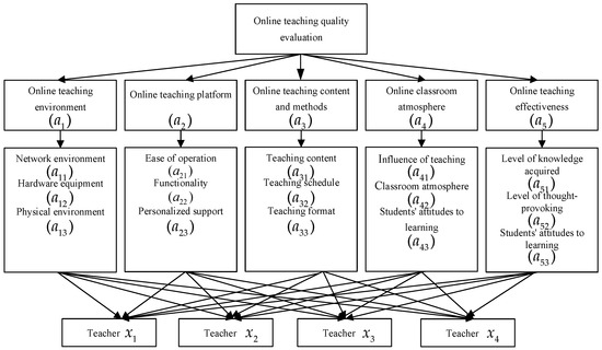
Figure 1.
The multi-level hierarchic structure of online teaching quality evaluation.
3.2. Determination of the Weights of Evaluation Indicators
Since this paper adopted a MAGDM approach to assess the online teaching quality of teachers, the determination of attribute weights was particularly vital. Obviously, the importance weights of different sub-attributes to the same attribute will also be different. Due to the limited knowledge of AEs and the complexity of evaluation problems, it may be difficult for them to give the weights of attributes and sub-attributes, that is, the weights of attributes and sub-attributes are completely unknown. It is supposed that represents the attribute weight vector containing attributes. means the sub-attribute weight vector, which contains sub-attributes under the attribute . and , and .
When the GLTS of the evaluation group is determined, the AE gives a linguistic-term-based decision matrix of the alternative over the sub-attribute under the attribute where , , , . Subsequently, each linguistic-term-based decision matrix can be converted into a triangular fuzzy decision matrix expressed by
where
Based upon triangular fuzzy decision matrices , assuming that the importance weight vector of AEs is , and . Then a triangular fuzzy weighted average operator and the AEs’ weight vector are utilized to aggregate individual triangular fuzzy decision matrices related to the attribute into a group one as follows:
where
Next, combining the sub-attribute weight vector and applying a triangular fuzzy weighted average operator, the triangular fuzzy evaluation values in the elements of the row in can be aggregated into a group comprehensive evaluation value for the alternative over the attribute , denoted by , namely:
Once is obtained, according to the attribute weight vector and the triangular fuzzy weighted average operator, the group comprehensive evaluation value of the alternative can be determined, that is
Since both and are completely unknown in this paper, thus, a two-stage optimization model is constructed to determine the weights of attributes and sub-attributes, shown as follows:
Stage 1:
As mentioned in Equation (13), represents the group comprehensive evaluation value for the alternative with respect to the attribute , the larger represents the better the alternative with regard to the attribute , which leads to a better alternative . Therefore, based on Equation (3), we first need to find the sub-attribute weight vector , so that is maximized for the alternative with respect to the attribute for all , . Thus, a multi-objective optimization model in this stage is constructed as follows:
As for the attribute , each alternative is feasible and non-inferior, and the optimization model of each alternative has the same constraint conditions. Therefore, the aforementioned multi-objective optimization model can be transformed into an aggregated optimization model by setting the same sub-attribute weights for each alternative under the same attribute as follows:
Based on Equations (3) and (13), the optimization model (16) can be equivalently converted into
Solving the above optimization model (17) yields the optimal sub-attribute weight vector related to the attribute . The optimal solution of the model can be expressed as
Since the weight vector satisfies the constraint condition of unitization, it is also necessary to normalize , namely:
The optimal sub-attribute weight vector after normalization is obtained. Then, substituting into Equation (13), the optimal group comprehensive evaluation value of the alternative over the attribute is obtained by
Stage 2:
Once is determined, the larger the triangular fuzzy evaluation value , the better the alternative is. Similarly, based on Equation (3), we need to derive the attribute weight vector so that for any , is maximized. The following multi-objective optimization model of the second stage is constructed as
In the same way, the above multi-objective optimization model (21) is converted into an aggregated optimization model:
Based upon the score function of triangular fuzzy numbers, we substitute into Equation (14), and the optimization model (22) can be equivalently converted into:
Solving the optimization model (23) yields the optimal attribute weight vector . Then, utilize Equation (24) to normalize , the normalized attribute weight vector is derived by
Subsequently, substituting into Equation (14), and at the same time, according to Equation (20), the group comprehensive evaluation value of the alternative is calculated as
As the summary of this section, the brief flow of the two-stage optimization model used to solve the weights of attributes and sub-attributes is shown in Figure 2.
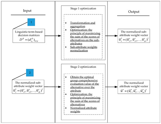
Figure 2.
The brief flow of the two-stage sub-attribute and attribute weight solving optimization model.
4. A Method for Linguistic MAGDM Involving Risk Preferences and Completely Unknown Weight Information
Taking into account linguistic MAGDM problems involving decision makers’ risk preferences, let be a set of alternatives, be a set of attributes, and be a set of sub-attributes related to the attribute . The weights of attributes and sub-attributes are completely unknown. Suppose that AEs represented by assess the alternative with regard to the sub-attribute to the attribute according to the LTS defined in Definition 1. Then they offer linguistic-term-based decision matrices as , where and the weights of AEs are known. Based on the risk preferences of AEs, a method for solving linguistic MAGDM problems with the completely unknown weights of attributes and sub-attributes is provided. The detailed evaluation process is described as follows:
Preprocessing:
Step 1: Based on the LTS , each AE assesses the alternative with regard to the sub-attribute relative to the attribute . The evaluation process could be expressed by linguistic-term-based decision matrices . Then, each AE provides his or her respective set of expected triangular fuzzy semantic values .
Step 2: Compute the group risk preference parameters and by solving the optimization model (8), and substitute them into Equations (4)–(7) to obtain the group GLTS .
Step 3: Transform decision matrices into triangular fuzzy decision matrices according to Equations (9) and (10).
Step 4: Utilize the triangular fuzzy weighted average operator to aggregate individual triangular fuzzy decision matrices into group triangular fuzzy decision matrices according to Equation (12).
Stage 1:
Step 5: Determine the normalized optimal sub-attribute weight vector by solving the nonlinear programming model (17) and using Equation (19) for normalization.
Step 6: Compute the optimal group comprehensive evaluation value for the alternative over the attribute according to Equation (20).
Step 7: Make use of Equation (3) to calculate scores .
Step 8: Obtain the ranking of all the alternatives over each attribute in descending order according to the size of scores , and use to indicate that is superior to with respect to the attribute .
Stage 2:
Step 9: Get the optimal attribute weight vector by solving the nonlinear programming model (23). Then employ Equation (24) to derive the normalized optimal one denoted by .
Step 10: Calculate the optimal group comprehensive evaluation value of each alternative in by making use of Equation (25).
Step 11: Generate scores of the optimal group comprehensive evaluation value for each alternative based on Equation (3).
Step 12: Assess and rank the alternatives in descending order according to the size of scores , and select the best alternative. Then, make use of to express that is preferred to , where .
Based on the detailed description of the above evaluation process, an extended framework of online teaching quality evaluation is devised in Figure 3.
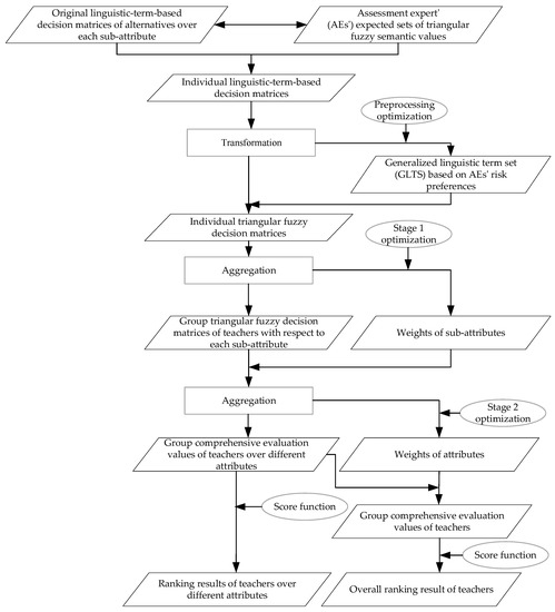
Figure 3.
The extended framework of online teaching quality evaluation.
5. A Case Study about Online Teaching Quality Evaluation
This section aims to provide a case to clarify the feasibility and effectiveness of the method and models presented in this paper.
5.1. Problem Description
During the outbreak of COVID-19, almost all universities across the countries postponed the opening of their classes. In order not to delay the progress of classroom teaching, a certain university requires teachers to teach students courses through online teaching. Because the online teaching method is relatively novel and unfamiliar to teachers, it is very crucial to control the quality of online teaching. For the sake of improving the quality of online teaching in this university, three AEs are invited to assess the online teaching quality of the four excellent teachers selected by the university. Then the best teacher is chosen to share his or her experience to improve the overall quality of online teaching in this university.
5.2. Evaluation of Online Teaching Quality among Four Teachers
Preprocessing:
Based upon the seven granular LTS presented in Definition 1 and the EIS of online teaching quality constructed in Table 1, the linguistic-term-based decision matrices are given by experts who assess four teachers with regard to fifteen sub-attributes by using linguistic terms in . The importance weight vector of experts are . The original linguistic-term-based decision matrices they provide are shown as follows:
Then, three experts give their own sets of triangular fuzzy semantic values they expected, expressed as follows:
As the importance weights of the three experts are 0.35, 0.25, and 0.4, respectively, solving the optimization model (8) yields the group risk preference parameters . Apparently, the group of AEs tend to make a risk-averse decision. Substituting the group risk preference parameters into Equations (4)–(7), the GLTS with seven granularities can be obtained as follows:
According to Equations (9) and (10), the above-mentioned linguistic-term-based decision matrices are transformed into triangular fuzzy decision matrices as follows:
According to Equations (11) and (12), the individual triangular fuzzy decision matrices are aggregated into group ones :
Stage 1:
Once the group triangular fuzzy decision matrices for the attribute are obtained, we can utilize Equation (19) to calculate the optimal normalized sub-attribute weight vector to the attribute :
Subsequently, based upon Equation (20), we can calculate the optimal group comprehensive evaluation value of the alternative over the attribute as
Next, according to Equation (3), the scores are computed as
For the attribute , we have , so the ranking result of teachers’ online teaching quality over the attribute is denoted by . In the same way, the ranking results of teachers’ online teaching quality over different attributes are obtained, as shown in Table 2.
Table 2.
Ranking results of teachers’ online teaching quality evaluation over different attributes.
Stage 2:
According to scores of the optimal group comprehensive evaluation value for the alternative with regard to the attribute obtained in Stage 1, the normalized optimal attribute weight vector is derived as by using Equation (24).
Based on Equation (25), we can calculate the optimal group comprehensive evaluation value of each alternative as
According to Equation (3), we can obtain the scores as
Because , the overall ranking result of four teachers is , which means that the teacher with the best online teaching quality is .
From the perspective of Table 2 and the overall ranking result, if the teacher with the best online teaching quality is chosen in terms of a certain attribute, then teacher is the best in aspects of online teaching platform and online teaching effectiveness. The teacher is better than other three teachers in terms of online teaching environment and atmosphere. The teacher has an absolute advantage in terms of online teaching content and methods. Compared with other teachers, although the teacher is not the best in every aspect, it almost always ranks in the second place, which is high and stable. On the contrary, the teacher ranks the worst in aspects of online teaching content and methods and online teaching effectiveness. The teacher has the worst ranking with respect to online teaching environment and platform. Except for the best ranking of the teacher in terms of the above-mentioned attributes, the first teacher ranks next to last for the other attributes, which indicates that teacher is at the lower end of the ranking and not stable in general. Although teachers , , and have the best online teaching quality among a certain attribute(s), in view of all the evaluation attributes, the teacher is the best.
6. Practical Discussion
The above-simulated case verifies the feasibility and effectiveness of the proposed evaluation framework. On the one hand, several inspirations to AEs are given by the evaluation process and results of the case. Initially, in the actual evaluation, AEs often have different expectations and considerations for semantic values of linguistic terms. Thus, the risk preference is used to describe and depict this phenomenon, which makes the evaluation results more accurate and persuasive. Meanwhile, we can find that the importance weights of attributes and sub-attributes in many multi-level EISs are subjectively given by AEs for previous evaluation researches. But in this paper, the importance weights of attributes and sub-attributes can be objectively derived through the proposed evaluation method. Therefore, it makes the evaluation process fairer and makes teachers more convincing. Next, from the evaluation results of the above case, we can see that there are not only the overall evaluation ranking result, but also partial ranking results of teachers over each attribute. This form of evaluation results can help universities and teachers better improve the quality of online teaching. For universities, they can not only select the best teacher in the overall ranking for teaching experience, but also choose the best one in a certain aspect to impart teaching experience in this aspect. For teachers, they can not only know their ranking in the comprehensive evaluation, but also understand their own deficiencies in some aspects to improve themselves.
On the other hand, the research in this paper also has some limitations, which need to be improved in the future. Firstly, this paper regards online teaching quality evaluation as a linguistic MAGDM problem, assuming that the AE group uses the same granular LTS for evaluation. In real life, because different AEs have different knowledge and different preferences, LTSs with different granularities may be employed by them for evaluation. How to convert LTSs with different granularities into ones with the same granularity under the consideration of individual AEs’ risk preferences is the direction of future research. Secondly, the form of evaluation information given in this paper is single. When different AEs give different types of evaluation information, how to transform and aggregate them is also the direction to be studied in the future. Thirdly, the proposed evaluation framework is applicable to online teaching quality evaluation, but it is also applicable to other application cases, which is worth further research in the future.
Of course, there are some other MAGDM methods that can be used to solve attribute weights, such as TOPSIS, VIKOR and PROMETHEE II methods [38]. Which method is suitable to be used in a realistic assessment environment should be measured by one or some benchmarks. In this paper, the online teaching evaluation process takes into account the risk preferences of AEs. However, the difference in risk preferences will affect the weights of attributes and sub-attributes in the EIS [23]. Thereby, in an evaluation environment that considers risk preferences, the presented attribute and sub-attribute weight solution optimization model and the devised evaluation framework are more suitable and applicable than some other MAGDM approaches.
7. Conclusions
In the current way of epidemic prevention and control, online teaching has gradually transformed into a mainstream learning method in universities. In order to ensure the quality of online teaching in universities, evaluation of online teaching quality is particularly important. By introducing and expanding the linguistic MAGDM method, this paper mainly copes with the evaluation problem of online teaching quality that considers AEs’ risk preferences and the completely unknown weights information in the multi-level EIS. Its contributions and advantages are manifested in four aspects. First of all, we construct a multi-level EIS of online teaching quality based upon the Delphi method, which can be well applied to evaluation of online teaching quality. Then, we extend Lin and Wang’s method [25] to apply to the evaluation problem based on a multi-level EIS which commonly exists in reality. Furthermore, according to the principle of maximizing the group comprehensive evaluation value of each alternative, we put forward the two-stage optimization model that can objectively solve the weights of attributes and sub-attributes. The presented two-stage optimization model has lower requirements for the AEs than other attribute solving models, and is more practical and objective. Lastly, in the process of evaluation, the evaluation results given by our framework include both the overall evaluation result and partial evaluation results. These evaluation results can help teachers and even universities to understand the specific problems existing in some aspects of current online teaching in more detail for timely improvement.
Author Contributions
Conceptualization, J.Y.; funding acquisition, J.Y.; methodology, H.L.; writing—original draft, H.L.; writing—review and editing, T.X. All authors have read and agreed to the published version of the manuscript.
Funding
This work is partially supported by the National Natural Science Foundation of China (Grant Nos. 71671125).
Acknowledgments
The authors are grateful to the editors and the anonymous reviewers for their constructive comments and suggestions which help us improve the quality of this article.
Conflicts of Interest
The authors declare no conflict of interest.
References
- Huang, R.; Liu, D.; Zhan, T. Guidance on Flexible Learning during Campus Closures: Ensuring Course Quality of Higher Education in COVID-19 Outbreak; Beijing Smart Learning Institute of Beijing Normal University: Beijing, China, 2020. [Google Scholar]
- Wang, X. Online Teaching Launched on a Massive Scale, this Year may Usher in the First Year of a New Wave of Change in Higher Education. Available online: http://www.whb.cn/zhuzhan/xue/20200521/349052.html (accessed on 21 May 2020).
- Zhang, X.; Wang, J.; Zhang, H.; Hu, J. A Heterogeneous Linguistic MAGDM Framework to Classroom Teaching Quality Evaluation. Eurasia J. Math. Sci. Technol. Educ. 2017, 13, 4929–4956. [Google Scholar] [CrossRef]
- Song, J.; Zheng, J.H. The Application of Grey-TOPSIS Method on Teaching Quality Evaluation of the Higher Education. Int. J. Emerg. Technol. Learn. 2015, 10, 42–45. [Google Scholar] [CrossRef]
- Ma, H.P. Research on Fuzzy Comprehensive Evaluation of Teaching Quality of College Public Physical Education based on Grey System Theory. Agro Food Ind. Hi-Tech 2017, 28, 2603–2607. [Google Scholar]
- Faizi, S.; Sałabun, W.; Rashid, T.; Watrobski, J.; Zafar, S. Group decision-making for hesitant fuzzy sets based on Characteristic Objects Method. Symmetry 2017, 9, 136. [Google Scholar] [CrossRef]
- Faizi, S.; Sałabun, W.; Rashid, T.; Zafar, S.; Watrobski, J. Intuitionistic fuzzy sets in multi-criteria group decision making problems using the Characteristic Objects Method. Symmetry 2020, 12, 1382. [Google Scholar] [CrossRef]
- Chen, J.F.; Hsieh, H.N.; Do, Q.H. Evaluating teaching performance based on fuzzy AHP and comprehensive evaluation approach. Appl. Soft. Comput. 2015, 28, 100–108. [Google Scholar] [CrossRef]
- Chang, T.C.; Wang, H. A Multi Criteria Group Decision-making Model for Teacher Evaluation in Higher Education Based on Cloud Model and Decision Tree. Eurasia J. Math. Sci. Technol. Educ. 2016, 12, 1243–1262. [Google Scholar] [CrossRef]
- Thanassoulis, E.; Dey, P.K.; Petridis, K.; Goniadis, I.; Georgiou, A.C. Evaluating higher education teaching performance using combined analytic hierarchy process and data envelopment analysis. J. Oper. Res. Soc. 2017, 68, 431–445. [Google Scholar] [CrossRef]
- Wang, Z.H. Fuzzy comprehensive evaluation of physical education based on high dimensional data mining. J. Intell. Fuzzy Syst. 2018, 35, 3065–3076. [Google Scholar] [CrossRef]
- Shen, L.Q.; Yang, J.; Jin, X.Y.; Hou, L.Y.; Shang, S.M.; Zhang, Y. Based on Delphi method and Analytic Hierarchy Process to construct the Evaluation Index system of nursing simulation teaching quality. Nurse Educ. Today 2019, 79, 67–73. [Google Scholar] [CrossRef]
- Yang, J.; Shen, L.Q.; Jin, X.Y.; Hou, L.Y.; Shang, S.M.; Zhang, Y. Evaluating the quality of simulation teaching in Fundamental Nursing Curriculum: AHP-Fuzzy comprehensive evaluation. Nurse Educ. Today 2019, 77, 77–82. [Google Scholar] [CrossRef] [PubMed]
- Kong, H.N.; Fan, H.J.; Zhao, Y.; Zhai, C.J.; Zhang, C.; Han, Y.J. Design of teaching quality evaluation model based on fuzzy mathematics and SVM algorithm. J. Intell. Fuzzy Syst. 2018, 35, 3091–3099. [Google Scholar]
- Peng, X.D.; Dai, J.G. Research on the assessment of classroom teaching quality with q-rung orthopair fuzzy information based on multiparametric similarity measure and combinative distance-based assessment. Int. J. Intell. Syst. 2019, 34, 1588–1630. [Google Scholar] [CrossRef]
- Herrera, F.; Martinez, L. A 2-tuple fuzzy linguistic representation model for computing with words. IEEE Trans. Fuzzy Syst. 2000, 8, 746–752. [Google Scholar]
- Wang, J.H.; Hao, J.Y. A new version of 2-tuple. fuzzy linguistic, representation model for computing with words. IEEE Trans. Fuzzy Syst. 2006, 14, 435–445. [Google Scholar] [CrossRef]
- Dong, Y.C.; Xu, Y.F.; Yu, S. Computing the Numerical Scale of the Linguistic Term Set for the 2-Tuple Fuzzy Linguistic Representation Model. IEEE Trans. Fuzzy Syst. 2009, 17, 1366–1378. [Google Scholar] [CrossRef]
- Rodriguez, R.M.; Martinez, L.; Herrera, F. Hesitant Fuzzy Linguistic Term Sets for Decision Making. IEEE Trans. Fuzzy Syst. 2012, 20, 109–119. [Google Scholar] [CrossRef]
- Dong, Y.C.; Li, C.C.; Herrera, F. Connecting the linguistic hierarchy and the numerical scale for the 2-tuple linguistic model and its use to deal with hesitant unbalanced linguistic information. Inf. Sci. 2016, 367, 259–278. [Google Scholar] [CrossRef]
- Li, C.C.; Dong, Y.C.; Herrera, F.; Herrera-Viedma, E.; Martinez, L. Personalized individual semantics in computing with words for supporting linguistic group decision making. An application on consensus reaching. Inf. Fusion 2017, 33, 29–40. [Google Scholar] [CrossRef]
- Liu, Y.Y.; Rodriguez, R.M.; Hagras, H.; Liu, H.B.; Qin, K.Y.; Martinez, L. Type-2 Fuzzy Envelope of Hesitant Fuzzy Linguistic Term Set: A New Representation Model of Comparative Linguistic Expression. IEEE Trans. Fuzzy Syst. 2019, 27, 2312–2326. [Google Scholar] [CrossRef]
- Lin, H.; Wang, Z.J. Linguistic multi-attribute decision making with considering decision makers’ risk preferences. J. Intell. Fuzzy Syst. 2017, 33, 1775–1784. [Google Scholar] [CrossRef]
- Zhou, W.; Xu, Z.S. Generalized asymmetric linguistic term set and its application to qualitative decision making involving risk appetites. Eur. J. Oper. Res. 2016, 254, 610–621. [Google Scholar] [CrossRef]
- Lin, H.; Wang, Z.J. Linguistic Multi-Attribute Group Decision Making with Risk Preferences and Its Use in Low-Carbon Tourism Destination Selection. Int. J. Environ. Res. Public Health 2017, 14, 1078. [Google Scholar] [CrossRef] [PubMed]
- Guo, Z.X.; Sun, F.F. Multi-attribute decision making method based on single-valued neutrosophic linguistic variables and prospect theory. J. Intell. Fuzzy Syst. 2019, 37, 5351–5362. [Google Scholar] [CrossRef]
- Ma, Z.Z.; Zhu, J.J.; Zhang, S.T. Probabilistic-based expressions in behavioral multi-attribute decision making considering pre-evaluation. Fuzzy Optim. Decis. Mak. 2020. [Google Scholar] [CrossRef]
- Liao, Z.Q.; Liao, H.C.; Tang, M.; Al-Barakati, A.; Llopis-Albert, C. A Choquet integral-based hesitant fuzzy gained and lost dominance score method for multi-criteria group decision making considering the risk preferences of experts: Case study of higher business education evaluation. Inf. Fusion 2020, 62, 121–133. [Google Scholar] [CrossRef]
- Bashir, Z.; Rashid, T.; Watrobski, J.; Sałabun, W.; Malik, A. Hesitant probabilistic multiplicative preference relations in group decision making. Appl. Sci. 2018, 8, 398. [Google Scholar] [CrossRef]
- Jin, F.; Garg, H.; Pei, L.; Liu, J.; Chen, H. Multiplicative consistency adjustment model and data envelopment analysis-driven decision-making process with probabilistic hesitant fuzzy preference relations. Int. J. Fuzzy Syst. 2020, 22, 2319–2332. [Google Scholar] [CrossRef]
- Gong, Y.B. Fuzzy Multi-Attribute Group Decision Making Method Based on Interval Type-2 Fuzzy Sets and Applications to Global Supplier Selection. Int. J. Fuzzy Syst. 2013, 15, 392–400. [Google Scholar]
- Gupta, P.; Mehlawat, M.K.; Grover, N. Intuitionistic fuzzy multi-attribute group decision-making with an application to plant location selection based on a new extended VIKOR method. Inf. Sci. 2016, 370, 184–203. [Google Scholar] [CrossRef]
- Wang, W.; Mendel, J.M. Multiple attribute group decision making with linguistic variables and complete unknown weight information. Iran J. Fuzzy Syst. 2019, 16, 145–157. [Google Scholar] [CrossRef]
- Touqeer, M.; Hafeez, A.; Arshad, M. Multi-attribute decision making using grey relational projection method based on interval type-2 trapezoidal fuzzy numbers. J. Intell. Fuzzy Syst. 2020, 38, 5979–5986. [Google Scholar] [CrossRef]
- Xu, Z.S. Deviation measures of linguistic preference relations in group decision making. Omega Int. J. Manag. Sci. 2005, 33, 249–254. [Google Scholar] [CrossRef]
- Chen, C.T. Extensions of the TOPSIS for group decision-making under fuzzy environment. Fuzzy Sets Syst. 2000, 114, 1–9. [Google Scholar] [CrossRef]
- Liou, T.S.; Wang, M.J.J. Ranking Fuzzy Numbers with Integral Value. Fuzzy Sets Syst. 1992, 50, 247–255. [Google Scholar] [CrossRef]
- Sałabun, W.; Watrobski, J.; Shekhovtsov, A. Are MCDA methods benchmarkable? A comparative study of TOPSIS, VIKOR, COPRAS, and PROMETHEE II methods. Symmetry 2020, 12, 1549. [Google Scholar] [CrossRef]
Publisher’s Note: MDPI stays neutral with regard to jurisdictional claims in published maps and institutional affiliations. |
© 2021 by the authors. Licensee MDPI, Basel, Switzerland. This article is an open access article distributed under the terms and conditions of the Creative Commons Attribution (CC BY) license (http://creativecommons.org/licenses/by/4.0/).