Inverse Maxwell Distribution and Statistical Process Control: An Efficient Approach for Monitoring Positively Skewed Process

Abstract

(1) Background: The literature discusses the inverse Maxwell distribution theoretically without application. Control charting is promising, but needs development for inverse Maxwell processes. (2) Methods: Thus, we develop the $V_{IM}$ control chart for monitoring the inverse Maxwell scale parameter and studied its statistical properties. The chart’s performance is evaluated using power curves and run length properties. (3) Results: Further, we use simulated data to compare the shift detection capability of our chart with Weibull, gamma, and lognormal charts. (4) Conclusion: The analysis demonstrates our chart’s efficiency for monitoring skewed processes. Finally, we apply our chart for monitoring real world lifetimes of car brake pads.

1. Introduction

In real-life, non-normal datasets are generated from various applied fields such as engineering, agricultural, and industrial sectors [1]. There are different but usual types of distributions available in statistics to model these non-normal datasets, but in real life, different kinds of situations arise where these types of popular distributions are not suitable. For this, we have to use other statistical distributions, including the inverse of usual distributions to fit the data. As a candidate of non-normal distribution, [2] proposed Maxwell distribution in life time modelling and studied its important distributional properties. This distribution is also used in chemistry, physics, as well as statistical mechanics [3,4,5]. Moreover, discrete Maxwell and Mixture Maxwell distributions are members of the Maxwell family of densities [6,7,8]. According to [9], the inverse of a distribution is less parsimonious than the real distribution. Hence, [10] derived inverse Maxwell distribution from the Maxwell distribution for enhancing its application fields and studied different statistical properties including moments, survival function, and parameter estimation. Later, they provided general and Bayesian estimators of a size-biased inverse Maxwell scale parameter [11,12]. Similarly, [10,13] studied the Bayes estimator of inverse Maxwell scale parameter by considering weighted quadratic loss function. However, none of the research mentioned offered any application of this distribution. The unavailability of some important statistical properties of this distribution as well as absence of its application motivate us to conduct the current study.

To determine whether or not a process is in control, a method called Statistical Process Control (SPC) conceived in 1920 by Walter A. Shewhart is applied [14]. SPC has various tools for evaluating a process and control chart is one of them [15]. Within these tools, control chart is more popular because it is a sophisticated technique to monitor variation or shift in a manufacturing process. It is extensively employed to detect the stability of process parameters and determine process capabilities in the agricultural, health, and industrial sectors [16]. The conventional control charts include the memory-less control charts and memory type charts. The Shewhart type control chart is usually considered as a memory-less control chart and is mostly used to detect transient cause variations which indicate large shifts in process parameters. It is based on the last sample information of any scheme, while the memory type charts accumulate total information in the entire series of sample observations to identify persistent cause variations. For a scheme based on either normal or non-normal distribution, the main parameters of the Shewhart chart are lower control limit (LCL), central line (CL), and upper control limit (UCL). The popularly applied kinds of memory control charts include exponentially weighted moving average (EWMA) and cumulative sum (CUSUM) control charts designed by Roberts [17] and Page [18], respectively. Most of these methods originate from large sample theory, which relies on asymptotic normality.

However, especially when sample sizes are not large, distribution specific control charts are more popular, reliable, and effective than the robust control charts for monitoring skewed processes among the scholars. Due to this, Hossain et al. [19,20] developed control charts named V chart and Maxwell CUSUM chart to monitor a Maxwell distribution’s parameter. Maxwell and Mixture Maxwell Cumulative Quantity control charts are also available in the literature for mixture Maxwell parameters [8]. Ref. [21] proposed a control chart for gamma distribution. Refs. [22,23] introduced Shewhart and EWMA type control charts using Rayleigh distribution for censored samples. Ref. [24] derived a control chart under lognormal distribution, namely the Lognormal S-chart. They suggested that their proposed chart outperforms existing charts for monitoring positively skewed process. However, the inverse Maxwell is another positively skewed non-normal distribution without any control chart application so far, and has a Galton skewness measure of 0.2578. (Galton index is a skewness measure that does not utilize the third moment and has a range of (−1, 1) with 0 signifying symmetry and a positive value indicating a longer right tail).

Ref. [25] studied the survival times for some breast cancer patients and reported that the survival times follow an inverse Maxwell distribution. The data set in [25] contains 121 patients with abnormal growth of breast cells beyond their usual boundaries. Since this is the most frequent type of cancer among women, fast detection of cancer cells is important. Thus, [25] also developed a EWMA chart to ensure fast detection of breast cancer cells for timely treatment of patients. Although [25] developed a EWMA control chart for the inverse Maxwell process, we have yet to find in the literature a Shewhart control chart to monitor the inverse Maxwell parameter where its suitability for monitoring positively skewed process is discussed.

In this article, we develop a control chart for the inverse Maxwell parameter and study its distributional properties. The outline of this article is as follows. Section 2.1 contains the densities of inverse Maxwell distribution as well as some unpublished characteristics such as entropy and fisher information. In Section 2.2, we develop a theoretical process to monitor the inverse Maxwell scale parameter, which we name as $V_{IM}$ control chart. We use various performance measurement tools to inspect the suitability of the $V_{IM}$ control chart for monitoring the inverse Maxwell parameter in Section 3.1. Then, to illustrate, the control chart has been implemented with a simulation study and real-life example in Section 3.2 and Section 3.4, respectively. In particular, the comparison of the proposed chart with existing control charts under simulated data and run length properties are presented in these sections and Section 3.3. Finally, Section 4 concludes this article and provides some general recommendations.

2. Material and Method

To investigate the properties and performance of the proposed chart, we discuss the method and supporting material for development of the chart here.

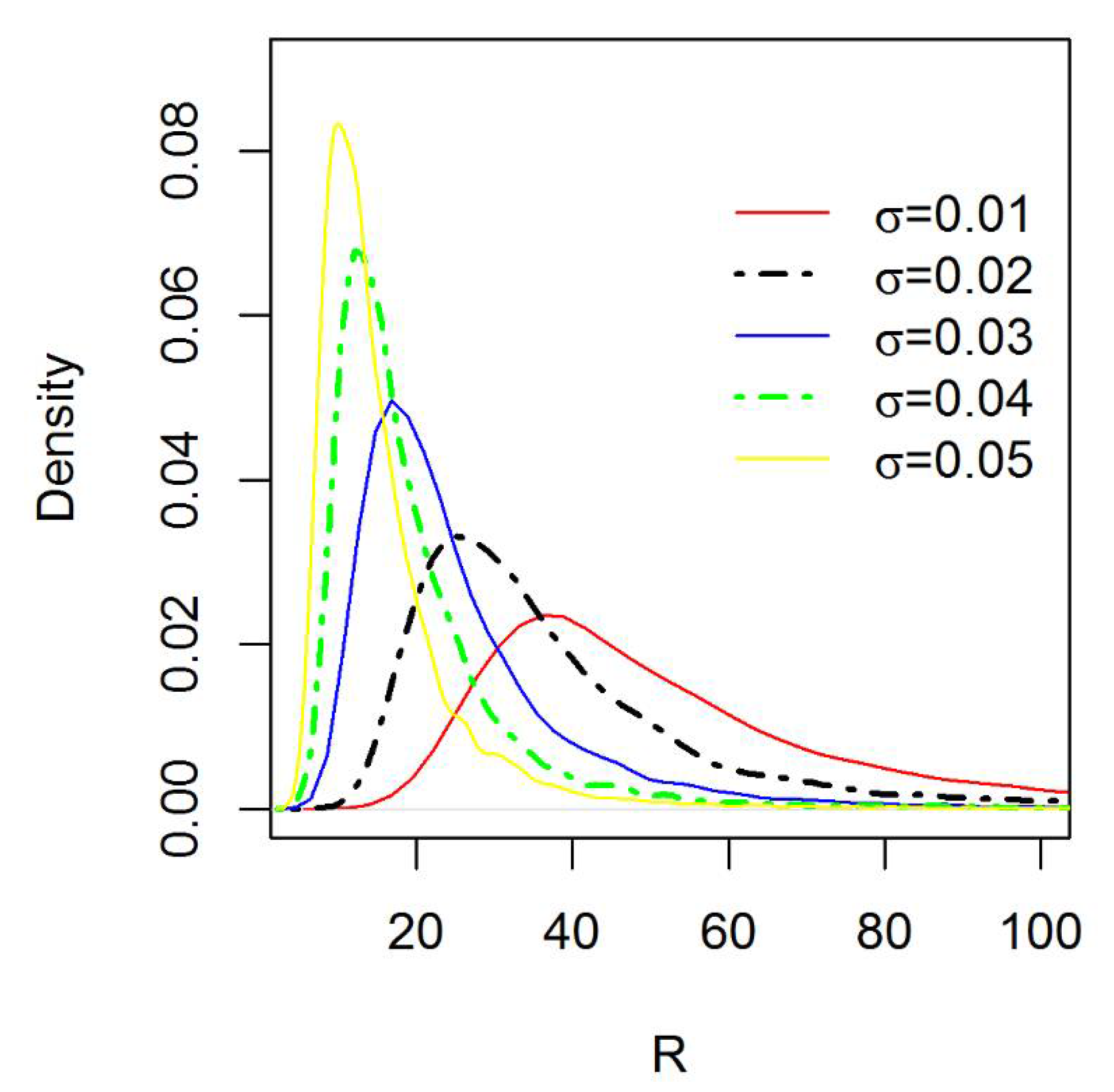
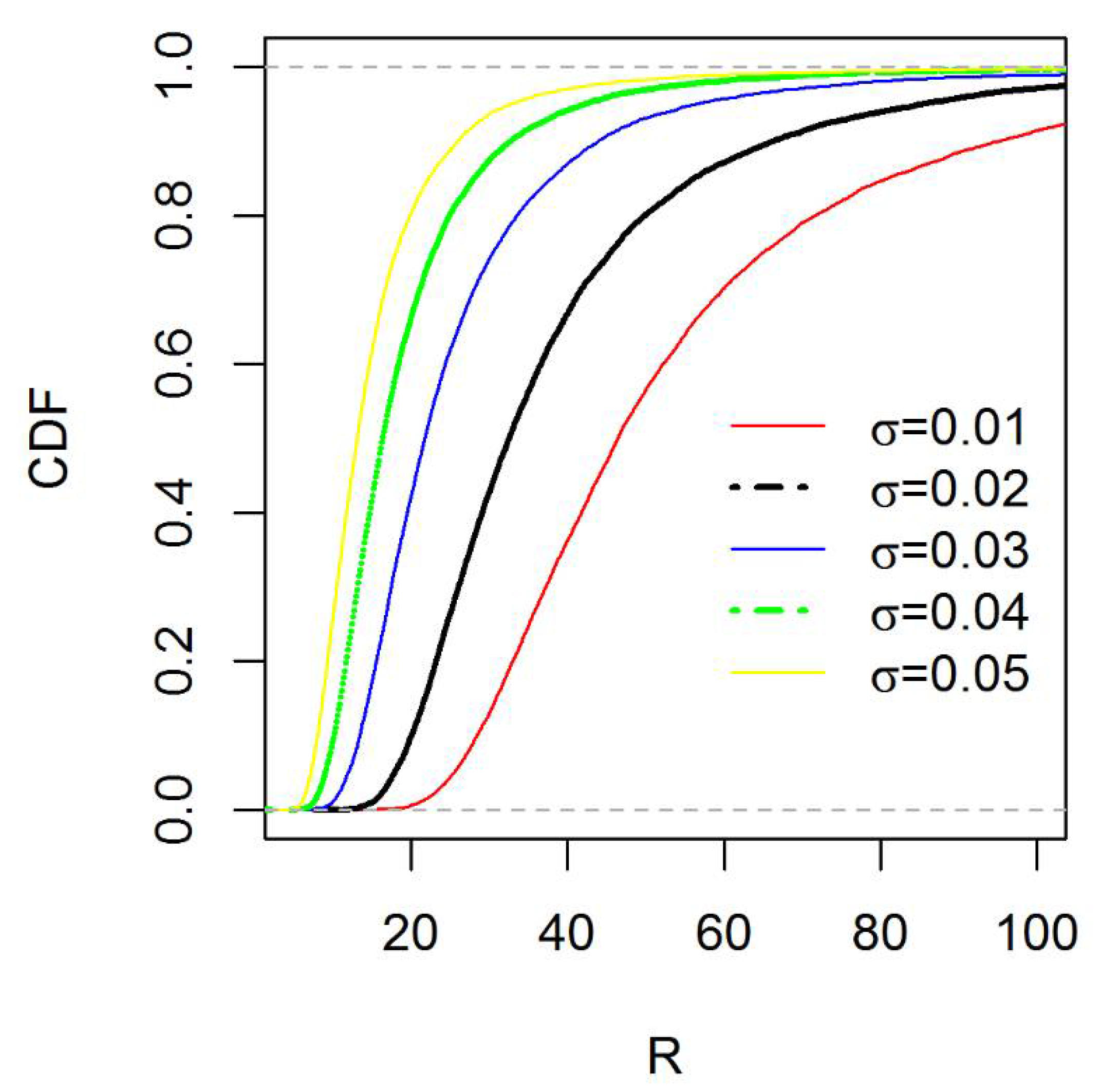
2.1. Inverse Maxwell Distribution and Its Properties

Assume a random variable $X$ is continuous and holds the assumptions of Maxwell distribution with a single scale parameter $\sigma$. According to this consideration, the probability density function (PDF) and cumulative distribution function (CDF) of Maxwell distribution can respectively be expressed as

$$f\left(x,\sigma \right)=\sqrt{\frac{2}{\pi }} {\sigma }^{-3}{x}^2{e}^{-x^2/2{\sigma }^2};x>0$$

(1)

$$\mathrm{and}F\left(x\right)=\frac{2}{\sqrt{\pi }} \gamma \left(\frac{3}{2},\frac{x^2}{2{\sigma }^2}\right),$$

(2)

where

$${\int }_0^u{x}^{v-1}{e}^{-\mu x}dx={\mu }^{-v}\gamma \left(v,\mu u\right).$$

(3)

As in [10], if we consider $R=X^{-1}$ where $X$ is a Maxwell random variable, then the generated random variable R can be declared as an inverse Maxwell random variable. By adopting inverse transformation, we can derive the PDF of this distribution from Maxwell distribution with scale parameter $\sigma$ as

$$f\left(r,\sigma \right)=\sqrt{\frac{2}{\pi }} {\sigma }^{-3}{r}^{-4}{e}^{-\frac{1}{2r^2{\sigma }^2}};r>0.$$

(4)

Note that [26] uses another version of the inverse Maxwell distribution. The version in [26] can be obtained from this version by applying the transformation $X=\frac{\sqrt{2}\sigma }{\sqrt{\theta }}R.$ From (4) above, the CDF of the inverse Maxwell distribution can be obtained as

$$F\left(r\right)=\frac{2}{\sqrt{\pi }}\left[1-\gamma \left(\frac{3}{2},\frac{1}{2r^2{\sigma }^2}\right)\right];r>0.$$

(5)

Note that the integration of Equation (4) over the entire range is one. That is, ${\int }_0^{\infty }f\left(r,\sigma \right)=1$. Since Equation (4) is simultaneously nonnegative valued, it is verified as a PDF. From Figure 1 and Figure 2, we can state that PDF and CDF of the inverse Maxwell distribution are, respectively, positively skewed and monotonically increasing.

Figure 1. The inverse Maxwell probability density functions (PDFs) for different parameter values.

Figure 2. The inverse Maxwell cumulative distribution functions (CDFs) for different parameter values.

From the literature, several properties of inverse Maxwell distribution have been studied, but some important properties like entropy and Fisher information have yet to be provided. Moreover, as can be found in later application sections of this paper, it is important to discuss raw moments, as they provide the basis for theoretical development of control charts. So, in Appendix A, these properties are provided.

2.2. Derivation of the $V_{IM}$ Control Chart

Shewhart control chart is one sophisticated tool to detect the variation of scale parameter $\sigma$in process monitoring. Although the Shewhart control chart is originally used to monitor normally distributed process, we propose a new control chart for evaluating non-normally distributed processes. In this study, the inverse Maxwell distribution is considered, and the suggested chart is $V_{IM}$ control chart. For this, we will introduce a pivotal quantity $Q$ and define an estimate of ${\sigma }^2$ named $V_{IM}$. The $V_{IM}$ control chart is developed under the probability limits and $L$-sigma limits. In case of probability limits, the lower probability limits and upper probability limits are denoted by LPL and UPL. Similarly for the second case, the lower control limit, the $centerline$ and the $uppercontrollimit$ are denoted by $LCL$, $CL,$ and $UCL$. To define $LPL$ and$UPL$ or $LCL\mathrm{and}UCL$, we need to estimate the $\alpha -th$quantile or mean and variance of $V_{IM},$ respectively. The procedure is described in the following paragraphs.

From the PDF that is given in Equation (4), we let, $p=\frac{1}{2r^2{\sigma }^2}$, and by simplification we get $r=\sqrt{\frac{1}{2{\sigma }^{2}p}}$. Then the Jacobian of transformation becomes $J=\frac{dr}{dp}=\frac{1}{2\sqrt{2}\sigma p^{\frac{3}{2}}}$. Now, the distribution of $P$ can be written as

$$f_P\left(p\right)=\frac{2}{\sqrt{\pi }}{p}^{\frac{1}{2}}{e}^{-p}.$$

Finally, we can write this in a more familiar form as follows:

$$f_P\left(p\right)=\frac{1}{\mathsf{\Gamma }\left(\frac{3}{2}\right)}{p}^{\frac{3}{2}-1}{e}^{-p}.$$

(6)

The above expressed equation is a gamma density where the shape and scale parameters are $3/2$ and $1,$ respectively. Symbolically, we can write ${\left(2R^2{\sigma }^2\right)}^{-1}~gamma\left(\frac{3}{2},1\right)$.

Now, according to the additive property of the gamma distribution, we can write the sum of independent and identically distributed function of inverse Maxwell variates, ${\sum }_{i=1}^n{P}_i~gamma\left(\frac{3n}{2},1\right)$. In addition, remember the MLE of scale parameter derived in Equation (A4) in Appendix A and let ${\widehat{\sigma }}^2=V_{IM}$. As ${\widehat{\sigma }}^2$ is estimated from the sample observations in different time points, the values of ${\widehat{\sigma }}^2$are not the same across time, it is thus as random variable. So, we can write $V_{IM}={\left(3n\right)}^{-1}{\sum }_{i=1}^n\frac{1}{r_i^2}$ $\Rightarrow \frac{3n{V}_{IM}}{2{\sigma }^2}={\sum }_{i=1}^n{P}_i.$

Finally, we can consider $Q$ as a pivotal quantity, and the PDF of $Q$ follows a gamma distribution with parameters $3n/2$ and $1$. Here,$Q$ is a gamma distributed random variable, so its mean is $E\left[Q\right]=E\left[\frac{3n{V}_{IM}}{2{\sigma }^2}\right]=\frac{3n}{2}.$ Thus, we can write$E\left[\frac{V_{IM}}{{\sigma }^2}\right]=1\Rightarrow E\left[V_{IM}\right]={\sigma }^2$. Therefore,

$$E\left[V_{IM}\right]={\sigma }^2.$$

(7)

Equation (7) states that $V_{IM}$ is an unbiased estimator of${\sigma }^2$. Following the above procedure, first we find the variance of $Q$, and from this we can calculate the variance of$V_{IM}$.

The variance of$Q$is $Var\left(Q\right)=Var\left[\frac{3n{V}_{IM}}{2{\sigma }^2}\right]=\frac{3n}{2}$. This means that $\left[\frac{3n}{2{\sigma }^4}\right]Var\left(V_{IM}\right)=1$. Hence,

$$Var\left(V_{IM}\right)=\frac{2{\sigma }^4}{3n}.$$

(8)

The CDF of the pivotal quantity,$Q$ follows gamma distribution with parameters $3n/2$ and$1$, i.e., $F\left(q\right)=\frac{1}{\mathsf{\Gamma }\left(\frac{3n}{2}\right)}\gamma \left(\frac{3n}{2},q\right)$, where $\gamma \left(.,.\right)$ denote the incomplete gamma function. So, the $\alpha -th$ quantile can be derived as

$$V_{I{M}_{\alpha }}=\left(\frac{2{\sigma }^2}{3n}\right)F^{-1}\left(\alpha \right).$$

(9)

Now, the probability limits for $V_{IM}$ can be written as

$$LPL:V_{I{M}_{\frac{\alpha }{2}}}=\left[\frac{2{\sigma }^2}{3n}\right]F^{-1}\left(\frac{\alpha }{2}\right),\mathrm{and}UPL:V_{I{M}_{1-\frac{\alpha }{2}}}=\left[\frac{2{\sigma }^2}{3n}\right]F^{-1}\left(1-\frac{\alpha }{2}\right).$$

These can also be presented as

$$LPL:V_{I{M}_{\frac{\alpha }{2}}}=L_1{\sigma }^2,\mathrm{and}UPL:V_{I{M}_{1-\frac{\alpha }{2}}}=L_2{\sigma }^2$$

where $L_1=\left[\frac{2}{3n}\right]F^{-1}\left(\frac{\alpha }{2}\right)$ and $L_2=\left[\frac{2}{3n}\right]F^{-1}\left(1-\frac{\alpha }{2}\right)$. In Table 1, we provide several estimated values of these coefficients from the gamma distribution for various combinations of false alarm rate $\alpha$ and sample size $n$.

Table 1. Gamma quantiles for various values of $n$ and $\alpha .$

Sample Size (n)	$\mathbf{False}\mathbf{Alarm}\mathbf{Rate}\mathit{\alpha }$
	0.005		0.0027		0.002
	${\mathit{L}}_1$	${\mathit{L}}_2$	${\mathit{L}}_1$	${\mathit{L}}_2$	${\mathit{L}}_1$	${\mathit{L}}_2$
1	0.0150	4.7734	0.0099	5.0294	0.0081	5.4221
2	0.0878	3.3749	0.0706	3.6228	0.0635	3.7430
3	0.1611	2.8292	0.1380	3.0101	0.1280	3.0975
4	0.2218	2.5265	0.1959	2.6722	0.1845	2.7425
5	0.2713	2.3300	0.2442	2.4536	0.2322	2.5132
6	0.3124	2.1901	0.2848	2.2987	0.2725	2.3507
7	0.3471	2.0845	0.3194	2.1819	0.3070	2.2284
8	0.3768	2.0014	0.3493	2.0901	0.3369	2.1324
9	0.4027	1.9338	0.3753	2.0156	0.3630	2.0546
10	0.4254	1.8777	0.3984	1.9538	0.3862	1.9901

In process monitoring, we usually face two situations, and these cases are when the desired parameter ${\sigma }^2$ is known or unknown. When dealing with known${\sigma }^2$, the limits will be defined as

$$LPL=L_1{\sigma }_0^2; CL={\sigma }_0^2 \mathrm{and}UPL=L_2{\sigma }_0^2.$$

(10)

We will estimate $V_{IM}$ when ${\sigma }^2$ is unknown and use the estimated value for evaluating the process

$$LPL=L_1{\overline{V}}_{IM}; CL={\overline{V}}_{IM} \mathrm{and}UPL=L_2{\overline{V}}_{IM}$$

(11)

where ${\overline{V}}_{IM}$ is the estimated value of $V_{IM}$ and is calculated from the estimates of $V_{IM}$ attained from each of the sample batches over time, and finally taking their average.

Adopting the two moments of $V_{IM}$ found in Equations (7) and (8), $L$-sigma limits of $V_{IM}$ are presented as

$$\begin{gathered} LCL=E\left[V_{IM}\right]-L\times SD\left(V_{IM}\right) \\ =\left[1-L\sqrt{\frac{2}{3n}}\right]{\sigma }^2=W_1{\sigma }^2, \end{gathered}$$

(12)

$$CL=E\left[V_{IM}\right]={\sigma }^2, \mathrm{and}$$

(13)

$$\begin{gathered} UCL=E\left[V_{IM}\right]+L\times SD\left(V_{IM}\right) \\ =\left[1+L\sqrt{\frac{2}{3n}}\right]{\sigma }^2=W_2{\sigma }^2, \end{gathered}$$

(14)

where $W_1=\left[1-L\sqrt{\frac{2}{3n}}\right]$ and $W_2=\left[1+L\sqrt{\frac{2}{3n}}\right]$. Table 2 below contains the values of the L coefficient calculated from the gamma quantiles by maintaining some desired false alarm rate $\left(\alpha \right)$.

Table 2. L coefficients.

Sample Size $\left(\mathit{n}\right)$	$\mathbf{False}\mathbf{Alarm}\mathbf{Rate}\left(\mathit{\alpha }\right)$
	0.005	0.0027	0.002
	$\mathit{L}$	$\mathit{L}$	$\mathit{L}$
2	0.3379	0.2706	0.2432
3	0.8675	0.7394	0.6851
4	1.5369	1.3517	1.2715
5	2.3004	2.0623	1.9579
6	3.1324	2.8450	2.7180
7	4.0168	3.6833	3.5351
8	4.9431	4.5661	4.3979
9	5.9038	5.4856	5.2984
10	6.8934	6.4360	6.2307

Similar to the probability limit approach, we also observe two circumstances: One when ${\sigma }^2$ is known and the other when ${\sigma }^2$ is unknown. When ${\sigma }^2$ is known, the limits can be expressed as

$$LCL=W_1{\sigma }_0^2, CL={\sigma }_0^2\mathrm{and} UCL=W_2{\sigma }_0^2.$$

When we don’t have any previous value of${\sigma }^2$, we will estimate $V_{IM}$ beforehand (typically in a phase I study) and use it as follows:

$$LCL=W_1{\overline{V}}_{IM}, CL={\overline{V}}_{IM}\mathrm{and}UCL=W_2{\overline{V}}_{IM}$$

Table 3 illustrates the different values of factors $W_1$ and$W_2$. These values are calculated by using L coefficients, which are expressed in Table 2. By using these values, we can easily develop a control chart for the inverse Maxwell parameter.

Table 3. Factors for developing a control chart for monitoring inverse Maxwell distributed processes.

Sample Size (n)	False Alarm Rate (α)
	0.005		0.0027		0.002
	W1	W2	W1	W2	W1	W2
2	0.8049	1.1951	0.8438	1.1562	0.8596	1.1404
3	0.5911	1.4089	0.6514	1.3486	0.6770	1.3229
4	0.3726	1.6274	0.4482	1.5518	0.4809	1.5191
5	0.1600	1.8400	0.2470	1.7531	0.2851	1.7149
6	0.0000	2.0441	0.0518	1.9483	0.0939	1.9060
7	0.0000	2.2396	0.0000	2.1367	0.0000	2.0909
8	0.0000	2.4270	0.0000	2.3181	0.0000	2.2696
9	0.0000	2.6068	0.0000	2.4930	0.0000	2.4420
10	0.0000	2.7799	0.0000	2.6618	0.0000	2.6087

The main purpose of constructing a control chart is to identify whether or not shift is available in a process. Therefore, we will test the following hypothesis.

Null hypothesis$H_0:{\sigma }^2={\sigma }_0^2;$or$\delta =1,$(i.e., no shift is available in the process)

versus

Alternative hypothesis$H_1:{\sigma }^2={\sigma }_1^2=\delta {\sigma }_0^2;$or$\delta \ne 1,$(i.e., shift is available in the process.)

Here, $\delta$ indicates that the shift is available in the process.

3. Results

This section presents the results of the performance of the proposed $V_{IM}$ control chart and discusses the results.

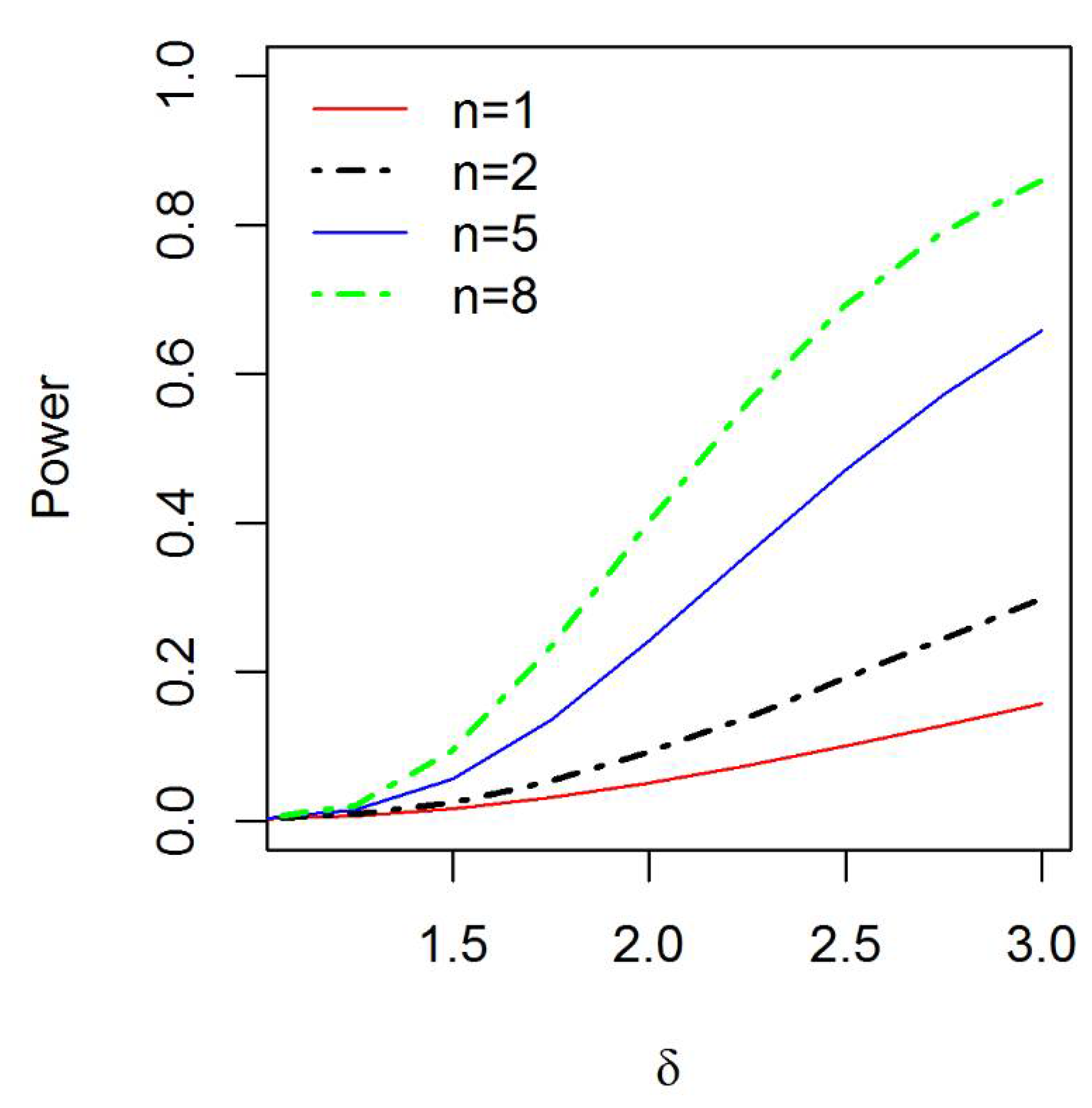
3.1. Performance Evaluation

Performance of control charts can be evaluated using various measures: Power curves, run length curves, or different run length summaries such as average run length (ARL), standard deviation of run length (SDRL), median run length (MDRL), and percentiles of run length. The performance of $V_{IM}$ control chart based on these tools is also provided in the paragraphs below.

The power of a test is defined by the probability of rejecting the null hypothesis$\left(H_0\right)$ when an alternative hypothesis$\left(H_1\right)$ is true. That is,$Power=Pr\left(reject H_0|H_1\right)$. In our study, power is the probability of correctly rejecting the null hypothesis when the value of the plotting statistic ($V_{IM}$) is either less than the lower probability limit or greater than the upper probability limit. Mathematically, it is expressed as

$$Power=Pr\left(V_{I{M}_{\alpha }}<LP{L}_0|H_1\right)+Pr\left(V_{I{M}_{\alpha }}>UP{L}_0|H_1\right)$$

which is equivalent to

$$Power=Pr\left(V_{I{M}_{\alpha }}<\left(\frac{2{\sigma }_0^2}{3n}\right)F^{-1}\left(\frac{\alpha }{2}\right)|\delta \ne 1\right)+Pr\left(V_{I{M}_{\alpha }}>\left(\frac{2{\sigma }_0^2}{3n}\right)F^{-1}\left(1-\frac{\alpha }{2}\right)|\delta \ne 1\right)$$

where $F^{-1}\left(\alpha \right)=\frac{3nV}{2{\sigma }^2}$. Therefore, power of the proposed $V_{IM}$ chart is derived as follows:

$$Power=1+\frac{1}{\mathsf{\Gamma }\left(\frac{3n}{2}\right)}\gamma \left(\frac{3n}{2},{\delta }^{-1}{F}^{-1}\left(\frac{\alpha }{2}\right)\right)-\frac{1}{\mathsf{\Gamma }\left(\frac{3n}{2}\right)}\gamma \left(\frac{3n}{2},{\delta }^{-1}{F}^{-1}\left(1-\frac{\alpha }{2}\right)\right).$$

(15)

If $\delta =1$, that is when the shift is totally absent from the process, then Equation (15) reduces to the false alarm rate$\alpha$. Figure 3 depicts the power for various process shift and sample sizes. When sample size increases, power also increases. So, from the figure, we can conclude that our proposed chart also works for larger shifts, and as the shift increases, the power also increases.

Figure 3. Power curves of $V_{IM}$ chart for various $n$ at $\alpha =0.0027$.

We can also use ARL (Average Run Length) to inspect the performance of the control chart. The traditional definition of ARL is

$$ARL=\frac{1}{1-\beta }=\frac{1}{power}.$$

(16)

For illustration, we have estimated the ARL by Equation (16) and by Monte Carlo simulations. The values of ARL are approximately similar for both procedures. Because of this, we only report the simulated result in Table 4 below. In Appendix B, the computational code used to estimate these values are provided. The $SDRL$ and $MDRL$ values that are generated by the Monte-Carlo simulation approach with 10,000 iterations are also given in the table. We use subgroup sizes of $n=1,3, 6, \mathrm{and} 10,$ and set the false alarm rate to $\alpha =0.0027$. The performance of the $V_{IM}$ chart is also investigated for various shift sizes of $\delta =1.00, 1.25, 1.50, 1.75, 2.00, 2.25, 2.50, 2.75, 3,$ and $5$.

Table 4. Average run length (ARL), standard deviation of run length (SDRL), and median run length (MDRL) of $V_{IM}$ chart for various $n$ at $\alpha =0.0027$.

$\mathbf{Sample}\mathbf{Size}\left(\mathit{n}\right)$
	1			3			6			10
$\mathit{\delta }$	ARL	$\mathit{S}\mathit{D}\mathit{R}\mathit{L}$	$\mathit{M}\mathit{D}\mathit{R}\mathit{L}$	$\mathit{A}\mathit{R}\mathit{L}$	$\mathit{S}\mathit{D}\mathit{R}\mathit{L}$	$\mathit{M}\mathit{D}\mathit{R}\mathit{L}$	$\mathit{A}\mathit{R}\mathit{L}$	$\mathit{S}\mathit{D}\mathit{R}\mathit{L}$	$\mathit{M}\mathit{D}\mathit{R}\mathit{L}$	$\mathit{A}\mathit{R}\mathit{L}$	$\mathit{S}\mathit{D}\mathit{R}\mathit{L}$	$\mathit{M}\mathit{D}\mathit{R}\mathit{L}$
1.00	370.14	371.53	258	370.55	369.10	258	369.29	368.13	257	369.85	369.25	254
1.25	146.15	145.07	101	96.07	93.96	67	60.40	60.34	42	39.37	39.16	27
1.50	62.37	61.33	44	28.76	28.25	20	14.47	14.01	10	8.16	7.70	6
1.75	32.32	31.69	23	12.73	12.13	9	6.04	5.52	4	3.31	2.69	2
2.00	19.95	19.29	14	7.37	6.79	5	3.36	2.83	2	2.02	1.45	1
2.25	13.44	13.01	9	4.71	4.12	3	2.33	1.77	2	1.48	0.84	1
2.50	9.96	9.41	7	3.47	2.94	3	1.82	1.23	1	1.26	0.58	1
2.75	7.80	7.23	6	2.77	2.17	2	1.52	0.90	1	1.14	0.39	1
3	6.39	5.99	5	2.31	1.72	2	1.35	0.68	1	1.08	0.29	1
5	2.70	2.15	2	1.26	0.57	1	1.03	0.17	1	1.00	0.02	1

In case of an out of control situation, smaller values of ARL than the in-control values of ARL are desired for any control chart. From Table 4, we observe the following results:

• The average run length (ARL) is always approximately 370 when the process is in control, (i.e., $\delta =1$) for all considered sample sizes.
• For an in-control process, there is no significant difference between the SDRL values and the corresponding ARL values for any sample size, $n$. For example: The ARL and SDRL values are 370.55 and 369.10, respectively, at $n=3$. Similarly, when $n=10$, the ARL and SDRL values are 369.85 and 369.25 respectively.
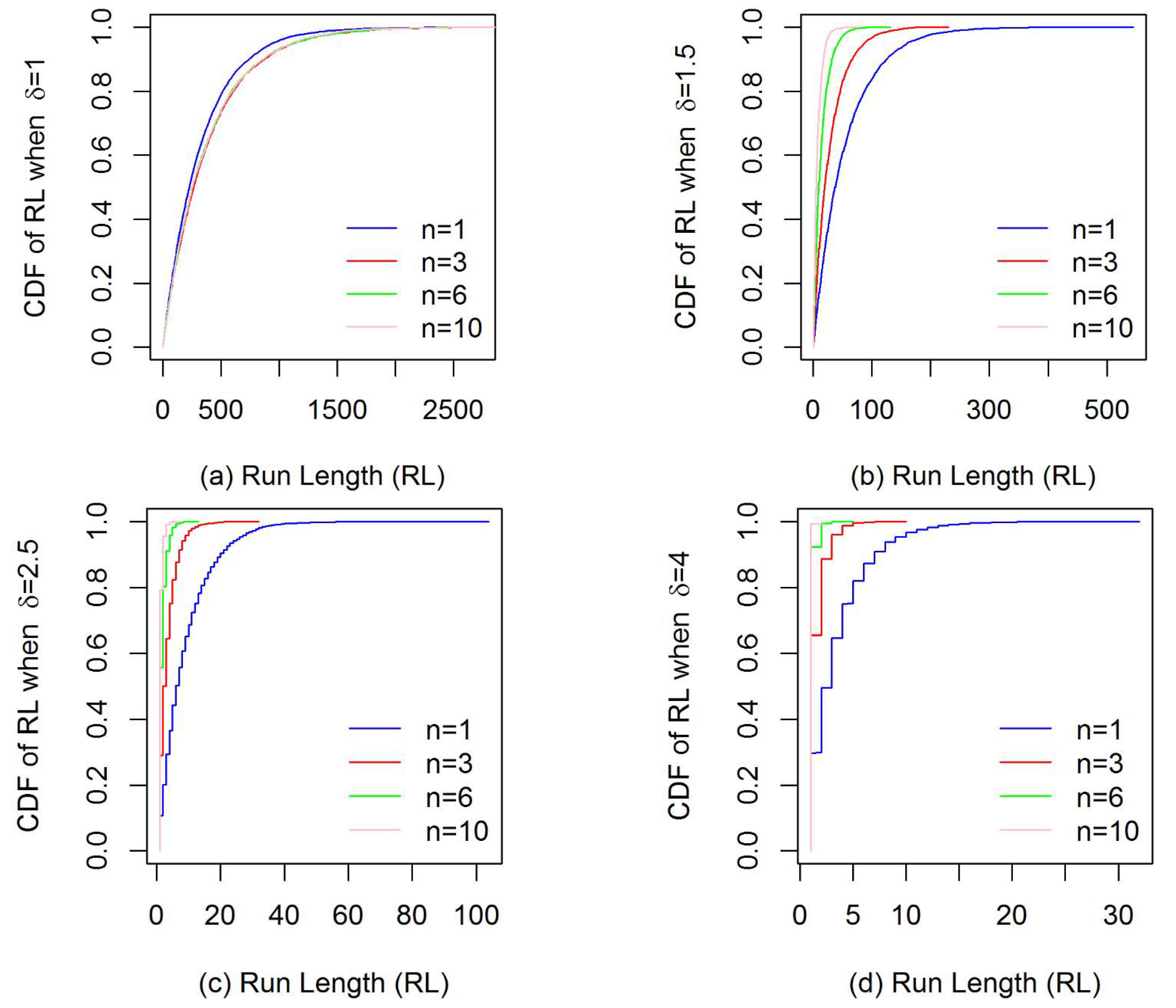
• The ARL and SDRL values rapidly decrease as the shift increases in the process scale parameter. For example: At 50% increment of shift and for $n=3,$ the ARL and SDRL are 28.76 and 28.25, respectively. Under the same condition and at 150% increment of shift, the ARL and SDRL respectively become 3.47 and 2.94. From these values, we can also conclude that the ARL and SDRL are directly proportional to each other.
• In both the in-control and out-of-control situations and for any sample size, the ARL values are greater than the MDRL values. This indicates that the run length distribution of the $V_{IM}$chart is positively skewed. For example: When $n=3$ and $\delta =1.75$, the ARL and MDRL values are 12.73 and 9, respectively. Additionally, for $n=6$ and $\delta =2$, the ARL and MDRL values are 3.36 and 2, correspondingly.

The various percentiles of $RL,$ obtained by simulation, are also presented in Table 5. The computational codes are available in Appendix B. To make easy comparisons, RL curves for the proposed chart have been plotted for various combinations of shifts and sample sizes in Figure 4. The curves show that the RL distribution of $V_{IM}$chart is positively skewed, which supports our above-mentioned analysis, and its CDF is monotonically increasing. It can be visualized from the figures that the curves are getting lower as shift increases. Based on all these tools, we can infer that our proposed chart is good enough to evaluate an inverse Maxwell distributed process.

Table 5. Percentiles of RL of $V_{IM}$ chart for various $n$ at α = 0.0027.

$\mathbf{Sample}\mathbf{Size}\left(\mathit{n}\right)$
	1					3					6					10
$\mathit{\delta }$	${\mathit{P}}_{10}$	${\mathit{P}}_{25}$	${\mathit{P}}_{50}$	${\mathit{P}}_{75}$	${\mathit{P}}_{95}$	${\mathit{P}}_{10}$	${\mathit{P}}_{25}$	${\mathit{P}}_{50}$	${\mathit{P}}_{75}$	${\mathit{P}}_{95}$	${\mathit{P}}_{10}$	${\mathit{P}}_{25}$	${\mathit{P}}_{50}$	${\mathit{P}}_{75}$	${\mathit{P}}_{95}$	${\mathit{P}}_{10}$	${\mathit{P}}_{25}$	${\mathit{P}}_{50}$	${\mathit{P}}_{75}$	${\mathit{P}}_{95}$
1.00	41	106	258	514	1089	41	107	258	513	855	39	105	257	517	841	39	106	254	514	853
1.25	17	42	101	202	433	11	28	67	134	221	7	18	42	84	138	4	12	27	54	91
1.50	7	19	44	86	184	4	9	20	39	65	2	4	10	20	33	1	3	6	11	18
1.75	4	10	23	44	95	2	4	9	17	28	1	2	4	8	13	1	1	2	4	7
2.00	2	6	14	28	58	1	2	5	10	16	1	1	2	4	7	1	1	1	3	4
2.25	2	4	9	18	39	1	2	3	6	10	1	1	2	3	5	1	1	1	2	3
2.50	2	3	7	14	29	1	1	3	5	7	1	1	1	2	3	1	1	1	1	2
2.75	1	3	6	11	23	1	1	2	4	6	1	1	1	2	3	1	1	1	1	2
3.00	1	2	5	8	18	1	1	2	3	5	1	1	1	2	2	1	1	1	1	1
5	1	1	2	3	7	1	1	1	1	2	1	1	1	1	1	1	1	1	1	1

Figure 4. RL curves for different shifts $\delta$ and sample size $n$. (a) when $\delta =1$; (b) when $\delta =1.5$; (c) when $\delta =2.5$; (d) when $\delta =4$.

3.2. Simulation Study

In a simulation study, we generate a sample of random data in such a way that imitates a real problem. Here, we generate data from inverse Maxwell distribution and the proposed charts by the following algorithm:

• Step 1: Fix the sample size $n$ for each random sample.
• Step 2: Generate a random sample of size $n,$ from$T~gamma \left(3/2,2{\sigma }_0^2\right)$.
• Step 3: By taking the square root of $T$, we will get a sample from Maxwell random variable $X$ of size $n$.
• Step 4: Obtain a sample from the inverse Maxwell random variable $R$ of size $n$ by setting $R=1/X$.
• Step 5: Estimate the plotting statistics $V_{IM}$.
• Step 6: Repeat the first five steps until the expected amount of sample subgroups are obtained.
• Step 7: Develop the control limits as proposed in the previous section.
• Step 8: Plot all the values of $V_{IM}$ statistics in contrast to the control limits.

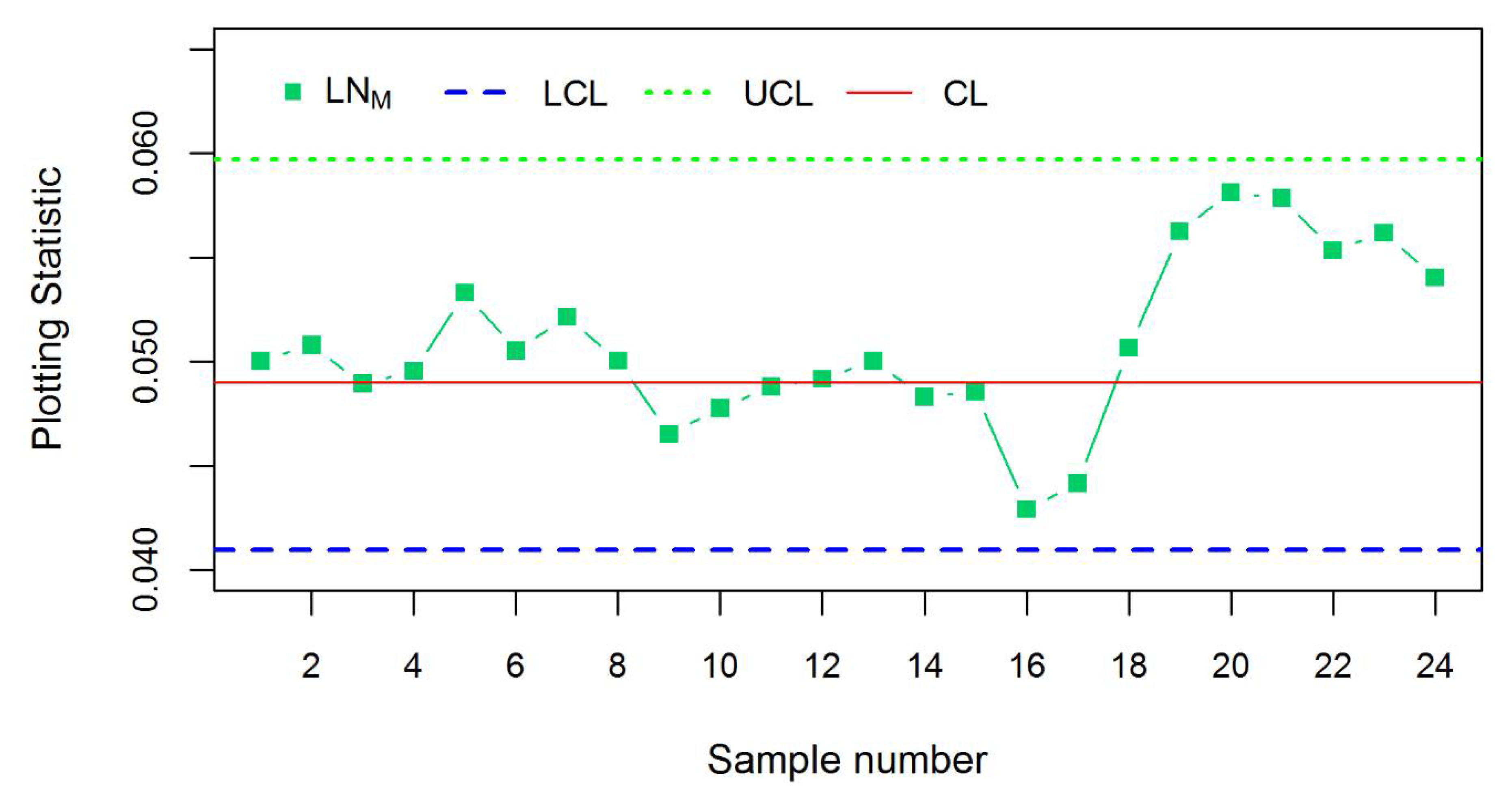
According to the above steps and by using statistical software $R \mathrm{3.4.2}$, we simulated data from inverse Maxwell distribution and cross checked the resulting data by Kolmogorov–Smirnov (K–S) test based on [27] to determine whether or not the data set follows the inverse Maxwell distribution. In this study, we assume ${\sigma }_0=100$ and generate 144 sample observations. By using the K–S test, we confirmed that the data follow the inverse Maxwell distribution. With this data confirmation, then we divide the data set into 24 samples each of size 6.

Then, from Table 1 for fixed false alarm rate$\alpha =0.0027$ and $n=6$, $L_1=0.2848$ and $L_2=2.2987$, and known ${\sigma }_0=100$, the resulting probability limits are

$$LPL=2848,CL=\mathrm{10,000}\mathrm{and}UPL=\mathrm{22,987}.$$

The visual representation of a $V_{IM}$ control chart according to these limits is provided in Figure 5.

Figure 5. $V_{IM}$-chart for inverse Maxwell parameter based on probability limits (In control and Out of control situations).

In case of $L$ sigma limit, we assume the same false alarm rate, sample size, and ${\sigma }_0$, the values of $W_1$ and $W_2$ are 0.0518 and 1.9483, respectively. So, the $L$ sigma limit becomes

$$LCL=518,CL=\mathrm{10,000}\mathrm{and}UCL=\mathrm{19,483}.$$

In Figure 5 and Figure 6, when the process has no shift, i.e., $\delta =1,$ no violations of the criteria given in [15] for out of control process can be seen. Therefore, we can state that the process is in control for both cases.

Figure 6. $V_{IM}$-chart for inverse Maxwell parameter based on $L$ sigma limits (In control and Out of control situations).

To inspect the ability of the chart for identifying out of control signals, we intentionally put a shift in the process scale parameter after the 18th sample in Figure 5 and Figure 6. So, the first 18 samples of the process remain in control where $\delta =1$ while the remaining samples contain a higher shift, that is $\delta =1.85$. According to the probability and $L$ sigma limits, we develop control charts for visualizing the out of control situation by adopting $\alpha =0.0027$, $n=6,$ and known ${\sigma }_0=100$. Figure 5 and Figure 6 demonstrate that both control charts detect two from six out of control signals.

In the literature, we learn that several leading control charts are typically applied to evaluate skewed process. To verify the necessity and suitability of $V_{IM}$ control chart, we monitor the data that have been generated from inverse Maxwell distribution by these leading Weibull, Gamma, and Lognormal control charts. That is, can inverse Maxwell process be adequately monitored by any of these leading charts? Ref. [28] proposed the construction procedure of these control charts by weighted variance (WV) and weighted standard deviation (WSD) method.

Figure 7 describes this control chart, where $W_M$ is the plotting statistics using the Weibull distribution. This $\overline{X}$ control chart for Weibull distribution suggest that the process is out of control because one point is out of the control limits, but the data is generated from an inverse Maxwell distribution in an in-control situation. So, we conclude that Shewhart control chart based on WV method for Weibull distribution is unable to adequately monitor an inverse Maxwell process. We also consider the Weibull and Gamma control charts under both the WV and WSD method, but do not furnish these in this paper to conserve space. Although both Weibull and Gamma distribution have scale and shape parameters and are thus theoretically more flexible than the inverse Maxwell that has only a scale parameter, we observe that the outcomes of Weibull and Gamma can be misleading.

Figure 7. $\overline{X}$ control chart under Weibull distribution for inverse Maxwell parameter using weighted variance method.

We can however monitor the inverse Maxwell process through the Lognormal based Shewhart control chart where this chart provides better results than the Weibull and Gamma control chart. The $\overline{X}$ control chart for Lognormal distribution under WV technique is able to monitor an inverse Maxwell process, but its shifts detection ability is worse compared to the proposed $V_{IM}$ control chart. Figure 8 shows that the Lognormal control chart can monitor an in-control inverse Maxwell process. Figure 9, however, shows that the process is still in-control even though the process actually contains 125% larger variations after the 18th sample. By comparing Figure 9 with Figure 5 and Figure 6, we can state that the $V_{IM}$ control chart monitors the inverse Maxwell process better than the existing Lognormal control chart.

Figure 8. $\overline{X}$ control chart under Lognormal distribution for inverse Maxwell parameter using weighted variance method.

Figure 9. $\overline{X}$ control chart under Lognormal distribution for inverse Maxwell parameter using weighted variance method ($125\%$after 18th sample).

3.3. Comparisons

In the previous section, we learned that the existing skewed distribution control charts are struggling to detect variations of an inverse Maxwell process, which underscores the necessity of $V_{IM}$ chart in SPC. However, that doesn’t make our proposed chart automatically superior than the existing charts. Moreover, can we infer that our newly proposed chart for monitoring a positively skewed process is more effective than the existing charts? As an answer to this question, and as a way to visualize the superiority of our proposed chart, the performance of our proposed chart is compared with the more recently improved Lognormal distributed control chart. Lognormal distributed control charts are widely used as candidate charts for evaluating positively skewed processes by several scholars. See for example [24,29,30,31], and so on. Lognormal S-chart is recently proposed by [24] for monitoring skewed process. They showed the suitability of this chart when the process standard deviation is high.

Since both charts deal with skewed processes, we compare the ARL of our proposed chart with the Lognormal S-chart to see whether our proposed chart is comparatively good or bad for monitoring skewed processes. Table 6 expresses this comparison, where the ARL of the Lognormal S-chart at $\sigma =1$ is taken from Table 9 of [24]. From Table 6, we see that for every out of control situation, the ARL values of the $V_{IM}$ control chart are less than the Lognormal S-chart. For example: At 50% increment of shift in the process, the number of samples of the Lognormal S-chart needed for shift detection is about 54 samples, whereas for this same quantity of shift, the number of samples is only about 18 in case of the $V_{IM}$ control chart. This shows the superiority of the inverse Maxwell control chart over the Lognormal S-chart. We also use several overall performance measures for better comparison. These include extra quadratic loss (EQL), performance comparison index (PCI), and Relative average run length (RARL), where smaller values indicate better performance quality. Based on [32]’s expressions for these performance measures, we observe that the EQL of our proposed chart is 48.73, while it is 126.71 is for the Lognormal S-chart. Similarly, the PCI and RARL of the Lognormal S-chart are 2.60 and 5.59, respectively, whereas under $V_{IM}$ chart both are equal to 1. Finally, we can conclude that the proposed chart is superior than the existing counterparts for monitoring a highly skewed process.

Table 6. ARL values of $V_{IM}$ and Lognormal S-charts for different shifts at $\sigma =1.00$and$n=5$.

$\mathbf{Shift}\left(\mathit{\delta }\right)$	Average Run Length
	${\mathit{V}}_{\mathit{I}\mathit{M}}\mathbf{Chart}$	Lognormal S-Chart
1	368.39	370.34
1.50	17.72	53.92
2.00	4.12	24.34
2.50	2.11	14.15
3.00	1.52	10.71
3.50	1.28	8.79
4.00	1.16	7.99

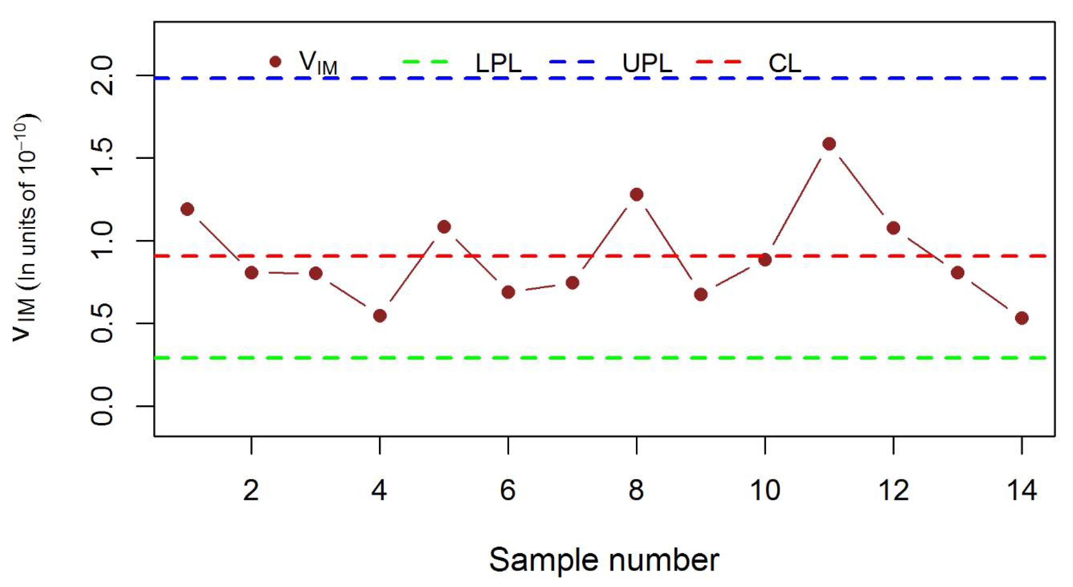
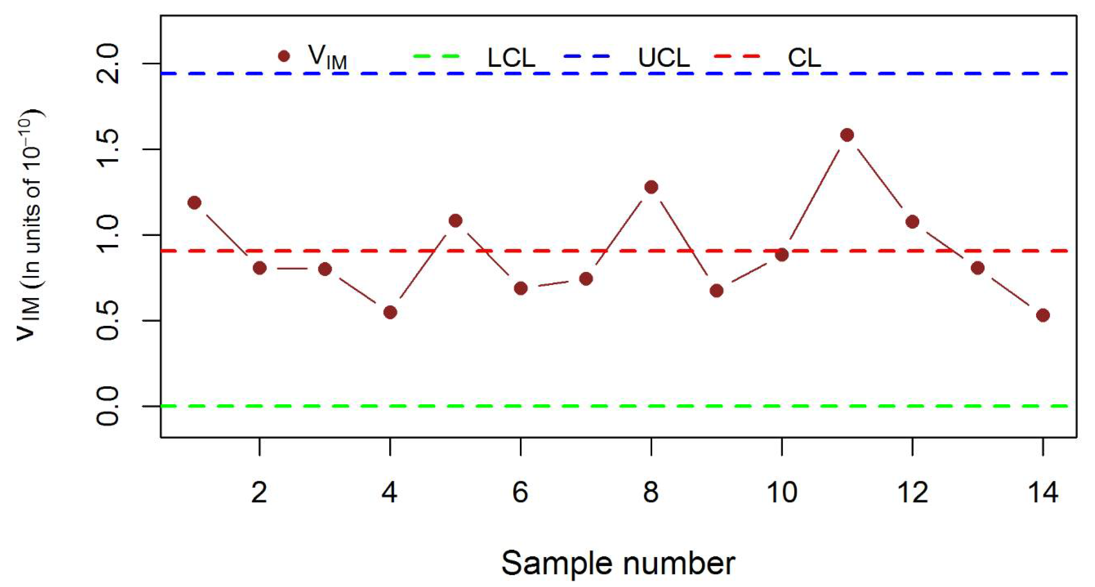
3.4. Real Life Example

Different kinds of data, such as lifetime data, time series data, and genetic data, may follow inverse Maxwell distribution. To highlight the pertinence of these control charts through a real-life example, we apply our proposed method to the car brake pedal lifetime data, which can be found in [33]. This data set is the left front brake pads’ lifetime on a sample of 98 vehicles and measured by the car odometer readings. The values reported in Table 7 represent measures of distance traveled by the selected vehicles before replacement of the initial brake pads. For example: The odometer reading of 22,200 km indicates that this particular vehicle covered a distance of 22,200 km before replacing its initial brake pads.

Table 7. Lifetime of car’s brake pad (in 1000 km).

Sample Number	Observations
	1st	2nd	3rd	4th	5th	6th	7th
1	22.2	23.0	24.0	28.6	21.8	17.0	26.0
2	23.2	18.9	21.9	27.3	13.8	24.0	20.1
3	15.7	26.8	27.9	15.3	28.8	16.0	23.6
4	53.8	21.7	28.8	17.0	16.5	15.7	28.0
5	13.3	16.5	24.2	17.6	27.8	18.3	17.7
6	20.0	13.2	16.9	14.9	15.5	7.0	15.8
7	15.0	38.3	11.2	38.2	26.7	17.1	29.0
8	18.3	18.4	18.2	15.9	16.4	23.6	19.2
9	23.3	20.4	20.9	28.5	23.2	17.9	46.1
10	39.3	11.8	17.7	30.9	22.4	45.0	18.2
11	30.2	21.8	18.2	23.0	27.2	10.9	25.5
12	12.4	39.9	17.7	26.3	14.1	21.0	11.2
13	10.8	25.7	32.4	13.6	19.1	16.1	53.3
14	57.3	36.5	19.7	20.8	30.8	20.0	39.6

To investigate whether or not the data set follows the inverse Maxwell distribution, we use the Kolmogorov–Smirnov (K–S) test. Here, we define the null hypothesis to be that the data set come from an inverse Maxwell distribution, while the alternative hypothesis is that the data set does not come from an inverse Maxwell distribution. For our car brake pads lifetime data set and under the above mentioned hypothesis, the K–S test statistic is 0.12 where the p-value is 0.452. Here, the K–S critical value of 0.14 for 5% level of significance is greater than the calculated statistic, and the level of significance is smaller compared to p-value. Therefore, we do not reject the null hypothesis and tend to entertain the idea that the inverse Maxwell distribution fits this data. From the simulation study, we learn that the existing control charts may not monitor the inverse Maxwell process well. However, the Maxwell V control chart could potentially be used. So, we further test whether or not the data set follows the Maxwell distribution according to the above testing procedure. If the data follows the Maxwell distribution, then we can instead apply the V control chart to monitor the cars’ brake pad lifetimes. However, the K–S test generates a p-value of 0.003 for our data set under the null hypothesis that the data follow Maxwell distribution. So, we reject the null hypothesis and infer that the data set does not follow the Maxwell distribution. This result verifies our earlier assessment that the inverse Maxwell distribution increases the application area of the Maxwell family of densities, and $V_{IM}$ chart is the better choice for monitoring an inverse Maxwell distributed process.

Thus, we adopt this brake pad data to develop the control chart for monitoring the inverse Maxwell parameter. The organization of the data set is presented in Table 7. The lifetime in 1000 km are as follows:

Now we form the proposed $V_{IM}$ control chart based on probability limits and $L$-sigma limits. From the data set, we get ${\overline{V}}_{IM}=9.08\times {10}^{-10}$ which is the estimated value of the MLE. We got L₁ = 0.3194 and L₂ = 2.1819 from Table 1 for $\alpha =0.0027$ and n = 7. Therefore, the probability limits become

$$LPL=2.90\times {10}^{-10},CL= 9.08\times {10}^{-10}\mathrm{and}UPL= 1.98\times {10}^{-9}.$$

In process control, several criteria are available for identifying the deficiencies of control charts including, among others, a point outside either the upper or lower control limit. Interested readers are referred to [15] for more details. None of the out of control criteria discussed by [15] are available in Figure 10. Therefore, we conclude that the process is in control.

Figure 10. $V_{IM}$-Chart for monitoring the inverse Maxwell parameter of the car brake pedal lifetime using probability limits.

Similarly, following [15], none of the out of control criteria are present in Figure 11. So, in this case, we can also state that there is no shift in the process.

Figure 11. $V_{IM}$-Chart for monitoring the inverse Maxwell parameter of the car brake pedal lifetime based on $L$-sigma limits.

Again, from Table 3 for fixed false alarm rate $\alpha =0.0027$ and n = 7, we have $W_1= 0$ and $W_2= 2.1367$. So, the probability limits become

$$LCL= 0,CL=9.08\times {10}^{-10}\mathrm{and}UCL=1.94\times {10}^{-9}.$$

4. Conclusions and Recommendations

Sometimes methods based on conventional distributions may not be adequate in real-life cases. Hence other alternatives are needed to enhance the application area. Partly due to this reason, several scholars have developed a variation of the Maxwell distribution called the inverse Maxwell distribution. In this demonstration, we study several important statistical properties of this distribution not yet recorded in the literature and provide an application of this distribution in Statistical Process Control.

In this article, we derive various properties of inverse Maxwell variables including the entropy, and the pdf of the sum, the difference, and the ratio of two independent variables. We also extend the properties to include a random sample of n variables so as to estimate the only parameter of the inverse Maxwell distribution using Maximum Likelihood Estimation (MLE). We also provide the Fisher information for the inverse Maxwell parameter. Some of these properties such as the pdf and the MLE are instrumental in establishing the design of the proposed control charts in this article.

We then show how to develop control charts for the inverse Maxwell parameter and provide several simulation results. Moreover, we compare the ability, efficiency, and superiority of the existing control charts especially under Weibull, Gamma, Lognormal and Maxwell distributions. We estimate several shift specific run length properties such as ARL, SDRL, and MDRL as well as overall variations identifying tools including EQL, RARL, and PCI of the proposed control chart for comparison. We observe that only Lognormal and Maxwell based control charts can potentially check an inverse Maxwell process, although their shift detection ability is far less than desired comparatively to the proposed control chart. Moreover, in special circumstances, the proposed $V_{IM}$ chart is more suitable than the existing Lognormal S-chart for identifying out of control signals in positively skewed process. Finally, a real-life example is provided which follow inverse Maxwell distribution where this control chart might be applicable to monitor the variability of an inverse Maxwell distributed process.

Recently, there are extensions of the Maxwell distributions such as the length-biased weighted Maxwell distribution discussed in [34] and more recently the Marshall–Olkin length-biased Maxwell distribution discussed in [35]. This study does not currently examine these extensions due to space limitations, but may consider these Maxwell extensions as possible interesting topics for future investigations in the same spirit as this paper.

References

- Sato, S.; Inoue, J. Inverse gaussian distribution and its application. Electron. Commun. Jpn. (Part III Fundam. Electron. Sci.) 1994, 77, 32–42. [Google Scholar] [CrossRef]
- Krishna, H.; Malik, M. Reliability estimation in Maxwell distribution with progressively Type-II censored data. J. Stat. Comput. Simul. 2012, 82, 623–641. [Google Scholar] [CrossRef]
- Tomer, S.K.; Panwar, M.S. Estimation procedures for Maxwell distribution under type-I progressive hybrid censoring scheme. J. Stat. Comput. Simul. 2015, 85, 339–356. [Google Scholar] [CrossRef]
- Brilliantov, N.V.; Pöschel, T. Deviation from Maxwell distribution in granular gases with constant restitution coefficient. Phys. Rev. E 2000, 61, 2809–2812. [Google Scholar] [CrossRef]
- Mohsin, S.; Kazmi, A.; Aslam, M.; Ali, S. On the Bayesian Estimation for two Component Mixture of Maxwell Distribution, Assuming Type I Censored Data. Int. J. Appl. Sci. Technol. 2012, 2, 197–218. Available online: http://www.ijastnet.com/journals/Vol_2_No_1_January_2012/23.pdf (accessed on 11 March 2020).
- Krishna, H.; Pundir, P. Discrete maxwell distribution. InterStat. J. 2007, 2007, 1–15. Available online: http://interstat.statjournals.net/YEAR/2007/articles/0711003.pdf (accessed on 2 January 2020).
- Mohsin, S.; Kazmi, A.; Aslam, M.; Ali, S. A Note on the Maximum Likelihood Estimators for the Mixture of Maxwell Distributions Using Type-I Censored Scheme. Open Stat. Probab. J. 2011, 3, 31–35. Available online: https://benthamopen.com/contents/pdf/TOSPJ/TOSPJ-3-31.pdf (accessed on 4 February 2020). [CrossRef]
- Hossain, M.P.; Omar, M.H.; Riaz, M. Estimation of mixture Maxwell parameters and its possible industrial application. Comput. Ind. Eng. 2017, 107, 264–275. [Google Scholar] [CrossRef]
- Karlis, D.; Santourian, A. Model-based clustering with non-elliptically contoured distributions. Stat. Comput. 2008, 19, 73–83. [Google Scholar] [CrossRef]
- Singh, K.L.; Srivastava, R.S. Inverse Maxwell Distribution as a Survival Model, Genesis and Parameter Estimation. Res. J. Math. Stat. Sci. 2014, 2, 23–28. [Google Scholar]
- Singh, K.L.; Srivastava, R.S. Estimation of the Parameter in the Size-Biased Inverse Maxwell Distribution. Int. J. Stat. Math. 2014, 10, 52–55. [Google Scholar]
- Singh, K.L.; Srivastava, R.S. Bayesian Estimation of Parameter of Inverse Maxwell Distribution via Size-Biased Sampling. Int. J. Sci. Res. 2014, 3, 1835–1839. [Google Scholar]
- Loganathan, A.; Chelvi, S.M.; Uma, M. Bayes Estimation of Parameter in Inverse Maxwell Distribution under Weighted Quadratic Loss Function. Int. J. Sci. Res. Math. Stat. Sci. 2017, 4, 13–16. [Google Scholar] [CrossRef]
- NIST/SEMATECH e-Handbook of Statistical Methods. Available online: https://www.itl.nist.gov/div898/handbook/ (accessed on 4 April 2020).
- Montgomery, D.C. Introduction to Statistical Quality Control, 6th ed.; John Wiley & Sons: Hoboken, NJ, USA, 2009. [Google Scholar]
- Woodall, W.H. Controversies and Contradictions in Statistical Process Control. J. Qual. Technol. 2000, 32, 341–350. [Google Scholar] [CrossRef]
- Roberts, S.W. Control Chart Tests Based on Geometric Moving Averages. Technometrics 1959, 1, 239–250. [Google Scholar] [CrossRef]
- Page, E.S. Continuous Inspection Schemes. Biometrika 1954, 41, 100–115. [Google Scholar] [CrossRef]
- Hossain, M.P.; Omar, M.H.; Riaz, M. New V control chart for the Maxwell distribution. J. Stat. Comput. Simul. 2017, 87, 594–606. [Google Scholar] [CrossRef]
- Hossain, M.P.; Sanusi, R.A.; Omar, M.H.; Riaz, M. On designing Maxwell CUSUM control chart: An efficient way to monitor failure rates in boring processes. Int. J. Adv. Manuf. Technol. 2018, 100, 1923–1930. [Google Scholar] [CrossRef]
- Zhang, C.W.; Xie, M.; Liu, J.Y.; Goh, T.N. A control chart for the Gamma distribution as a model of time between events. Int. J. Prod. Res. 2007, 45, 5649–5666. [Google Scholar] [CrossRef]
- Raza, M.; Raza, S.M.M.; Butt, M.M.; Siddiqi, A.F. Shewhart Control Charts for Rayleigh Distribution in the Presence of Type I Censored Data. J. ISOSS 2016, 2, 210–217. [Google Scholar]
- Raza, S.M.M.; Ali, S.; Butt, M.M. DEWMA control charts for censored data using Rayleigh lifetimes. Qual. Reliab. Eng. Int. 2018, 34, 1675–1684. [Google Scholar] [CrossRef]
- Huang, W.-H.; Yeh, A.B.; Wang, H. A control chart for the lognormal standard deviation. Qual. Technol. Quant. Manag. 2017, 15, 1–36. [Google Scholar] [CrossRef]
- Arafat, S.Y.; Hossain, M.P.; Ajadi, J.O.; Riaz, M. On the Development of EWMA Control Chart for Inverse Maxwell Distribution. J. Test. Eval. 2019, 49. [Google Scholar] [CrossRef]
- Tomer, S.K.; Panwar, M.S. A Review on Inverse Maxwell Distribution with Its Statistical Properties and Applications. J. Stat. Theory Pr. 2020, 14, 1–25. [Google Scholar] [CrossRef]
- Klugman, S.A.; Panjer, H.H.; Willmot, G.E. Loss Models from Data to Decisions, 4th ed.; John Wiley & Sons: Hoboken, NJ, USA, 2012. [Google Scholar]
- Derya, K.O.; Canan, H. Control charts for skewed distributions: Weibull, gamma, and lognormal. Metod. Zv. 2012, 9, 95–106. [Google Scholar]
- Chami, P.; Antoine, R.; Sahai, A. On Efficient Confidence Intervals for the Log-Normal Mean. J. Appl. Sci. 2007, 7, 1790–1794. [Google Scholar] [CrossRef][Green Version]
- Huang, W.-H.; Wang, H.; Yeh, A.B. Control Charts for the Lognormal Mean. Qual. Reliab. Eng. Int. 2015, 32, 1407–1416. [Google Scholar] [CrossRef]
- Joffe, A.D.; Sichel, H.S. A Chart for Sequentially Testing Observed Arithmetic Means from Lognormal Populations against a Given Standard. Technometrics 1968, 1, 605–612. [Google Scholar] [CrossRef]
- Abbasi, S.A.; Riaz, M.; Miller, A.; Ahmad, S.; Nazir, H.Z. EWMA Dispersion Control Charts for Normal and Non-normal Processes. Qual. Reliab. Eng. Int. 2015, 31, 1691–1704. [Google Scholar] [CrossRef]
- Lawless, J.F. Statistical Models and Methods for Lifetime Data; Wiley-Interscience: Hoboken, NJ, USA, 2002. [Google Scholar]
- Modi, K.; Gill, V. Length-biased Weighted Maxwell Distribution. Pak. J. Stat. Oper. Res. 2015, 11, 465. [Google Scholar] [CrossRef][Green Version]
- Mathew, J.; Chesneau, C. Marshall–Olkin Length-Biased Maxwell Distribution and Its Applications. Math. Comput. Appl. 2020, 25, 65. [Google Scholar] [CrossRef]
Publisher’s Note: MDPI stays neutral with regard to jurisdictional claims in published maps and institutional affiliations. |
© 2021 by the authors. Licensee MDPI, Basel, Switzerland. This article is an open access article distributed under the terms and conditions of the Creative Commons Attribution (CC BY) license (http://creativecommons.org/licenses/by/4.0/).