Abstract
Automatic segmentation of intracranial brain tumors in three-dimensional (3D) image series is critical in screening and diagnosing related diseases. However, there are various challenges in intracranial brain tumor images: (1) Multiple brain tumor categories hold particular pathological features. (2) It is a thorny issue to locate and discern brain tumors from other non-brain regions due to their complicated structure. (3) Traditional segmentation requires a noticeable difference in the brightness of the interest target relative to the background. (4) Brain tumor magnetic resonance images (MRI) have blurred boundaries, similar gray values, and low image contrast. (5) Image information details would be dropped while suppressing noise. Existing methods and algorithms do not perform satisfactorily in overcoming these obstacles mentioned above. Most of them share an inadequate accuracy in brain tumor segmentation. Considering that the image segmentation task is a symmetric process in which downsampling and upsampling are performed sequentially, this paper proposes a segmentation algorithm based on U-Net++, aiming to address the aforementioned problems. This paper uses the BraTS 2018 dataset, which contains MR images of 245 patients. We suggest the generative mask sub-network, which can generate feature maps. This paper also uses the BiCubic interpolation method for upsampling to obtain segmentation results different from U-Net++. Subsequently, pixel-weighted fusion is adopted to fuse the two segmentation results, thereby, improving the robustness and segmentation performance of the model. At the same time, we propose an auto pruning mechanism in terms of the architectural features of U-Net++ itself. This mechanism deactivates the sub-network by zeroing the input. It also automatically prunes GenU-Net++ during the inference process, increasing the inference speed and improving the network performance by preventing overfitting. Our algorithm’s PA, MIoU, P, and R are tested on the validation dataset, reaching 0.9737, 0.9745, 0.9646, and 0.9527, respectively. The experimental results demonstrate that the proposed model outperformed the contrast models. Additionally, we encapsulate the model and develop a corresponding application based on the MacOS platform to make the model further applicable.
1. Introduction
The brain is the most vital and complex organ in the human body, consisting of billions of cells [1], dominating all activity processes in the organism and regulating the balance between the organism and the surrounding environment. The brain tumor is a kind of neoplasm that grows in the brain with a high fatality rate. Brain tumors take up most of the intracranial space; they bring pressure to the brain tissues, affect the brain’s functionalities, severely damage patients’ central nerves, and destroy healthy brain cells. The components of the brain tumors are complex and can be primarily divided into different sub-areas, including the edema area, the enhanced tumor area, the non-enhanced tumor area, and the necrotic area [2]. At the same time, brain tumor categories are multiple and characteristic. Some tumors are troublesome to dissect, such as schwannoma [3], while there are impediments in locating some other tumors, such as glioma and glioblastoma [4].
Before performing an operation or radiotherapy and chemotherapy, doctors need to determine the tumor location as part of the general therapy. After confirming the location, doctors can obtain the tumor’s basic information, such as the shape, position, and size of tumors in different areas, and then design a more appropriate and accurate surgery and treatment strategy. Medical imaging techniques are adopted to detect and display the brain tumors to conduct the above-mentioned further treatment.
Current medical imaging techniques for brain tumors include PET-CT and MRI. MRI can reflect the anatomical structure of the human soft tissues, which has already become the preferred medical imaging method of brain diagnoses [5]. Radiology doctors can visually observe and define the range of the tumors according to the brain images manually. Typically, the characteristics they judge are the size, location, physiological traits, and metabolic condition.
However, there are various barriers to brain tumor segmentation with MRI.
- Brain tumor MR images exhibit intricate tumor structure and blurred boundaries, and external factors, such as noise, exist [6]. These factors make it difficult to determine the brain tumor scope.
- The gray values of different brain tissues are similar. The image contrast is low, and the noise and intensity of the scan are not uniform, which will lead to the lack of image information [7]. In such cases, doctors’ observations will be limited.
- There is high diversity in the appearance of tumor tissues, and similarity can be seen between tumor tissues and normal tissues, easily causing misdiagnosis and missed diagnoses [8].
- Traditional segmentation demands a discernible difference in the brightness of the object compared to the background. Image information details would be decreased while eliminating noise.
Until now, clinicians have relied on manual segmentation of the brain tumors in many cases [9], which requires doctors to have rich prior knowledge. Although some computer-assisted semi-automatic segmentation methods exist, many are complicated to operate and difficult to apply in clinical diagnosis. Therefore, as depicted above, brain tumors terribly impair human health. Moreover, the segmentation and classification of brain tumors are complicated due to their particular structure and character. Considering the clinic requirement and the medical value, developing an accurate, reliable, and fully automatic brain tumor segmentation algorithm has solid and crucial clinical significance [10].
The application of computer-aided systems has become one of the most active fields of study in the health industry. It has already been greatly developed, used in computational biomedical fields, and has made tremendous contributions [11]. Automatic segmentation based on deep-learning methods has recently become popular, among which, U-net is one of the most renowned frameworks for CNN. Through automatic segmentation, image features can be automatically learned [12]. At present, many new convolutional neural network design methods are based on the core idea of U-Net, and new modules for innovation and improvement are incorporated.
Thorsten Falk et al., for example, published an ImageJ plugin that analyzes data with U-Net, which includes pre-trained models for single-cell segmentation and enables U-Net to be tailored to new tasks using a few annotated samples [13]. In addition, Anita Khanna et al. proposed a type of deep residual U-Net CNN for automated lung segmentation, which can capture more distinguishing features instead of handcrafted ones, achieving 98.63%, 99.62%, and 98.68% accuracies for the LUNA16, VESSEL12, and HUG-ILD datasets, respectively. [14]. S Ghoshet proposed an improved U-Net with VGG-16 to segment Brain MR images and identify region-of-interest (tumor cells). The new U-Net achieved pixel accuracies of 0.994 and 0.9975 and was compared with the basic U-Net and improved U-Net architectures. It can be seen that the results surpassed traditional CNN-based state-of-the-art works [15].
In the field of brain tumor image segmentation, many experts continued proposing novel algorithms that optimized the preprocessing, segmentizing and classifying to improve the accuracy of the segmentation and classification for the brain tumor images. XZ A and other scientists proposed an efficient 3D residual neural network (ERV-Net) for brain tumor segmentation. The experimental results on the dataset of multimodal brain tumor segmentation challenge 2018 demonstrated that ERV-Net achieved the best performance with Dice of 81.8%, 91.21%, and 86.62% [16].
Li Sun et al. [17] suggested a deep learning-based framework for brain tumor segmentation and survival prediction in glioma using multimodal MRI data. They employed three different 3D CNN architectures ensembles to segment tumors for robust performance using a majority rule, reaching an excellent 61.0% accuracy on diverse levels of survivor classifications. S. Poornachandra et al. [18] used a CNN architecture to segment and preprocess by correcting MR image inhomogeneity, balancing histogram, and applying the Z-score normalization to all volumes. The Dice similarity coefficient it brings out is 0.68.
Shengcong Chen et al. [19] presented a Multi-Level DeepMedic for more accurate segmentation. They also proposed a novel dual-force training scheme to enhance the quality of multi-level learning features. In addition, they designed a label-distribution-based loss function to learn more abstract information. Salma Alqazzazl et al. [20] applied a fully convolutional neural network SegNet to 3D data sets for four MRI modalities for automated segmentation of brain tumor and achieved F-measure scores of 0.8, 0.81, and 0.79 for the whole tumor, tumor core, and enhancing tumor, respectively.
P. Ramya et al. [21] used several methods about ensemble clustering labels as the segmentation result. They also used the deep super-learning method to classify the anomalies. For the BraTS brain images dataset, the average accuracy rate reached 97%. Z Huang et al. [22] proposed a computer-aided brain tumor segmentation system based on an adaptive gamma correction neural network (GammaNet). Through the experiment, the Dice similarity coefficient (DSC), sensitivity, and intersection of union (IoU) of GammaNet were found to be 85.8%, 87.8%, and 80.31%.
Inspired by the above research status and previous studies, this paper proposes a segmentation algorithm based on U-Net++, consisting of a generative mask sub-network and an auto pruning mechanism, aiming to address problems and optimize solutions in the relative study field. The primary contributions of this paper are reflected as follows:
- Network structure based on MR image features. The basic model of 3D U-Net++ is adopted in this project to extract 3D features from 3D MR images. U-Net structures of different scales are fused into a neural network to strengthen the extraction of 3D features. In contrast, traditional networks merely obtain features from 2D images, which may share an extreme similarity between two adjacent 2D images and are not good enough for data feature extraction.
- Add generative mask sub-network to address overfitting in complex network structures. The model adds a generative mask sub-network branch to obtain a result of antagonistic generation, reducing the possibility of overfitting. The branch computes feature conditional probability distributions by extracting and simulating features in the highest dimension. The effect of segmenting the same sort of tumors outperforms the decision model. The result is combined with that generated by the upper part of the decision model. Then, calculate the loss to realize the sub-network regularization and reduce the error of the overall model.
- Two distinct training modes are under the same model. The pruning strategy of U-net++ is used to determine whether pruning should be carried out according to the given conditions during training. The input of the sub-network is set to zero to achieve structural inactivation, which could significantly improve the training speed and even reduce the over-fitting of the neural network, leading to the “dual-use of one model”.
The rest of this paper is divided into five parts: the Materials and Methods section introduces the dataset and design details of the generative mask sub-network; the Experiment section shows the experimental process and platform; the Results section shows the experimental results as well as their analysis; the Discussion section conducts numerous ablation experiments to verify the effectiveness of the optimized method and the limitation of our methods; and the Conclusion section summarizes the paper.
2. Materials and Methods
The dataset used in this paper is from BraTS 2018 [23], containing 285 cases in total. Each case has four modes: T1, T2, Flair, T1ce, and five labels: 0, 1, 2, 3, and 4. Precisely, label 0 corresponds to areas other than the domain with tumor, also known as background area. Label 1 represents the necrotic area of the tumor. Label 2 denotes the cyst region of the tumor. Label 3 corresponds to the non-enhanced region of the tumor. Label 4 corresponds to the enhanced area of the tumor, in which an MR sequence contains 155 images, each with a size of 240 × 240 pixels. Figure 1 is a case of a sequence in the BraTS dataset.
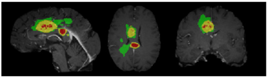
Figure 1.
Dataset samples.
A case has various sequences; each sequence consists of several slices, aiming to segment three components: whole tumor (WT), enhanced tumor (ET), and tumor core (TC). However, a single-mode often leads to failure or deficiency in the segmentation process due to insufficient subdivision of the tumor in the relevant area. Therefore, different MRI models are used to compensate for such weaknesses. Multiple image information modes can mutually complement, effectively developing segmentation accuracy. Nevertheless, although the input of image information from multiple modes increases the necessary information for segmentation, on the other hand, it also makes segmentation tricky by adding a large amount of unnecessary information.
2.1. Dataset Analysis
The BraTS training set is further divided into high-grade glioma (HGG) and low-grade glioma (LGG). HGG is a poorly differentiated glioma, which is malignant. Moreover, the patient’s prognosis is generally bleak. LGG is a well-differentiated glioma. Although this type of tumor is not biologically benign, the patient prognosis is relatively good.
Domain shift is a common problem in biomedical image analysis. Different institutions use different acquisition parameters to capture data for the first domain shift, resulting in the acquired images belonging to distinct domains. In this paper, the applied data set is from different MRI scanners of various medical institutions. Regarding the second type of domain shift, considering that the distribution of tumors and cancers may differ by grade and severity, training with HGG and LGG constrains the learning ability of segmentation models.
2.2. Data Enhancement
Medical image datasets carry fewer samples that need data enhancement to grow the amount and complexity of training samples. The following data enhancement methods are used in this paper to optimize insufficient network training caused via an insufficient data set or performance degradation caused by overfitting.
2.2.1. Basic Enhancement
This paper refers to the method proposed by Alex et al. [24]. Image flipping, image translation, image scaling, and noise adding are used to enhance the data. Flipping and translation are mainly used to improve model accuracy by increasing the amount of data, while scaling and noise adding are used to learn high-dimensional features by the low-frequency network. We use affine transformation to achieve the scaling of images.
It is assumed that the target image’s width and height are and , and the original image’s width and height are and . In this paper, is first calculated when the image is magnified and shrunk, as shown in Formula (1). After that, we divide the width and height of the original image by , and then take the part inside the target frame after the center point of the target frame is overlapped with the center point of the processed image. The section on noise addition is expanded in Section 2.2.2, comprising of methods, such as Cutout and CutMix.
2.2.2. Advanced Enhancement
In order to solve the enormous memory loss and the network’s unsatisfactory sensitivity to adversarial examples, we refer to the method depicted in the Mixup [25] and propose a 3DMix data enhancement method for 3D images. Since the generative mask sub-network is included in this model, enhancing the sensitivity of antagonistic samples can improve the accuracy of the generative sub-network, thus, improving the regularization effect of the final generated image. The method is shown in the Formulas (2)–(4).
is a batch sample, and is the label matching to the batch sample. is another batch sample, is the label matching to this batch sample, and is the mixing coefficient computed using the distribution of parameters and . When this method is implemented in this paper, there is no restriction on and . When the batch size is set to 1, two images are mixed.
When the batch size is greater than 1, it means that two Batch image samples are mixed accordingly. In addition, and can be either the same batch of samples or different batches of samples. When the method is implemented, and adopt the same batch of samples. Among them, is the original Batch image sample, and is obtained after shuffle processing of in the dimension of Batch size.
In addition, to prevent network overfitting, we use the dropout function proposed by Alex [24]. We perform a random erase operation on image data before data is inputted to the backbone network. The role of the Dropout function is similar to that of the dropout function [24]. As the part and area erased in each round of training are random, the robustness of the network can be enhanced, and the erased part will be regarded as the blocked or blurred part. There are two ways to deal with the erased part: filling pixels with a fixed color, such as black; filling with the RGB channel average of all pixels in the erased portion.
In addition to the above two methods, we also use Cutout [26] and CutMix [27] to process images.
Cutout takes a sample section at random and fills it with a specific pixel, leaving the classification result unaffected. The cutout is achieved by masking the image with a defined-size rectangle and then setting other solid colors within the rectangle or assigning all values to zero. Cutout allows CNN to employ global information from the entire image rather than local information from a few minor features.
The CutMix method is adopted to remove a portion of the region. The other data in the training set’s area pixel values are stochastically filled rather than filling zero pixels. CutMix allows the model to recognize two targets from a local view of an image, increasing the training efficiency. It also allows the model to focus on the areas where the target is hard to differentiate. However, there is a lack of knowledge in several areas, which will impact the training efficiency.
These specific effects are shown in Figure 2.
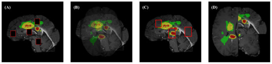
Figure 2.
Illustration of four augmentation methods. (A) Cutout; (B) MixUp; (C) CutMix; and (D) Mosaic.
2.3. GenU-Net++
U-Net++ [28], which has a U-shaped structure with a jump connection, is ideal for medical images segmentation. The network skeleton in this paper is U-Net++. Figure 3 depicts the network architecture of this paper. In order to improve the accuracy and prevent the gradient disappearance of data less than 0 in the convolution layer, we changed the activation function ReLU [29] of each block in the original model into LeakyReLU. We added a generative mask sub-network in the fifth layer of U-NET++. On the one hand, the generated mask feature maps will operate concatenation with the feature maps generated in the fifth layer and then be transmitted to the subsequent parts of u-Net.
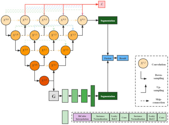
Figure 3.
Flow chart of GenU-Net++.
On the other hand, up-sampling will be carried out in the sub-network and predicted segmentation is generated. The Predicted segmentation generated by U-Net itself and the predicted segmentation generated by the sub-network will be fused in the Pixel Fusion Module. In the generative mask sub-network, we attempted three generative models: DCGAN [30], CVAE [31], and DCGAN-VAE [32], and the Instance Normalization layer replaces the Batch Normalization layer.
In addition, the deconvolution up-sample method commonly used in CNNs is replaced by the BiCubic interpolation algorithm. The experimental verification shows that the model performance obtained by this interpolation algorithm is superior to the deconvolution up-sampling method. In the weighted pixel fusion module, we reference the ideas of the NMS algorithm [33] and WBF algorithm [34] used in the target detection problem.
We give different weights to each pixel in the two predicted segmentation generated by U-Net [35] and generative mask sub-network, and the probability of the category to which each pixel belongs is obtained through a weighting operation. In this way, the prediction results of the two networks are fused, as shown in Algorithm 1.
| Algorithm 1 GenU-Net++ algorithm |
|
2.3.1. Generative Mask Sub-Network
In the generative mask sub-network, we first generate mask maps with the same dimension as feature maps of the U-Net++ fifth layer network based on Gaussian distribution. Then, the generated mask maps are concatenated with feature maps of the fifth layer of the network, and the effect is similar to that of the attention mechanism in SENet [36]. The masks generated by the generative model are used here to enhance features. At the same time, we carry out convolution and upsampling operations in the sub-network with mask maps and obtain the segmentation different from that of U-Net++. The specific structure of the generative mask sub-network is demonstrated in Figure 3.
The generator is employed to generate more available eigenvectors corresponding to lesion images to improve the training process. Consider DCGAN, which has two participants: the generator G and the discriminator D. Let be the distribution of retrieved eigenvectors. The generator model G’s purpose is to construct a probability distribution on the feature map x. This probability distribution is the estimated value of . Two deep neural networks represent the generator and discriminator. The DCGAN model’s optimization goal can be expressed mathematically as:
x is the prior value of the input noise variable in Formula (5). Two deep neural network models are trained during the training procedure. The generative model G is matched against the discriminative model. That is to say, through playing games, these two models will optimize their objective functions. Nevertheless, to avoid the difficulty of determining the exact Nash balance in the actual scenarios, the accuracy of the data generated in discriminator D is employed as a stopping requirement. This indicates that the training will be terminated if the misclassified probability of the data generated by G exceeds a predefined threshold. The training procedure is depicted in Figure 4.
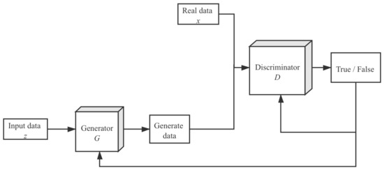
Figure 4.
Flow chart of the generative adversarial network.
The other two types of generative models, CVAE and DCGAN-VAE, are applied in the same way as the DCGAN model. In addition, we experimentally find that the upsampling operation using BiCubic Interpolation algorithm in the generative mask sub-network is superior to that using a deconvolution algorithm commonly based on CNNs. Therefore, this paper uses the BiCubic interpolation algorithm to implement all upsampling operations in the sub-network. The specific interpolation process is shown in Formulas (6) and (7). In Formula (6), a is set to 0.5.
In this case, calculating the coefficients relies on the interpolated data’s properties. If the interpolation function’s derivatives are known, conventional approaches will use the heights of the four vertices and three derivatives of each vertex. The first derivatives and represent the surface slope in the x and y directions, respectively. Meanwhile, the second mutual derivative denotes the slope in the directions of the x and y. These values can be obtained by successively differentiating the x and y vectors, respectively.
2.3.2. Weighted Pixel Fusion on Boundary
A simple way to fuse the results generated by U-Net and sub-network is to use the voting method, which adds and averages the two networks’ predicted probabilities of each pixel. Then, the result is regarded as the final segmentation result. However, the experimental results of this fusion method are unsatisfactory. Therefore, this paper assigns weights to each pixel in the two networks and performs weighted fusion according to the weights.
2.3.3. Auto Pruning Mechanism
According to the conventional image segmentation training method, the corresponding number of 3D images are imported according to the selected patch size for each training. After the preprocessing, input U-Net++ and generative mask sub-network, and then carry out convolution and up-sampling in turn according to the model to obtain two predicted segmentation maps. The final result is obtained by weighted fusion of the two segmentation maps. Furthermore, we use the network parameters obtained in the training stage for inference.
The training stage of the auto pruning mechanism is the same as that of the above method. However, the auto pruning mechanism deactivates the generative mask sub-network in the inference stage by zeroing the network’s input. Then, during the training process, the outer neurons are sequentially snipped out by deactivating the blocks according to preset conditions. For example, suppose U-Net++ at a lower level has higher accuracy or is equal to U-Net++ at a higher level. In that case, the input of U-Net++ at a higher level will be set to zero to achieve structural pruning, thus, improving the training speed. The effect of the pruning operation during the training process is shown in Figure 5.
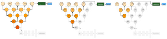
Figure 5.
Illustration of the auto pruning mechanism.
2.3.4. Loss Function
To better adapt to the data set in this paper, we optimize the loss function of the network and use the Exponential Logarithmic Loss proposed in [37]. The specific form is as follows:
The loss function in the above equation consists of two components, represents the Dice loss; represents the CrossEntropy loss. Two parameter weights are added as and respectively, while is the exponential log Dice loss. is the exponential cross-entropy loss. The formula is as follows:
where x denotes the pixel position, i represents the category label, l denotes ground truth category at location l, and represents the probability value after the softmax operation. In addition, , where stands for the frequency of label k’s occurrence. This parameter is used to reduce the weights of categories with a high occurrence rate. and can enhance the nonlinearity of the loss function.
3. Experiment
3.1. Evaluation Metrics
To verify the performance of the model, the following indexes are used as model evaluation indicators in this paper.
- Pixel Accuracy () is the percentage of precisely classified pixels in an image, i.e., the proportion of correctly classified pixels to total pixels. The formula can be expressed as:n denotes the overall number of categories, denotes the category number including backgrounds; expounds the entire number of real pixels whose label is i and is predicted to be class i, i.e., the total number of matched pixels for real pixels whose class is i; indicates the total number of real pixels whose label is i that are predicted to be class j, which can also be interpreted as the number of pixels whose label is i that are misclassified into class j.represents the number of true positives, which is positive in both label and predicted value. represents the number of true negatives, which is negative in both label and predicted value. represents the number of false positives, which is negative in label and positive in predicted value. represents the number of false negatives, which is positive in label and negative in predicted value. Then, is the total number of pixels, and is the number of pixels correctly classified.The Mean Pixel Accuracy (MPA) is a simple enhancement of . Calculate the proportion of pixels accurately identified in each class, and then average the average results.
- Intersection-Over-Union (), also known as the Jaccard index, is defined as the intersection of the predicted segmentation and label divided by the intersection of predicted segmentation and label. This indicator has a value between 0 and 1, with 0 indicating no overlap and 1 indicating complete overlap. The calculation formula for binary classification is:where A represents the ground truth, and B denotes the predicted segmentation.The Mean Intersection over Union () is a typical semantic segmentation measure. It computes the intersection and union ratio of two sets. In the semantic segmentation issue, these two sets of ground truth and predicted segmentation calculate the IoU on each class and then average it.
- Precision (P) is the percentage of samples classified as positive samples in the accurately categorized samples.
- Recall (R) describes the percentage of correctly classified positive samples among all positive samples.
3.2. Experiment Setting
The complete model training and validation process was implemented by a personal computer (processor: Intel(R) i9-10900KF @ 3.7 GHz; operating system: Ubuntu 18.04, 64 bits; memory: 16 GB). The training speed was optimized in Graphics Processing Unit (GPU) mode (NVIDIA RTX 3080 10 GB). We select the Adam optimizer with the initial learning rate such that = . The increment of the learning rate is updated according to the method described in Section 3.3.
3.3. Learning Rate
Warm-up [38] is a training scheme. In the pre-training stage, we first use a low learning rate to train certain epochs or steps, such as four epochs or 10,000 steps. Then, we modify it to a preset learning rate for training. When training begins, the model weights are initialized randomly, and the model’s “level of understanding” of the data is 0. If a larger learning rate is used at the beginning, the model might oscillate.
Warm-up first uses a lower learning rate for training to provide the model with prior knowledge of the data. Then, we use the preset learning rate for training to improve the model’s convergence speed and effect. Eventually, using a small learning rate to proceed with exploration, we shun the loss of local best points. For instance, in the training procedure, we set 0.01 learning rate to train the model until the error is less than 80%, and then set a 0.1 learning rate for training.
The mentioned warm-up is the Constant warm-up. Its disadvantage lies in transforming from a tiny learning rate to a comparatively high learning rate, which may cause the training error to increase suddenly. Consequently, in 2018, Facebook proposed a gradual warm-up to solve this problem. It starts from the initial small learning rate; each step increases slightly until the relatively large learning rate initially set is reached, and then it is adopted to conduct training.
In this paper, warm-up is tested, linearly increasing the learning rate from a tiny value to the preset learning rate and then decaying according to the function law. Meanwhile, warm-up is also tested, linearly increasing the learning rate from a minimal value. After reaching the preset value, it decays according to the function law. For the two pre-training methods, their changes are shown in Figure 6.
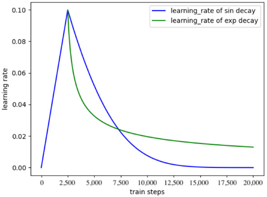
Figure 6.
The warmup learning rate schedule.
4. Results
4.1. Validation Results
Table 1 illustrates the statistical results. The best results of the index are bold. In Table 1, FCN8s [39] has the shortest average running time. The PA, MIoU, P, and R of AttU-Net [40] are 0.9559, 0.9618, 0.9592, and 0.9438, respectively. These indices of AttU-Net are superior to those of FCN series [39], SegNet [41] and VAEU-Net. AttU-Net suggests the spatial attention mechanism to U-Net. VAEU-Net integrates VAE and U-Net to develop the U-Net segmentation effect. Even if VAEU-Net imported VAE, it simply adopts VAE as a portion of the decoder in the last layer. VAEU-Net is barely higher in some indexes than FCN series and SegNet. Our algorithm’s PA, MIoU, P, and R are 0.9737, 0.9745, 0.9646, and 0.9527, respectively.

Table 1.
Comparison with other state-of-the-art algorithms on the segmentation task of medical images.
All of our algorithm’s indices outperform those of the comparison algorithms. Our algorithm is the fourth in terms of average running time. This is caused by the complexity of the generative mask sub-network. Our algorithm delivers the best segmentation impact on the BraTS dataset, according to the results.
4.2. Segmentation Results
For further comparison, we extracted six tomographic images from the 3D sequence of BraTS. These images locate at a considerable distance from each other, fully reflecting the characteristics of this dataset and the difficulty of segmentation. Figure 7, Figure 8, Figure 9, Figure 10, Figure 11, Figure 12, Figure 13, Figure 14 and Figure 15 show the segmentation results. FCN8s, FCN16s, and SegNet lose a multitude of details in the decoding process. The loss of detail delivers these algorithms’ segmentation lines coarse and incorrect at the image edges and details.
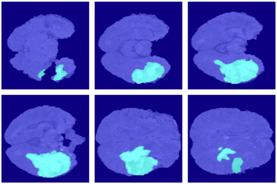
Figure 7.
The ground truth in the BraSt dataset.

Figure 8.
The segmentation results of FCN8s in the BraSt dataset.
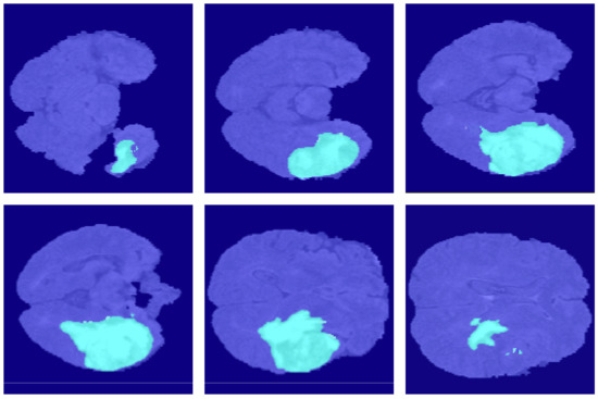
Figure 9.
The segmentation results of FCN16s in the BraSt dataset.

Figure 10.
The segmentation results of FCN32s in the BraSt dataset.
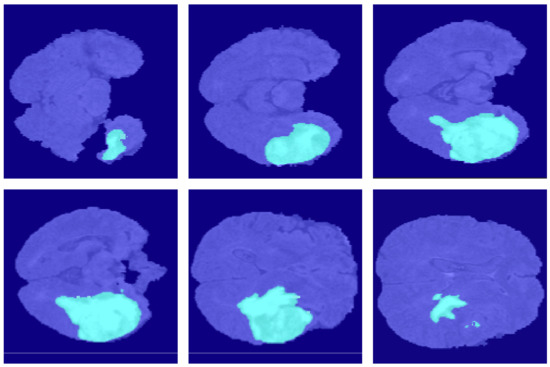
Figure 11.
The segmentation results of U-Net++ in the BraSt dataset.
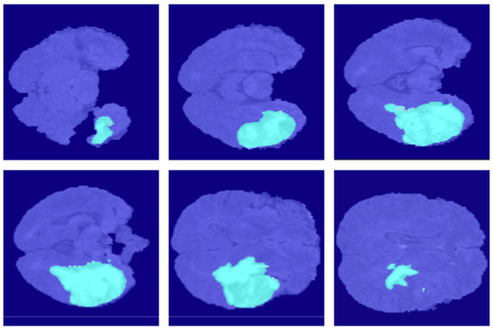
Figure 12.
The segmentation results of SegNet in the BraSt dataset.
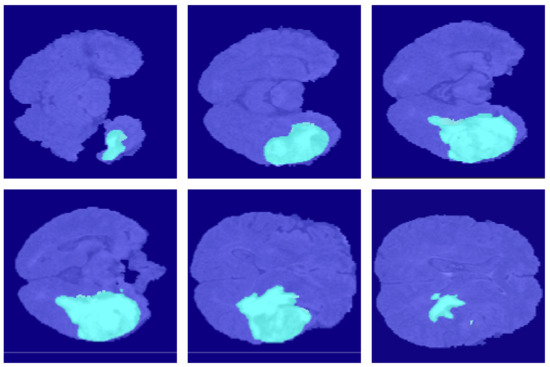
Figure 13.
The segmentation results of AttU-Net in the BraSt dataset.
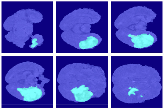
Figure 14.
The segmentation results of VAEU-Net in the BraSt dataset.
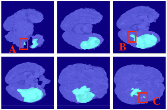
Figure 15.
The segmentation results of GenU-Net++ in the BraSt dataset. Red box A: did not identity the segmentation result. Red box B: the finest segmentation result. Red box C: surpassed comparison models.
As the jump connection compensates for detailed information in decoding, the U-Net segmentation accuracy is increased to some extent. When compared to U-Net++, the segmentation results of AttU-Net, FCN32s, and VAEU-Net improve the segmentation results of most regions, with the exception of the difficult-to-separate regions. Our algorithm is quite good at extracting features. It can also overcome opacity-induced indistinguishability between the target and the background.
That is because our model adds a generative mask sub-network to the last layer of the leading network. This sub-network makes it feasible to learn the features at the edges better by using the properties of generative networks, giving the model a more robust segmentation capability. Therefore, our algorithm yields the most accurate segmentation results. The algorithm in this study produced the most comprehensive segmentation results of any segmentation algorithms.
From Figure 7, Figure 8, Figure 9, Figure 10, Figure 11, Figure 12, Figure 13, Figure 14 and Figure 15, our algorithm’s segmentation results in diverse cases outperformed those of the comparison algorithms. In particular, the three red boxes in Figure 15 show that our algorithm performed exceptionally well in terms of edges and details compared to other models. All the comparison algorithms did not identify the segmentation result in red box A. The segmentation result in red box B is the finest compared with all the comparison algorithms, and the FCN8s and FCN16s had almost no lesions detected in this area. Even though our algorithm’s segmentation result in red box C is not as good as the ground truth algorithm, it surpassed other comparison models. The segmentation results show that our algorithm is accessible, efficient, and excellent.
5. Discussion
5.1. Ablation Experiment of Generative Mask Sub-Network
This paper used three generative models to achieve generative mask sub-network: DCGAN, CVAE, and DCGAN-VAE. To verify their respective implementation effects, ablation experiments are carried out in this paper. Table 2 illustrates the experimental results.
Table 2.
The results of different implements of sub-networks.
From the Table 2, it can be seen that DCGAN-VAE combines the advantages of DCGAN and CVAE, respectively. However, this model inference speed is also the slowest. By comparing the baseline model, we can find that various implementations of the generative mask sub-network effectively promote the GenU-Net++ model’s performance. The PA, MIoU, P, and R of the best performing DCGAN-VAE implementation are 0.9741, 0.9745, 0.9642, and 0.9528, respectively.
5.2. Ablation Experiment of Data Enhancement Methods
In addition to the common data enhancement methods in computer vision tasks, such as random flip, crop, translation, advanced data enhancement methods of random erasure and image mixing are also used in this paper. In order to verify the improvement effect of these methods on model performance, we conducted ablation experiments.
Since the four data enhancement methods, Cutout, CutMix, MixUp, and Mosaic, have more intensive computational complexity than the affine transformation-based methods, they have a more significant impact on the training and inference speed of the model. To verify whether it is worthwhile to use these methods, we compared the effects of different combinations. In addition, we explored whether it is feasible only to use affine transformation-based enhancement methods. The experimental results are shown in Table 3.
Table 3.
The results of different data enhancement methods.
In Table 3, we can witness that each data enhancement method can effectively improve the model’s performance. However, the effects of the CutMix and Mosaic methods are similar, and the effects of using only one of them on the model are almost the same. At the same time, when only using the affine transformation-based data augmentation method, although the speed of the model can be increased to 27.9 ms, the PA, MIoU, Precision, and Recall of the model are only 0.9328, 0.9336, 0.9211, and 0.9207, which is a significant decrease. Thus, considering the model’s training and inference speed characteristics, we used Cutout, CutMix, and MixUp together to guarantee that the model has the best all-around performance.
5.3. Ablation Experiment of Pruning Mechanism
In the inference stage, the auto pruning mechanism proposed in this paper can set the sub-network input to 0 to deactivate the generative mask sub-network and improve the inference speed. The same method is used to prune the U-Net++ network layer by layer. This paper carries out experiments to confirm the variation trend of inference speed and performance when the auto pruning mechanism is applied. The experimental results are displayed in Table 4.
Table 4.
The results of different pruning strategies.
Table 4 reflects that only cutting the sub-network enhances the inference speed slightly in the inference stage. In contrast, it has a significant impact on inference performance. This also proves that the proposed generative mask sub-network is capable of effectively improving the U-Net++ model’s performance.
However, through experiments, it can also be discovered that when layer by layer pruning U-Net++ is carried out, the inference speed can be improved to a certain extent. At the same time, the model performance does not significantly decrease. Consequently, if high performance is pursued, a non-pruning strategy can be used. If high timeliness is pursued, the L3 pruning strategy can be carried out on the model. Moreover, the auto pruning strategy can increase the model inference speed with almost no performance loss.
5.4. Diagnosis System on MacOS
To apply the proposed GenU-Net++ model in practice, we encapsulate the model and build a user-friendly diagnosis system. This system is developed in Swift language, the main functional modules of the software are:
- Patient information search and browsing section. Users can search patient information and review historical patient information through the revision block. In order to facilitate users to use patient data, a remote server is used to connect, and the basic information related to patients and medical image data are stored in the remote server MySQL database. To further improve portability, an interface to connect to the database is set aside so that users can connect to the database when the product is applied.
- Basic medical image viewing function. To further determine the lesion, the user can move and magnify the image.
- A block used to write relevant analysis reports.
All these functional features are shown in Figure 16.
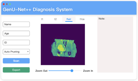
Figure 16.
Diagnosis system interface built on MacOS.
5.5. GenU-Net++ Analysis
The main innovations of the proposed network model can be summarized as the following three points:
- Network structure based on MR image features. MR images have three-dimensional features, and traditional networks extract features from two-dimensional images to achieve tumor segmentation. Due to the extreme similarity of two adjacent two-dimensional images, a 2D network is often not good enough for data feature extraction. Therefore, the basic model of 3D U-Net++ is adopted in this project to extract 3D features from 3D MR images. U-Net structures of different scales are fused into a neural network to strengthen the extraction of 3D features.
- Add generative mask sub-network aiming at solving overfitting in complex network structures. Due to the complexity of neural networks after improvement, the overfitting ability of neural networks will be improved. The model adds a generative mask sub-network branch to find a result of antagonistic generation through the generation model, reducing the possibility of overfitting. The branch calculates the conditional probability distribution of features through the extraction and simulation of features in the highest dimension. The effect of segmenting the same type of tumors is better than that of the decision model. The result is combined with that generated by the upper part of the decision model to calculate the loss, realizing the sub-network regularization and reducing the error of the whole model.
- Two different training modes are under the same model. Generally, the segmentation’s higher accuracy, the better the effect is. However, accuracy improvement often accompanies a considerable time consumption. Moreover, the deepening of neural network depth does not necessarily bring better results. Due to the overfitting, the segmentation result of the deep network may be worse than that of the lower network. Therefore, we propose a second set of solutions for the model. The pruning strategy of U-net++ is used to determine whether pruning should be carried out according to the given conditions during training. The input of the sub-network is set to zero to achieve structural inactivation, which could significantly improve the training speed and even reduce the overfitting of the neural network, leading to the “dual-use of one model”.
5.6. Limitation
Even though our algorithm delivers the best segmentation effect, it has a few drawbacks. As shown in Figure 15, even if our algorithm has been able to segment most of the lesions, it is not sufficiently accurate for such relatively independent and small lesions in boxes A and C. The flaw is a task that we will further have to struggle with in the future.
5.6.1. Segmentation Boundary Loss
The algorithm proposed in this paper still does not work satisfactorily at the boundaries of brain tumors Figure 17. Although the mask information generated by the generative network can enhance the algorithm’s robustness to a certain extent, the results thus far are still not excellent enough. On the one hand, that is due to the failure to assign a higher weight to pixels at boundaries when constructing the loss function. On the other hand, it is difficult for even human beings to quickly determine the boundary lines of some complex images during processing.
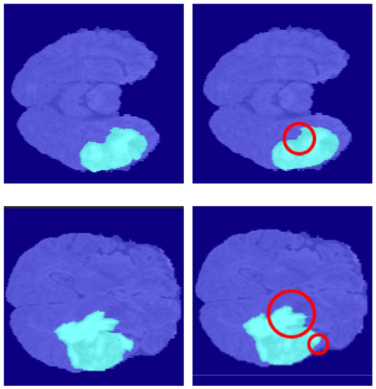
Figure 17.
The limitation of our methods. The left is ground truth, and the right is the predicted segmentation by our methods.
5.6.2. Third Dimensional Information Loss
In this paper, we used a 3D image series, which contained the three-dimensional information of the whole lesion. However, this information was not fully utilized in this paper, as it was still treated as multiple consecutive two-dimensional images. Hence, the continuity and correlation information in the third dimension is not fully utilized in this way. When the processed lesion images appear for the first time in one image and gradually expand in the subsequent images, theoretically, the segmentation effect of these images will be effectively improved if the continuity information in the third dimension contained in the 3D images series is fully utilized.
5.7. Future Work
As described in Section 5.6, the method proposed in this paper still does not work well at the boundaries of the brain tumor segmentation. The dataset used in this paper is a slice sequence, which is three-dimensional image information. Nevertheless, the current algorithm does not effectively utilize the continuity in the three-dimension to optimize the segmentation results. Therefore, the authors of this paper optimize the proposed generative mask sub-network to extract the continuity and correlation features in three-dimensional space to optimize the segmentation results further.
6. Conclusions
The brain tumor is a lethal neoplasm that grows in the brain and horribly impacts the essential functionalities of the brain. Brain tumor segmentation has occupied a critical status in the computational biomedical fields in recent years. This paper uses the BraTS 2018 dataset, comprising 245 patients’ MR images. Moreover, MRI segmentation currently has difficulties as follows. 1. The requirement of a discernible difference in the brightness of the detection target compared to the background. 2. The MRI has blurred boundaries, semblable gray values, and low contrast. 3. Eliminating noise has an influence on the image information details. Therefore, this paper proposes a segmentation algorithm based on U-Net++, aiming to address these mentioned above problems.
This paper introduced the generative mask sub-network and auto pruning mechanism—specifically: 1. A generative mask sub-network generated feature maps using BiCubic interpolation to conduct upsampling and obtains segmentation results different from U-Net++. Then, this paper employed pixel-weighted fusion to fuse the two segmentation results. Through this process, the robustness and segmentation performance of the model were improved.
2. We proposed an auto pruning mechanism that depended on the architectural characteristics of U-Net++. This mechanism deactivated the sub-network by zeroing the input. It also automatically pruned GenU-Net++ during the inference process, increasing the inference speed and improving the network performance by preventing overfitting. Ultimately, on the validation set, the proposed method reached 0.9737, 0.9745, 0.9646, and 0.9527 on the PA, MIoU, P, and R indices, respectively. This experimental result demonstrates that the proposed model surpassed all the compared models.
In order to verify the effectiveness of various implementations of generative mask sub-networks, in Section 5, we tested the performance of DCGAN, CVAE, and DCGAN-VAE, respectively. The sub-network implemented on DCGAN-VAE had the best performance without considering the inference speed. We also tested different levels of pruning strategies. The results indicate that the proposed auto pruning mechanism was able to balance the model’s performance with the inference speed. Moreover, it could still take advantage of the generative mask sub-network with an inference speed close to the native U-Net++.
Although the proposed model surpassed the comparison model, limitations were still present. First, the algorithm was still not good enough in the boundary region of brain tumors. Second, the model has been adapted for 3D image sequences; however, it still cannot make good use of the 3D information in the dataset. These shortcomings are future directions for the authors of this paper. Ultimately, this paper encapsulated the model and developed a corresponding application under the MacOS platform, thus, making the model applicable.
Author Contributions
Conceptualization, Y.Z.; methodology, Y.Z.; validation, Y.Z.; writing—original draft preparation, Y.Z.; writing—review and editing, Y.Z., S.W., X.L. and Y.L.; visualization, Y.Z. and J.K.; supervision, Y.Z.; project administration, C.L.; funding acquisition, C.L. All authors have read and agreed to the published version of the manuscript.
Funding
This research was funded by National Natural Science Foundation of China grant number 61202479.
Institutional Review Board Statement
Not applicable.
Informed Consent Statement
Not applicable.
Data Availability Statement
Not applicable.
Acknowledgments
We are grateful to the Edison Coding Club of CIEE in China Agricultural University for their strong support during our thesis writing.
Conflicts of Interest
The authors declare no conflict of interest.
References
- Gurbină, M.; Lascu, M.; Lascu, D. Tumor Detection and Classification of MRI Brain Image using Different Wavelet Transforms and Support Vector Machines. In Proceedings of the 2019 42nd International Conference on Telecommunications and Signal Processing (TSP), Budapest, Hungary, 1–3 July 2019; pp. 505–508. [Google Scholar] [CrossRef]
- Qin, P.; Zhang, J.; Zeng, J.; Liu, H.; Cui, Y. A framework combining DNN and level-set method to segment brain tumor in multi-modalities MR image. Soft Comput. 2019, 23, 9237–9251. [Google Scholar] [CrossRef]
- Pedro, M.T.; Eissler, A.; Schmidberger, J.; Kratzer, W.; Wirtz, C.R.; Antoniadis, G.; Koenig, R.W. Sodium Fluorescein–Guided Surgery in Peripheral Nerve Sheath Tumors: First Experience in 10 Cases of Schwannoma. World Neurosurg. 2019, 124, e724–e732. [Google Scholar] [CrossRef]
- Fyllingen, E.H.; Bø, L.E.; Reinertsen, I.; Jakola, A.S.; Sagberg, L.M.; Berntsen, E.M.; Salvesen, Ø.; Solheim, O. Survival of glioblastoma in relation to tumor location: A statistical tumor atlas of a population-based cohort. Acta Neurochir. 2021, 163, 1895–1905. [Google Scholar] [CrossRef]
- Shivaprasad, B.J.; Ravikumar, M.; Guru, D.S. Analysis of Brain Tumor Using MR Images: A Brief Survey. Int. J. Image Graph. 2021. [Google Scholar] [CrossRef]
- Zhang, C.; Shen, X.; Cheng, H.; Qian, Q. Brain tumor segmentation based on hybrid clustering and morphological operations. Int. J. Biomed. Imaging 2019, 2019, 7305832. [Google Scholar] [CrossRef]
- Zhang, D.; Huang, G.; Zhang, Q.; Han, J.; Yu, Y. Cross-Modality Deep Feature Learning for Brain Tumor Segmentation. Pattern Recognit. 2020, 110, 107562. [Google Scholar] [CrossRef]
- Hossain, T.; Shishir, F.S.; Ashraf, M.; Al Nasim, M.A.; Shah, F.M. Brain tumor detection using convolutional neural network. In Proceedings of the 2019 1st International Conference on Advances in Science, Engineering and Robotics Technology (ICASERT), Dhaka, Bangladesh, 3–5 May 2019; pp. 1–6. [Google Scholar]
- Thaha, M.M.; Kumar, K.P.M.; Murugan, B.; Dhanasekeran, S.; Vijayakarthick, P.; Selvi, A.S. Brain tumor segmentation using convolutional neural networks in MRI images. J. Med. Syst. 2019, 43, 294. [Google Scholar] [CrossRef]
- Tiwari, A.; Srivastava, S.; Pant, M. Brain tumor segmentation and classification from magnetic resonance images: Review of selected methods from 2014 to 2019. Pattern Recognit. Lett. 2020, 131, 244–260. [Google Scholar] [CrossRef]
- Roy, M.; Mali, K.; Chatterjee, S.; Chakraborty, S.; Debnath, R.; Sen, S. A study on the applications of the biomedical image encryption methods for secured computer aided diagnostics. In Proceedings of the 2019 Amity International Conference on Artificial Intelligence (AICAI), Dubai, United Arab Emirates, 4–6 February 2019; pp. 881–886. [Google Scholar]
- Du, G.; Cao, X.; Liang, J.; Chen, X.; Zhan, Y. Medical image segmentation based on u-net: A review. J. Imaging Sci. Technol. 2020, 64, 20508-1–20508-12. [Google Scholar] [CrossRef]
- Falk, T.; Mai, D.; Bensch, R.; Çiçek, Ö.; Abdulkadir, A.; Marrakchi, Y.; Böhm, A.; Deubner, J.; Jäckel, Z.; Seiwald, K.; et al. U-Net: Deep learning for cell counting, detection, and morphometry. Nat. Methods 2019, 16, 67–70. [Google Scholar] [CrossRef]
- Khanna, A.; Londhe, N.D.; Gupta, S.; Semwal, A. A deep Residual U-Net convolutional neural network for automated lung segmentation in computed tomography images. Biocybern. Biomed. Eng. 2020, 40, 1314–1327. [Google Scholar] [CrossRef]
- Ghosh, S.; Chaki, A.; Santosh, K. Improved U-Net architecture with VGG-16 for brain tumor segmentation. Phys. Eng. Sci. Med. 2021, 44, 703–712. [Google Scholar] [CrossRef]
- Xz, A.; Xl, B.; Kai, H.A.; Yuan, Z.A.; Zc, C.; Xga, D. ERV-Net: An efficient 3D residual neural network for brain tumor segmentation—ScienceDirect. Expert Syst. Appl. 2021, 170, 114566. [Google Scholar]
- Sun, L.; Zhang, S.; Chen, H.; Luo, L. Brain tumor segmentation and survival prediction using multimodal MRI scans with deep learning. Front. Neurosci. 2019, 13, 810. [Google Scholar] [CrossRef] [Green Version]
- Naveena, C.; Poornachandra, S.; Aradhya, V.M. Segmentation of Brain Tumor Tissues in Multi-channel MRI Using Convolutional Neural Networks. In International Conference on Brain Informatics; Springer: Cham, Switzerland, 2020; pp. 128–137. [Google Scholar]
- Chen, S.; Ding, C.; Liu, M. Dual-force convolutional neural networks for accurate brain tumor segmentation. Pattern Recognit. 2019, 88, 90–100. [Google Scholar] [CrossRef]
- Alqazzaz, S.; Sun, X.; Yang, X.; Nokes, L. Automated brain tumor segmentation on multi-modal MR image using SegNet. Comput. Vis. Media 2019, 5, 209–219. [Google Scholar] [CrossRef] [Green Version]
- Ramya, P.; Thanabal, M.S.; Dharmaraja, C. Brain tumor segmentation using cluster ensemble and deep super learner for classification of MRI. J. Ambient. Intell. Humaniz. Comput. 2021, 12, 9939–9952. [Google Scholar] [CrossRef]
- Huang, Z.; Liu, Y.; Song, G.; Zhao, Y. GammaNet: An Intensity-Invariance Deep Neural Network for Computer-aided Brain Tumor Segmentation. Opt.-Int. J. Light Electron Opt. 2021, 243, 167441. [Google Scholar] [CrossRef]
- MICCAI. BraTS 2018. Available online: http://braintumorsegmentation.org (accessed on 1 December 2021).
- Krizhevsky, A.; Sutskever, I.; Hinton, G. ImageNet Classification with Deep Convolutional Neural Networks. Adv. Neural Inf. Process. Syst. 2012, 25, 1097–1105. [Google Scholar] [CrossRef]
- Zhang, H.; Cisse, M.; Dauphin, Y.N.; Lopez-Paz, D. mixup: Beyond empirical risk minimization. arXiv 2017, arXiv:1710.09412. [Google Scholar]
- DeVries, T.; Taylor, G.W. Improved regularization of convolutional neural networks with cutout. arXiv 2017, arXiv:1708.04552. [Google Scholar]
- Yun, S.; Han, D.; Oh, S.J.; Chun, S.; Choe, J.; Yoo, Y. Cutmix: Regularization strategy to train strong classifiers with localizable features. In Proceedings of the IEEE/CVF International Conference on Computer Vision, Seoul, Korea, 27–28 October 2019; pp. 6023–6032. [Google Scholar]
- Zhou, Z.; Siddiquee, M.M.R.; Tajbakhsh, N.; Liang, J. Unet++: A nested u-net architecture for medical image segmentation. In Deep Learning in Medical Image Analysis and Multimodal Learning for Clinical Decision Support; Springer: Berlin/Heidelberg, Germany, 2018; pp. 3–11. [Google Scholar]
- Pateria, A.; Vyas, V.; Pratyush, M. Enhanced Image Capturing Using CNN. 1990. Available online: https://www.researchgate.net/publication (accessed on 1 December 2021).
- Radford, A.; Metz, L.; Chintala, S. Unsupervised representation learning with deep convolutional generative adversarial networks. arXiv 2015, arXiv:1511.06434. [Google Scholar]
- Kingma, D.P.; Welling, M. Auto-encoding variational bayes. arXiv 2013, arXiv:1312.6114. [Google Scholar]
- Bao, J.; Chen, D.; Wen, F.; Li, H.; Hua, G. CVAE-GAN: Fine-grained image generation through asymmetric training. In Proceedings of the IEEE International Conference on Computer Vision, Venice, Italy, 27–29 October 2017; pp. 2745–2754. [Google Scholar]
- Neubeck, A.; Van Gool, L. Efficient non-maximum suppression. In Proceedings of the 18th International Conference on Pattern Recognition (ICPR’06), Hong Kong, China, 20–24 August 2006; Volume 3, pp. 850–855. [Google Scholar]
- Solovyev, R.; Wang, W.; Gabruseva, T. Weighted boxes fusion: Ensembling boxes for object detection models. arXiv 2019, arXiv:1910.13302. [Google Scholar] [CrossRef]
- Ronneberger, O.; Fischer, P.; Brox, T. U-net: Convolutional networks for biomedical image segmentation. In International Conference on Medical Image Computing and Computer-Assisted Intervention; Springer: Berlin/Heidelberg, Germany, 2015; pp. 234–241. [Google Scholar]
- Hu, J.; Shen, L.; Sun, G. Squeeze-and-excitation networks. In Proceedings of the IEEE Conference on Computer Vision and Pattern Recognition, Salt Lake City, UT, USA, 18–23 June 2018; pp. 7132–7141. [Google Scholar]
- Wong, K.C.; Moradi, M.; Tang, H.; Syeda-Mahmood, T. 3D segmentation with exponential logarithmic loss for highly unbalanced object sizes. In International Conference on Medical Image Computing and Computer-Assisted Intervention; Springer: Cham, Switzerland, 2018; pp. 612–619. [Google Scholar]
- He, K.; Zhang, X.; Ren, S.; Sun, J. Deep Residual Learning for Image Recognition. In Proceedings of the 2016 IEEE Conference on Computer Vision and Pattern Recognition (CVPR), Las Vegas, NV, USA, 27–30 June 2016. [Google Scholar]
- Long, J.; Shelhamer, E.; Darrell, T. Fully convolutional networks for semantic segmentation. In Proceedings of the IEEE Conference on Computer Vision and Pattern Recognition, Boston, MA, USA, 7–12 June 2015; pp. 3431–3440. [Google Scholar]
- Oktay, O.; Schlemper, J.; Folgoc, L.L.; Lee, M.; Heinrich, M.; Misawa, K.; Mori, K.; McDonagh, S.; Hammerla, N.Y.; Kainz, B.; et al. Attention u-net: Learning where to look for the pancreas. arXiv 2018, arXiv:1804.03999. [Google Scholar]
- Badrinarayanan, V.; Kendall, A.; Cipolla, R. Segnet: A deep convolutional encoder-decoder architecture for image segmentation. IEEE Trans. Pattern Anal. Mach. Intell. 2017, 39, 2481–2495. [Google Scholar] [CrossRef] [PubMed]
Publisher’s Note: MDPI stays neutral with regard to jurisdictional claims in published maps and institutional affiliations. |
© 2021 by the authors. Licensee MDPI, Basel, Switzerland. This article is an open access article distributed under the terms and conditions of the Creative Commons Attribution (CC BY) license (https://creativecommons.org/licenses/by/4.0/).