Article

GomJau-Hogg’s Notation for Automatic Generation of k-Uniform Tessellations with ANTWERP v3.0

1
Department of Geographic Engineering and Graphical Expression Techniques, Universidad de Cantabria, 39005 Santander, Spain
2
Spotify, London WC2N 6AT, UK
*
Author to whom correspondence should be addressed.
Symmetry 2021, 13(12), 2376; https://doi.org/10.3390/sym13122376
Submission received: 30 October 2021 / Revised: 1 December 2021 / Accepted: 6 December 2021 / Published: 9 December 2021
(This article belongs to the Special Issue Recent Advances in Software for Symmetry)

Abstract

:
Euclidean tilings are constantly applied to many fields of engineering (mechanical, civil, chemical, etc.). These tessellations are usually named after Cundy & Rollett’s notation. However, this notation has two main problems related to ambiguous conformation and uniqueness. This communication explains the GomJau-Hogg’s notation for generating all the regular, semi-regular (uniform) and demi-regular (k-uniform, up to at least k = 3) in a consistent, unique and unequivocal manner. Moreover, it presents Antwerp v3.0, a free online application, which is publicly shared to prove that all the basic tilings can be obtained directly from the GomJau-Hogg’s notation.

1. Introduction

Euclidean tiling is the covering of a plane where the repetition of regular polygons make up tiles, which through symmetry operations can be extended indefinitely without any overlapping [1]. There are three types of tilings:
  • Regular tilings consist of a single polygon type, with each vertex surrounded by the same kinds of polygons (vertex-transitive) (Figure 1). There are only 3 of them, having six equilateral triangles (Figure 1a), four squares (Figure 1b) or three regular hexagons (Figure 1c) at any vertex.
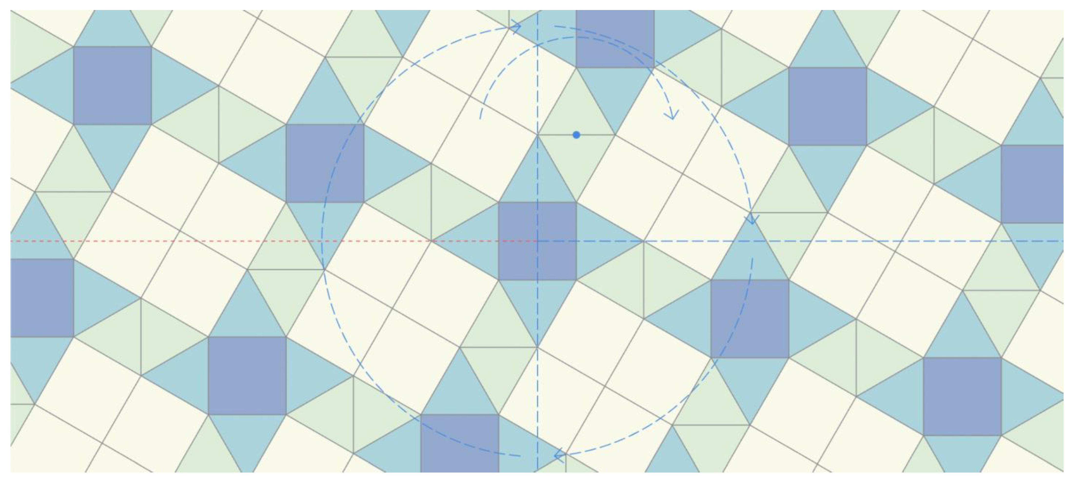
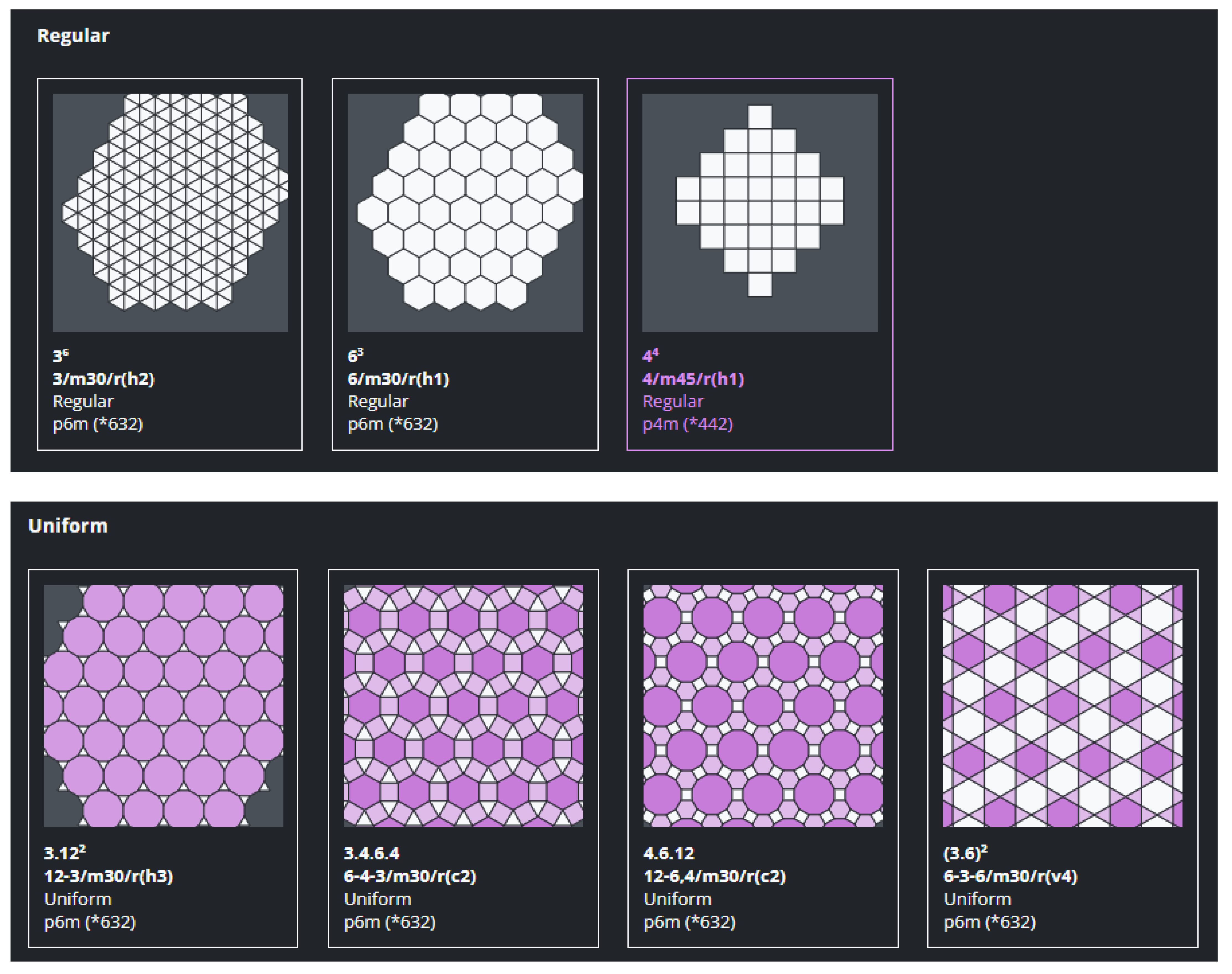
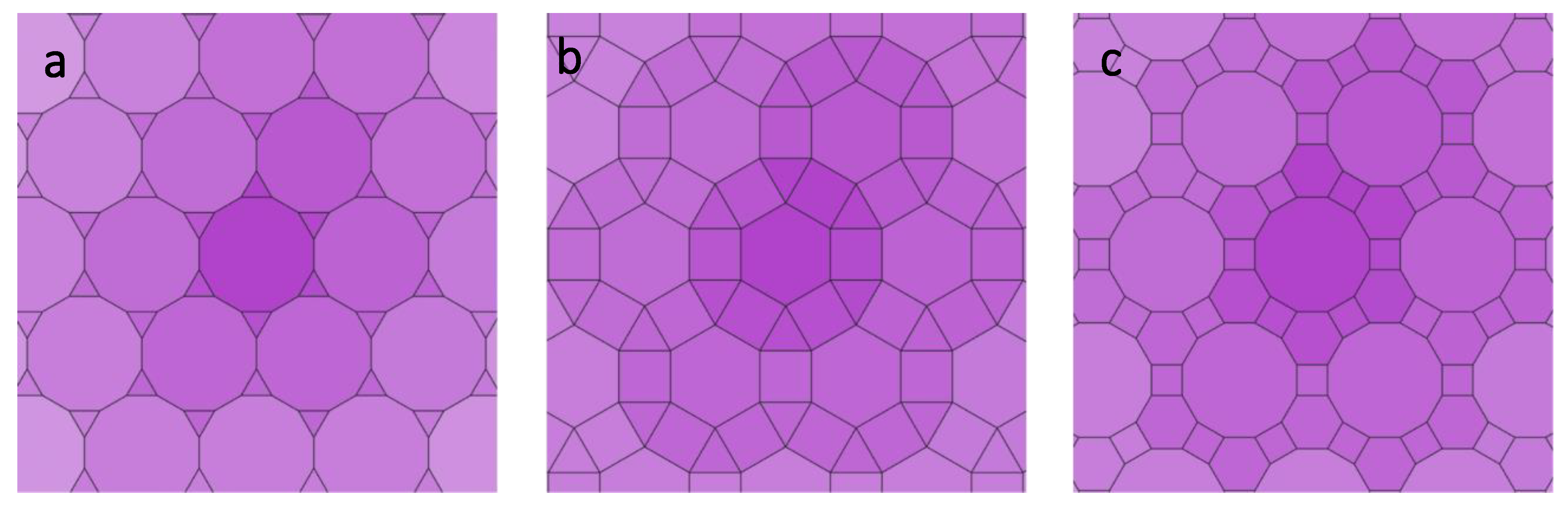
  • Semi-regular tilings (Archimedean or uniform) are polymorphic (several polygon types) and also vertex-transitive (Figure 2). There are only 8 of them.
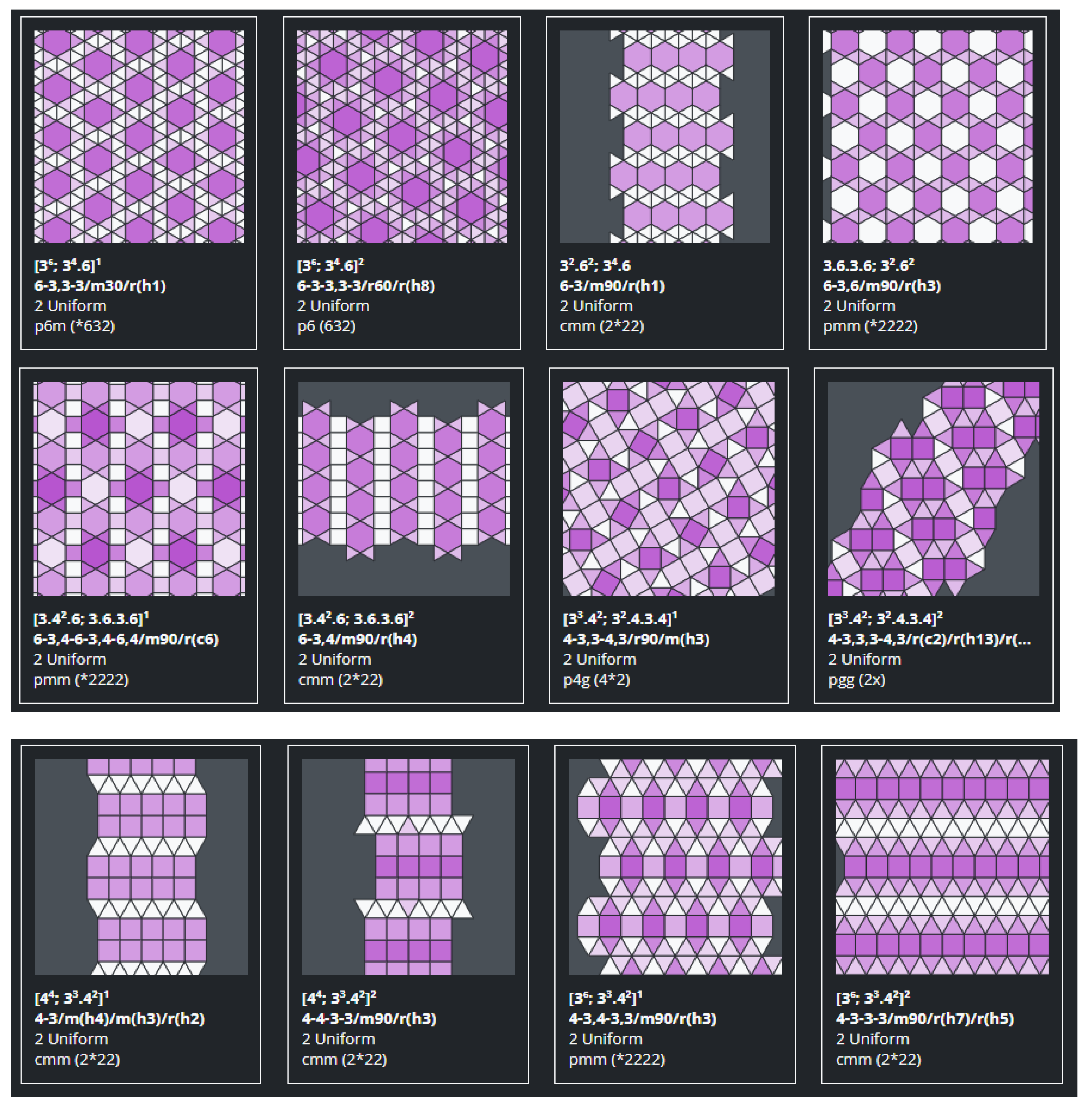
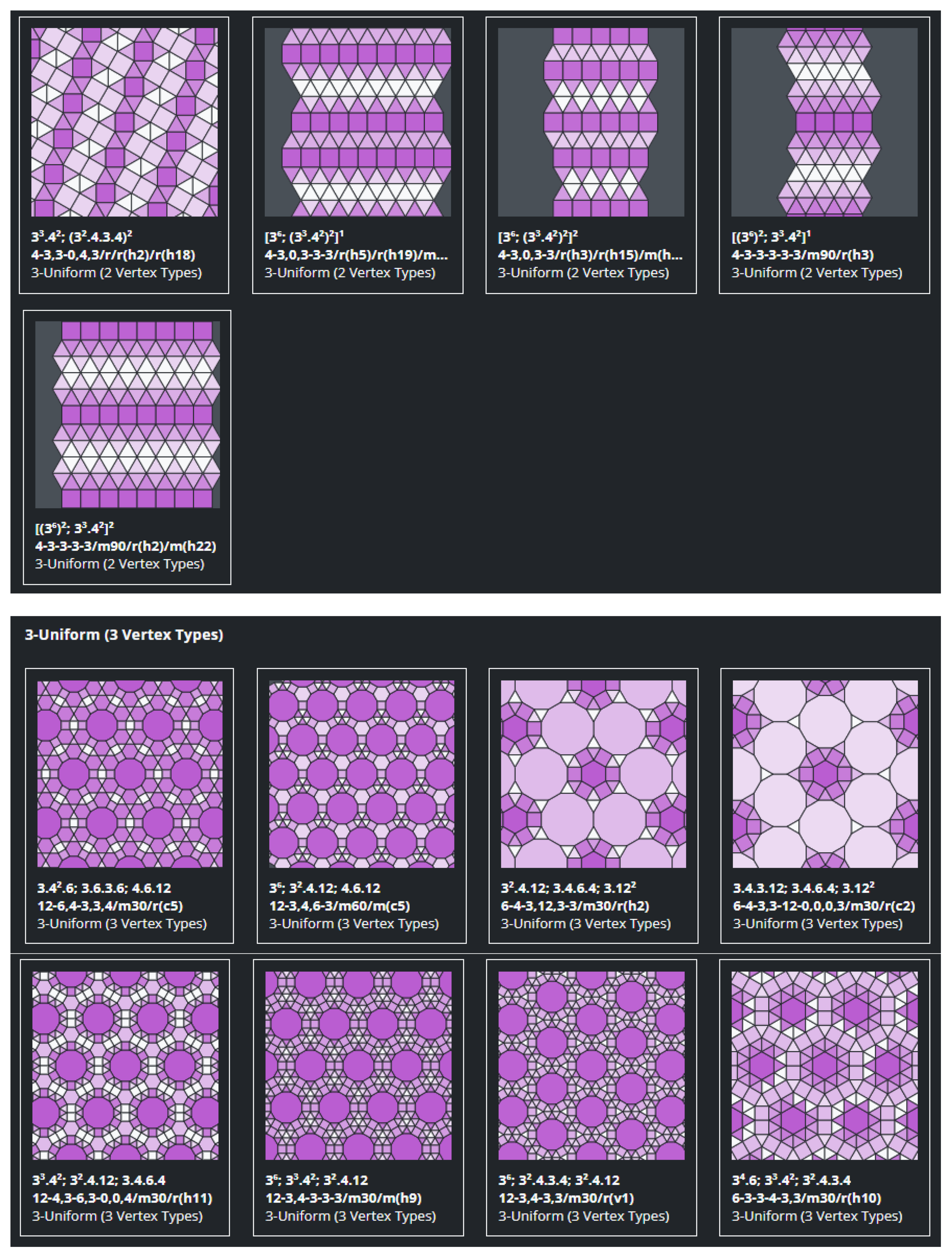
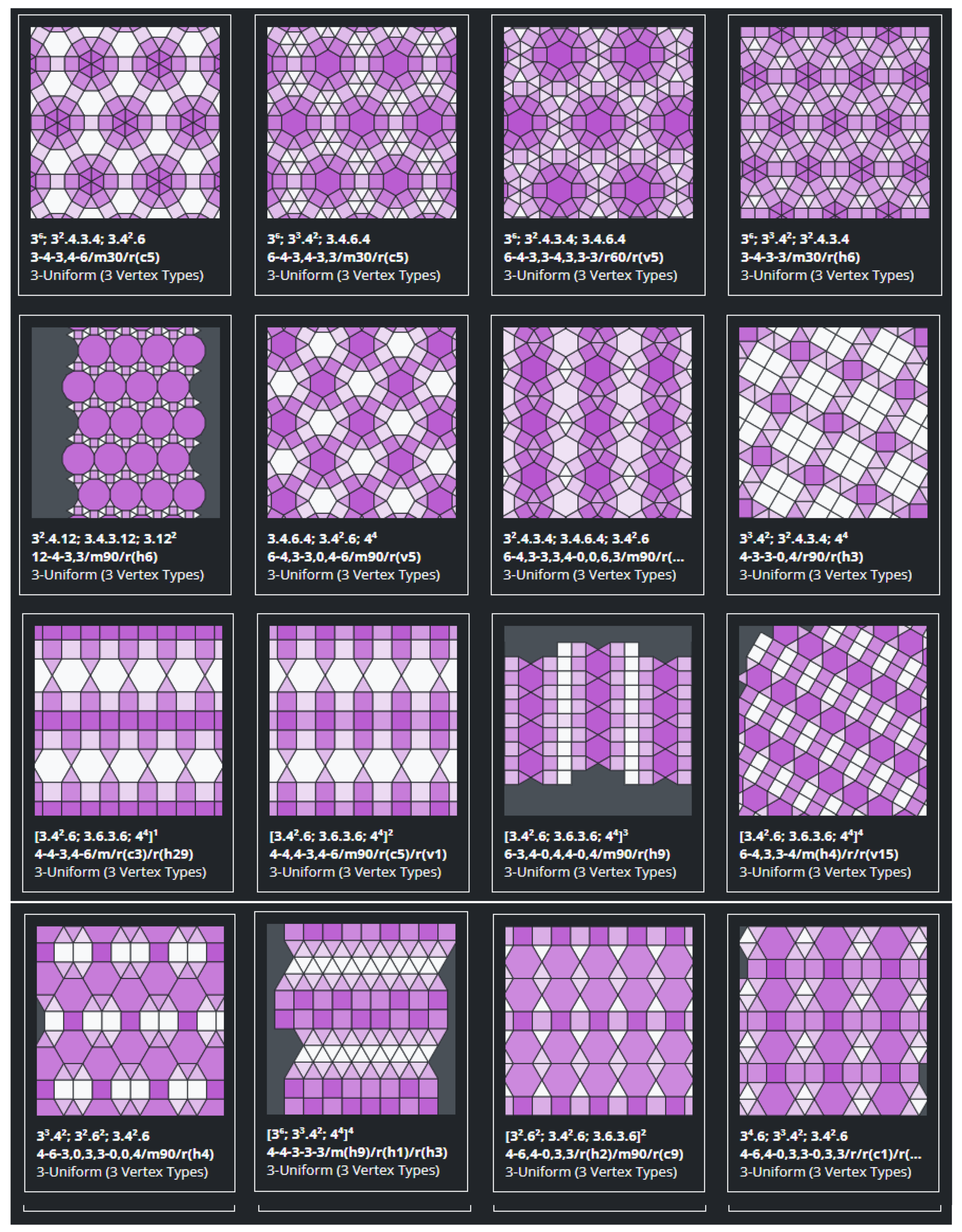
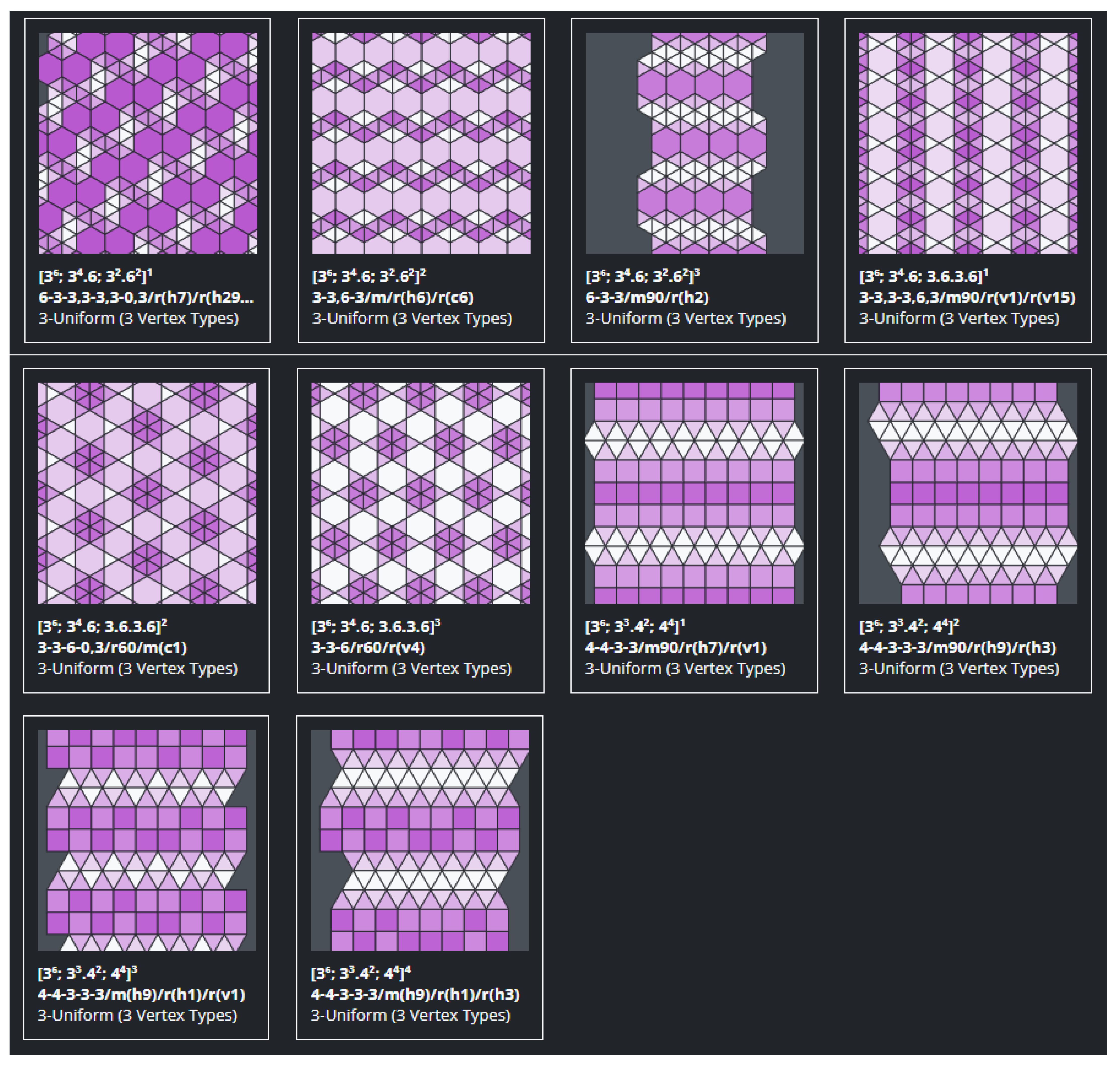
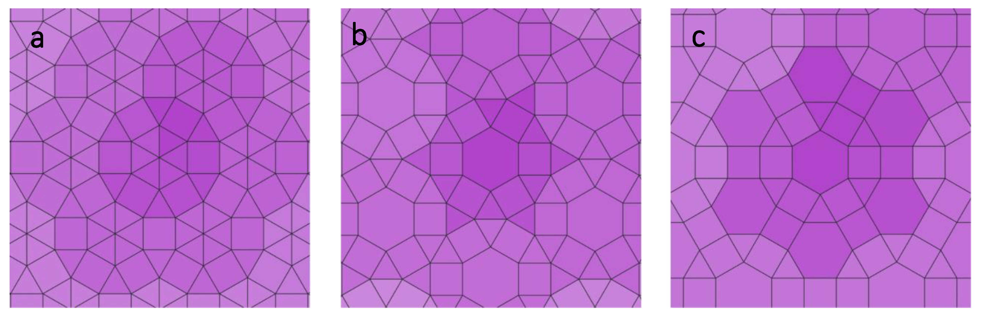
  • Demi-regular tilings (k-uniform) like semi-regular tilings are polymorphic but are not vertex-transitive (Figure 3). For instance, there are 20 2-uniform tessellations and there are 61 3-uniform (22 are 2-vertex and 39 are 3-vertex types).
Tiling configurations are usually named using Cundy & Rollett’s notation [2], which adapted the Schläfli symbol. This notation represents (i) the number of vertices, (ii) the number of polygons around each vertex (arranged clockwise) and (iii) the number of sides to each of those polygons. For example: 36; 36; 34.6, tells us there are 3 vertices with 2 different vertex types, so this tiling would be classed as a ‘3-uniform (2-vertex types)’ tiling. Broken down, 36; 36 (both of different transitivity class), or (36)2, tells us that there are 2 vertices (denoted by the superscript 2), each with 6 equilateral 3-sided polygons (triangles). With a final vertex 34.6, 4 more contiguous equilateral triangles and a single regular hexagon.

2. Problems of Cundy & Rollett Notation

The Cundy & Rollett notation has two main problems. First, when it comes to k-uniform tilings, the notation does not explain the relationships between the vertices. This makes it impossible to generate a covered plane given the notation alone. Let us take the above notation as an example, (36)2; 34.6: If a single vertex was placed, surrounded by 4 triangles and a hexagon (34.6), there would be 3 other vertices with 2 triangles (A, B and C in Figure 4c). From here, either the vertex type of 36 (as shown if Figure 4b) or 34.6 (Figure 4c) is possible, and the notation gives no indication to which is correct.
All three tessellations, with the same nomenclature, are represented in Figure 5. The tilings are very similar but it can be noticed that the relative positions of the hexagons are different. Therefore, the second problem is that this nomenclature is not unique for each tessellation [3].

3. GomJau-Hogg’s Notation: A New Notation

Here we present the GomJau-Hogg’s notation, a slightly modified version of the research and notation presented by Gómez-Jáuregui et al. [3], about the generation and nomenclature of tessellations and double-layer grids. The origin of that notation is inspired by Otero’s work [1] about domes and spatial frames. The present work allows for the infinite generation of regular polygon tilings through a set of shape placement stages and iterative rotation and reflection operations.
Several examples will be used in the following sections. The above mentioned (36)2; 34.6 (the first of the three variants) is translated to 6-3-3/m30/r(v3). The stages are represented as blocks separated by a forward-slash (/). When split up, the very first block is the “Shape placement” stage, which takes care of placing the first regular polygons on the plane. The blocks after this are the transformation functions, of which there will be two or more.

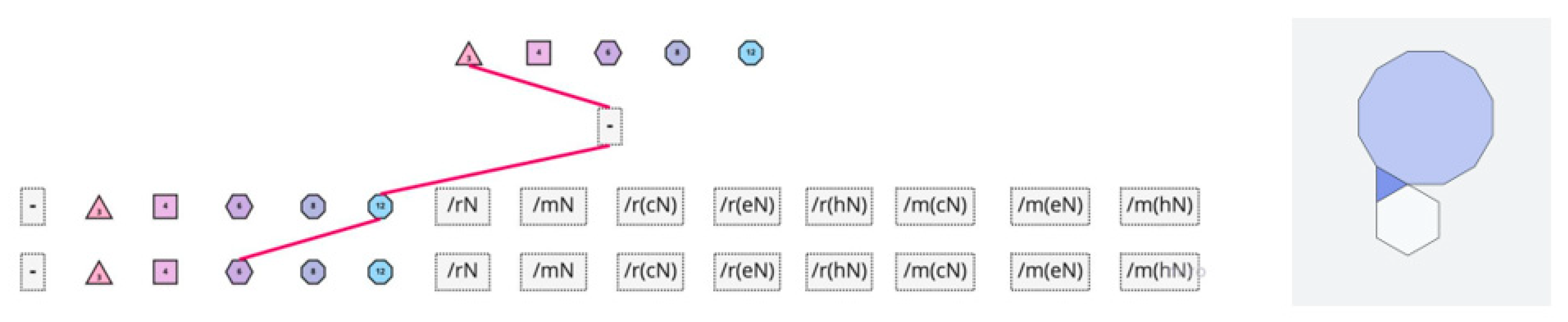
3.1. Stage 1: Polygon Placement

The shape placement stage is made up of a series of hyphen (-) separated phases. Similar to the Cundy & Rollett’s notation, each number represents the number of sides on the polygon.
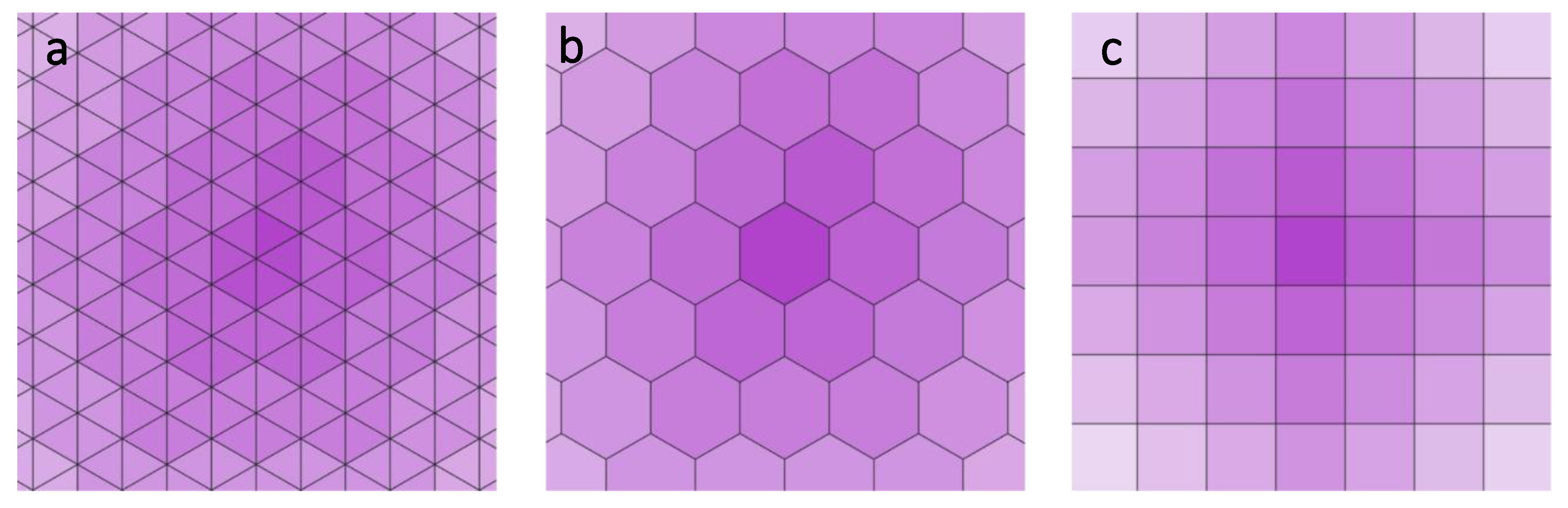
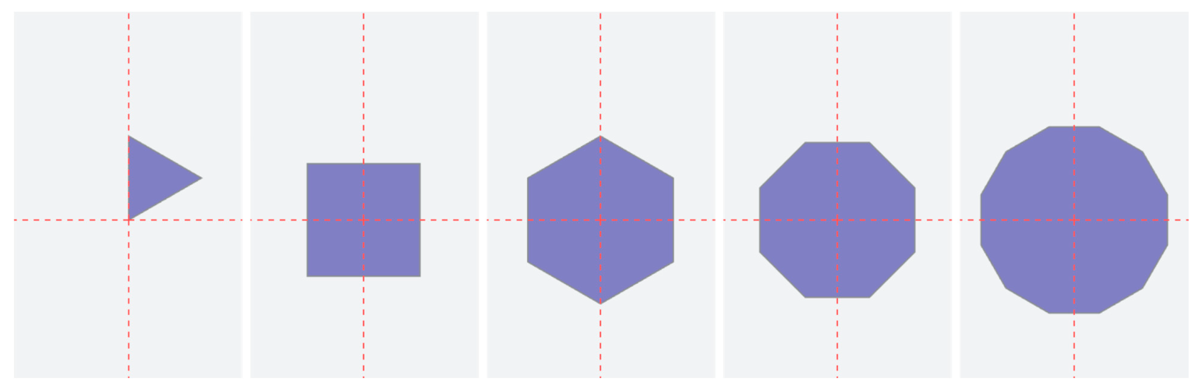
  • Phase 1 (seed polygon phase): The very first phase will always contain a single number of either 3, 4, 6, 8 or 12. This is because there are seventeen combinations of regular polygons whose internal angles add up to 360°, however only eleven of these can occur in regular polygon tilings [4]. This defines the ‘seed polygon’, which is the first shape to be placed at the origin of the area to be covered.
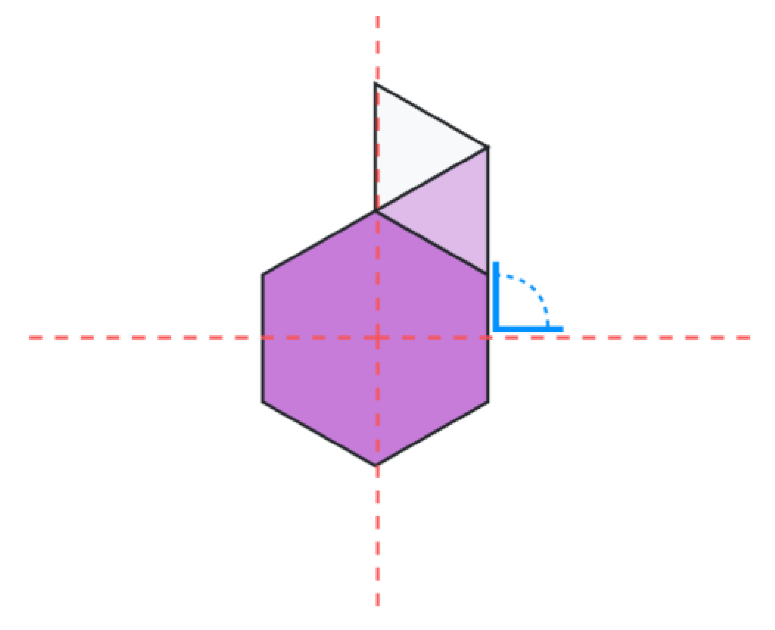
  • The seed polygon is always (except for the 3-sided polygon, equilateral triangle) placed at the origin of the plane so that the two sides that intersect the horizontal axis “x”, stay perpendicular to that axis (Figure 6). For an equilateral triangle the left-hand edge will be the one perpendicular to the x axis and will be aligned with the vertical axis ‘y’ [3] (Figure 7).
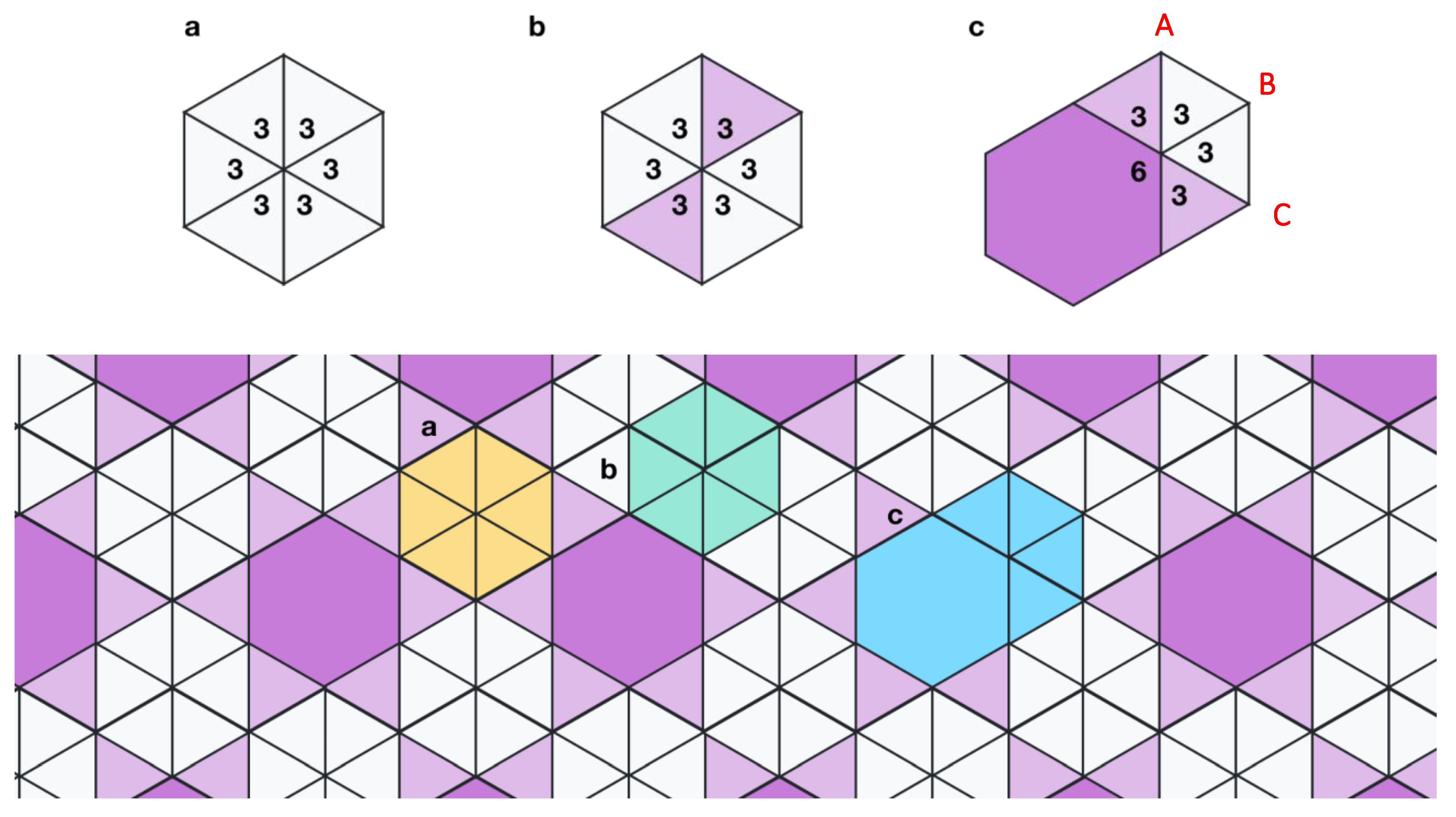
  • Phase 2: Following the first phase, regular polygons are systematically placed clockwise around the available sides of the seed polygon, using 0 to skip a side of a polygon. The principle is to first fill the upper right quadrant and then move clockwise.
  • Phase 3 (and 4, 5, etc.): Regular polygons are systematically placed clockwise around the available sides of the polygons placed in the previous phase, in the same manner as in phase 2.
Let us use the above configuration example, (36)2; 34.6 in its former notation, which would become GomJau-Hogg’s notation 6-3-3/m30/r(v3) (Figure 6). With this new notation as shown above, the polygon placement stage (6-3-3) consists of:
  • A seed polygon with 6 sides. In Figure 6, hexagon in dark blue.
  • A following phase with a three-sided shape; placed on the first side clockwise of the y axis. In Figure 6, equilateral triangle in light blue.
  • Followed by a final phase of one triangle; placed on the first available side clockwise, of the previously placed triangle. In Figure 6, equilateral triangle in white.

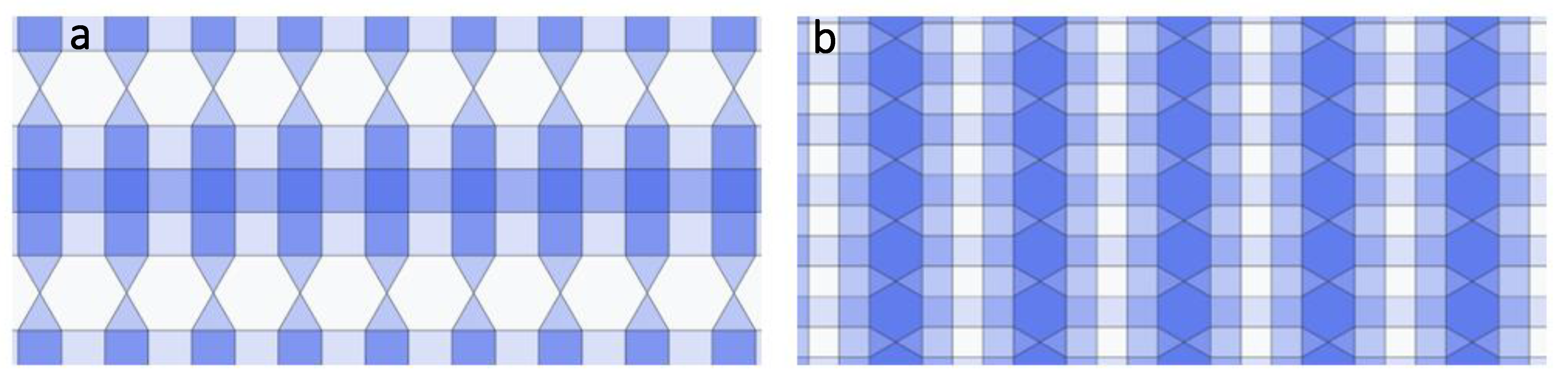
3.2. Stage 2: First Transformation Function

The stages following the first polygon placement stage are a series of transformation functions that take all of the shapes currently placed on the plane. It is necessary to define 3 parameters for each transformation: the type of transformation, the angle and the origin.
  • Type of transformation: It is represented in the notation by a single character. An ‘m’ (mirror) applies a reflection transformation and a ‘r’ applies a rotation transformation.
  • Angle: When we have the polygons of the first stage, it is necessary to either rotate or reflect them by a specified angle. When no angle is specified it defaults to 180°.
  • Origin: The origin of the transformation is specified between parentheses. When no origin is specified it defaults to the center of the coordinate system. There are 2 types of transformation origins, explained in the following lines.

3.2.1. Origin 1. Center of the Coordinate System—Continuous Centered Transformation

This is the default origin type (it is not defined between parentheses) and, when used, the transformation is applied continuously by incrementing the angle on each transformation by a factor of 2. This is done while the accumulated angle is less than a full rotation on the plane (e.g., 360°). This is the case for both mirroring (m) and rotation (r) transforms. With every iteration of the transform, all shapes on the plane including those from previous iterations of the same transform are then duplicated (there may be overlapping of a polygon over the same shape, which would be automatically merged). Let us again take the previous example, 6-3-3/m30/r(v3) in order to explain the meaning of m30, shown in Figure 8:
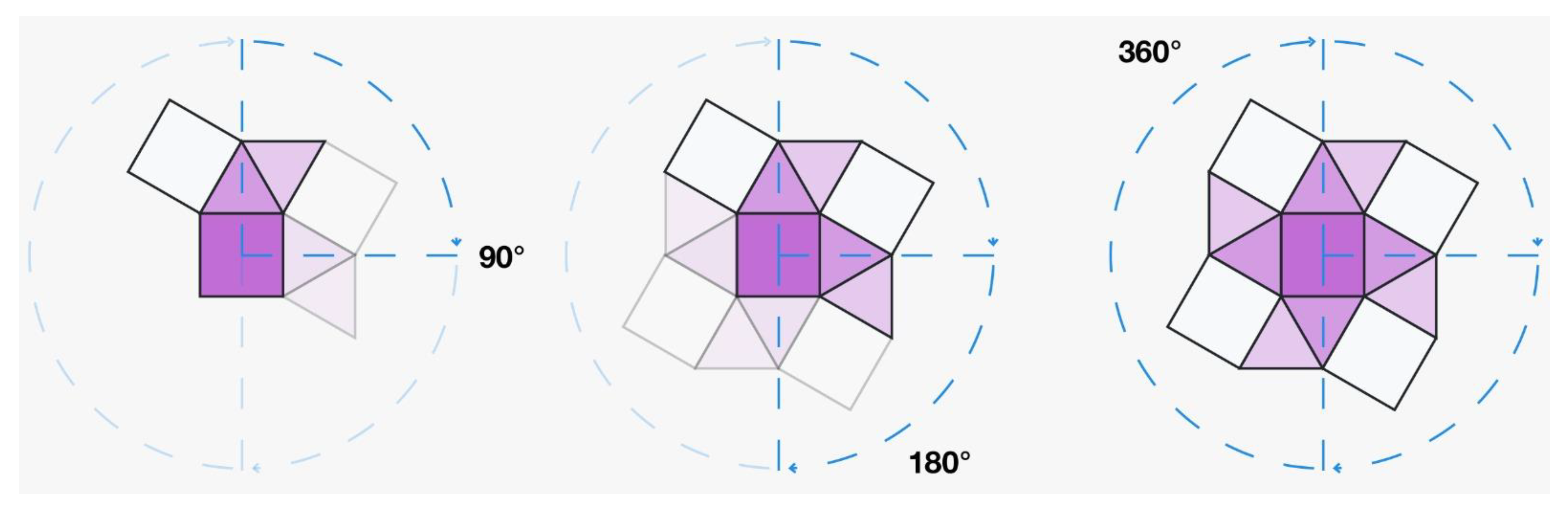
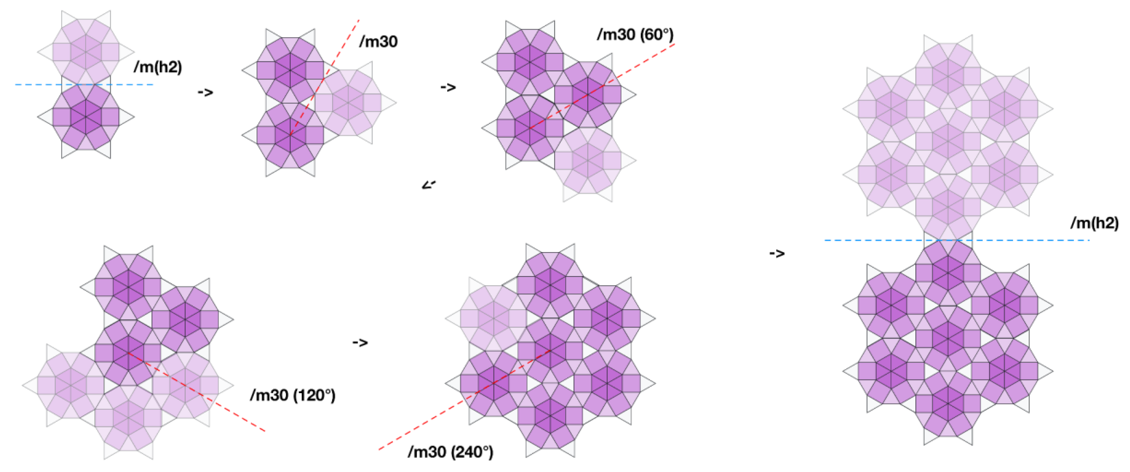
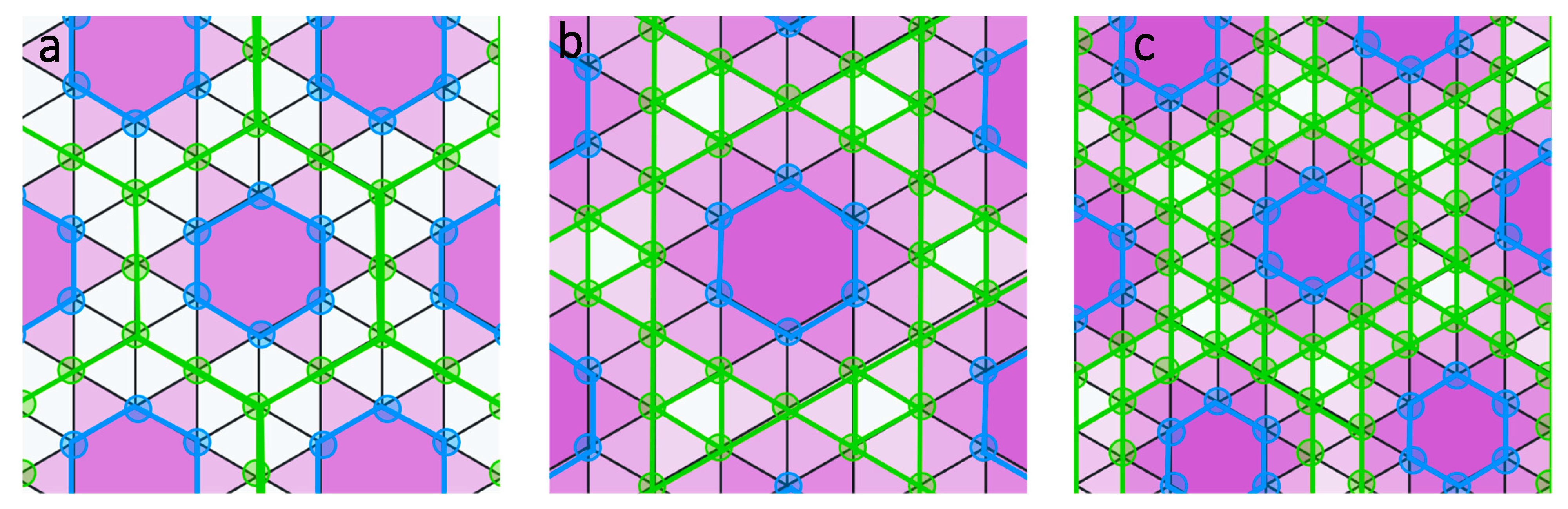
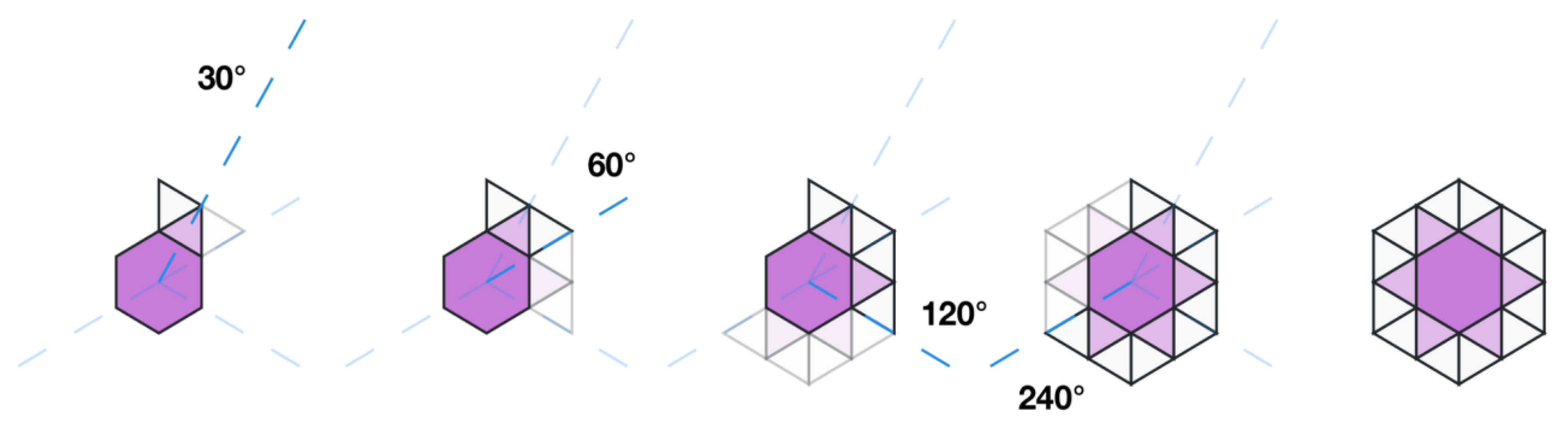
  • m30: Type of transform: m for mirroring. Angle 30°. An origin is not specified between parentheses, therefore the origin is the center of the coordinate system. Therefore this transform is going to reflect by 30° the elements of the previous phase obtained in Figure 6 along an axis passing by the center of the coordinate system.
  • Then, it reflects 60° (30° × 2) the result of the previous transformation.
  • Reflect 120° (60° × 2) the result of the previous transformation.
  • Reflect 240° (120° × 2) the result of the previous transformation. This is the last reflection as 240° × 2 is 480° and is above the 360° limit.
Figure 9 shows another example (4-3-4,3/r90) where, instead of mirroring, a transformation has been applied by means of a series of rotations.

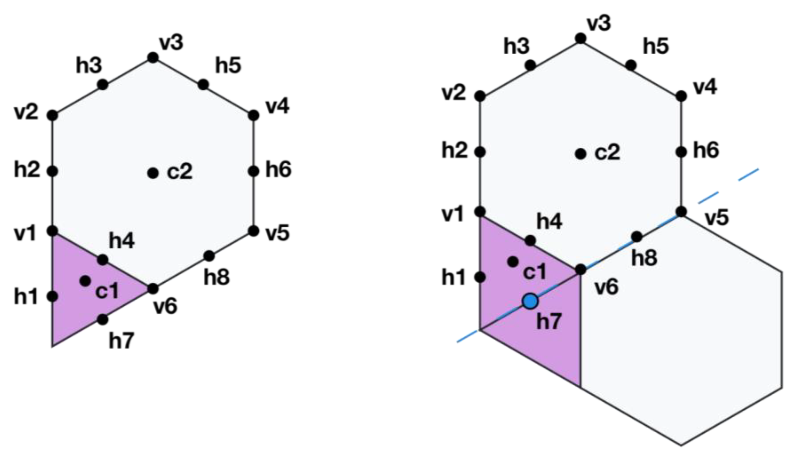
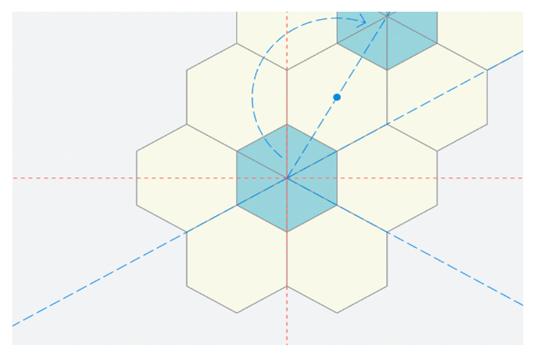
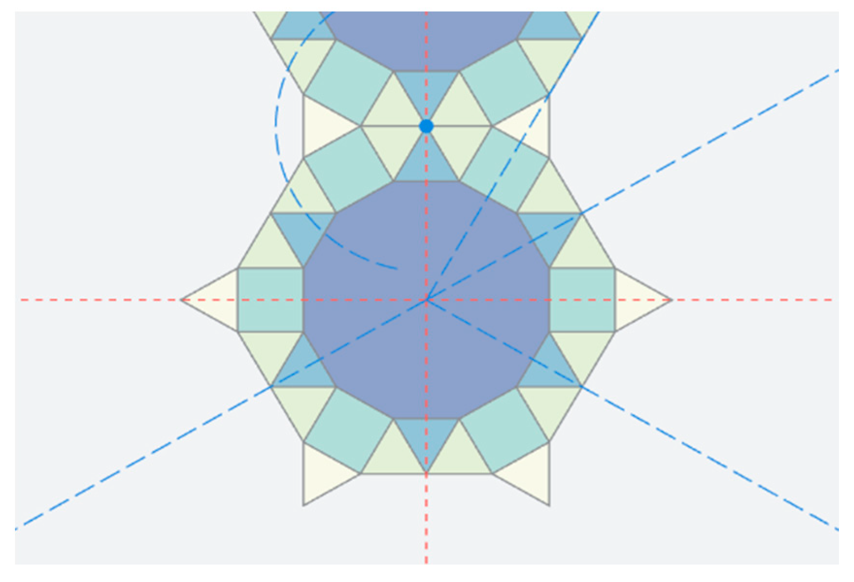
3.2.2. Origin 2. Points on the Polygons—Eccentric Transformation

There will always be a need for two or more transforms to completely cover a plane. At least one of these transform functions will need to shift the transform’s origin from the center of the coordinate system in order to expand the collection of shapes out to increase the area coverage. This is done by shifting the transform’s origin to either the vertex of a polygon, the centroid of a polygon or a midpoint of a line segment.
Unlike when the transform’s origin is at the center of the plane, transforms with its origin elsewhere are not continuous. In other words, they are performed only once before moving onto the next transform.
The notation for shifting the transform’s origin is done by specifying the vertex index. The vertices available for a transform are systematically indexed prior to the transformation and are grouped by their vertex type and ordered by their distance and angle, relative to the center of the coordinate system. Polygon centroids are prefixed with a ‘c’, vertices of a polygon are prefixed with a ‘v’ and line halfway points are prefixed with an ‘h’.
Taking the configuration 3–6 (Figure 10, left), there are 16 possible origins in total, made up of 2 shape centroids (c1 to c2), 6 polygon vertices (v1 to v6) and 8 line segment halfway points (h1 to h8). Excluding the coordinate system center vertex.
Starting at 0° of the coordinate system, there are 4 vertices that exist at this angle, labelled h1, v1, h2 and v2 in order of the shortest distance to the origin. Moving clockwise, they are followed by vertex h3 which is next in turn by angle to the origin, and so on. As an example it would then be possible to reflect over the 1st vertex by specifying m(h7) in the notation (Figure 10, right), and the vertices would be reindexed for the next transformation function.
When specifying the vertex of a polygon’s centroid (Figure 11) or vertex (Figure 12), the angle that is used for the transformation is inferred from the angle of that vertex relative to the center of the coordinate system. However, when using the midpoint of a line segment (the polygon’s edge, as shown in Figure 10, right), the angle for the transform is inferred from the angle of that edge because any other angle would result in an incorrect overlapping and an invalid tessellation.

3.3. Stage 3: Repeating the Transformations

This is the final stage to completing the tiling, which consists of continuously repeating over the transforms in order, indefinitely (Figure 13). For notations that are valid, the tessellation would continue to grow, increasing in surface area. Shapes being reflected into the exact position of an existing shape are merged, however valid notations should not result in any gaps or intersecting shapes—as shown in Figure 14.

4. ANTWERP, the Software

The notation presented above has been thoroughly proved by means of the software “ANTWERP: Application for Nets and Tessellations with Edge-to-edge Regular Polygons”, in its version v3.0 [5]. ANTWERP is a free online application, which is publicly shared to prove that all the basic tilings can be obtained directly from the GomJau-Hogg’s notation. It lets the user automatically generate all of the existing regular and semi-regular tilings as well as the demi-regular tilings. The latter are also called k-uniform.
The first version of this application (v1.0) was originally coded with Visual Basic for Application (VBA) applied to AutoCad. The main problem was that users without Autocad could not exploit the program. In its second version, ANTWERP v2.0 was accessible over a network connection using HTTP; therefore the program could be run from any PC, tablet, phone, etc. on a web browser that supported WebGL (over JavaScript).
The current version, ANTWERP v3.0, uses an updated version of the notation, from that presented previously [3], with greater flexibility to generate the more complex tessellations. It is a TypeScript React application, with a custom tessellation renderer that has been published as a package (available online: https://www.npmjs.com/package/@hhogg/antwerp, accessed on 29 October 2021) to produce SVGs from the notation. This package can be imported into any Web Application that takes this notation (plus some optional configuration) and renders a downloadable SVG file.

5. Results

One of the main results is the production of Table 1 and Appendix A, which show the translation from Cundy & Rollett’s notation to GomJau-Hogg’s notation for the most basic tilings, in such a way that if solves the two main problems of Cundy & Rollett’s notation:
  • The notation of the tilings can be automatically generated without ambiguity
  • There is no repetition on the names of the tilings, they are unique.
Table 1 and Appendix A list only the k-uniform tessellations for k < 4. More complex tilings can be named and generated with GomJau-Hogg’s notation, but the list is longer and longer as k increases. According to Galebach [6], the number of tilings for k = 1 is 11, for k = 2 is 20, for k = 3 is 61, for k = 4 is 151, for k = 5 is 332 and for k = 6 is 673. For higher k > 6 the number of existing tilings is still unknown but very high. The current version of this software does not convert the older notation into the new one. The process that we have followed is to find, one by one, the notation that would create each one of the k-uniform tilings for k < 4. It is a time-consuming process that should be improved in order to find and generate all the existing k-uniform tessellations.

6. Conclusions and Further Research

As a conclusion, this work presents a method for generating all the regular, uniform and k-uniform (up to at least k = 3) in a consistent, unique and unequivocal manner by means of a new notation applied to a new software (ANTWERP v3.0). Further communications will prove that it is possible to deduct automatically, from our notation, to which group of wallpaper symmetry each tessellation belongs.

Building an Exhaustive Tessellation Database

In further research, we plan to use computing resources to continuously iterate through the permutations of this notation to build an exhaustive database of possible tessellations. This will be done by representing the tessellation notation as a tree data structure, traversing it to find the paths that lead to an infinitely repeating tessellation (Figure 15) and optimizing by removing paths that lead to invalid tessellations that either do not expand or cause overlaps (Figure 16).
Using this tree data structure approach and a breadth-first-search algorithm, we will also be able to improve on our current findings by identifying the most optimal notations to represent tessellations. For example, 4-3,3,3-4,3/r(c2)/r(h13)/r(h45) which uses 3 transformations, was manually created by us to construct the tessellation, however this algorithmic approach might discover a notation to do it in just 2 transformations. Part of this, will require a method to perform comparisons on generated tessellations (for example, through pattern recognition machine learning [7]) that have been produced with different structures but ultimately lead to the same output (Figure 17).
All these findings can be applied to many fields of engineering where tilings have a major importance in design configurations (mechanical, civil, chemical, etc.).

Author Contributions

Conceptualization, V.G.-J. and H.H.; methodology, C.O. and C.M.; software, H.H.; investigation, V.G.-J.; writing—original draft preparation, V.G.-J. and H.H; writing—review and editing, V.G.-J., H.H., C.O. and C.M. All authors have read and agreed to the published version of the manuscript.

Funding

This research received no external funding.

Institutional Review Board Statement

Not applicable.

Informed Consent Statement

Not applicable.

Data Availability Statement

https://antwerp.hogg.io/library (accessed on 29 October 2021).

Conflicts of Interest

The authors declare no conflict of interest.

Appendix A

Appendix A shows an array of figures representing graphically all the tilings gathered in Table A1 with both notations.
Table A1. Array of figures representing graphically all the tilings gathered in this table with both notations.
Symmetry 13 02376 i001
Symmetry 13 02376 i002
Symmetry 13 02376 i003
Symmetry 13 02376 i004
Symmetry 13 02376 i005
Symmetry 13 02376 i006
Symmetry 13 02376 i007

References

  1. Otero, C. Diseño Geométrico de Cúpulas No Esféricas Aproximadas por Mallas Triangulares con un Número Mínimo de Longitudes de Barra. Ph.D. Thesis, University of Cantabria, Santander, Spain, 1990. [Google Scholar]
  2. Cundy, H.M.; Rollett, A.P. Mathematical Models; Tarquin Publications: Stradbroke, UK, 1981. [Google Scholar]
  3. Gomez-Jauregui, V.; Otero, C.; Arias, R.; Manchado, C. Generation and Nomenclature of Tessellations and Double-Layer Grids. J. Struct. Eng. 2012, 138, 843–852. [Google Scholar] [CrossRef]
  4. Grünbaum, B.; Shephard, G.C. Tilings and Patterns; W. H. Freeman & Co.: New York, NY, USA, 1986. [Google Scholar]
  5. Hogg, H.; Gomez-Jauregui, V. Antwerp v3.0.0. 2019. Available online: https://antwerp.hogg.io (accessed on 17 October 2021).
  6. Galebach, B.L. Number of N-Uniform Tilings. 2003. Available online: https://www.probabilitysports.com/tilings.html (accessed on 30 November 2021).
  7. Khan, A.A.; Laghari, A.A.; Awan, S.A. Machine Learning in Computer Vision: A Review. EAI Endorsed Trans. Scalable Inf. Syst. 2021, 8. [Google Scholar] [CrossRef]
Figure 1. Regular tilings: (a) 36, (b) 63 and (c) 44.
Symmetry 13 02376 g001
Figure 2. Semi-regular tilings, 3 examples: (a) 3.12², (b) 3.4.6.4 and (c) 4.6.12.
Symmetry 13 02376 g002
Figure 3. Demi-regular tilings, 3 examples: (a) 36; 32.4.3.4, (b) 3.4.6.4; 32.4.3.4 and (c) 3.4.6.4; 3.42.6.
Symmetry 13 02376 g003
Figure 4. Vertices (a) 36 in yellow, (b) 36 in green and (c) 34.6 (in blue), being (a,b) of different transitivity class, along with the composition of one of the three different tessellations with the same vertex notation: (36)2; 34.6.
Symmetry 13 02376 g004
Figure 5. Three different tessellations with the same Cundy & Rollett nomenclature: (a) [(36)2; 34.6]1; (b) [(36)2; 34.6]2 and (c) [(36)2; 34.6]3. In green, vertices (36), in blue, vertices 34.6. Their configuration is different for the three of them.
Symmetry 13 02376 g005
Figure 6. Equation formatting: 6-3-3.
Symmetry 13 02376 g006
Figure 7. Seed polygons of 3, 4, 6, 8 and 12.
Symmetry 13 02376 g007
Figure 8. Continuous centered transformation (Mirroring): Example of 6-3-3/m30 with center in the origin of coordinate system.
Symmetry 13 02376 g008
Figure 9. Continuous centered transformation (Rotation): Example of 4-3-4,3/r90 with center in the origin of coordinate system.
Symmetry 13 02376 g009
Figure 10. Eccentric transformation (Mirroring): Example of 3-6/m(h7) with center in point h7 (seventh halfway point).
Symmetry 13 02376 g010
Figure 11. Equation formatting 3-6/m30/r(c2).
Symmetry 13 02376 g011
Figure 12. Equation formation 12-3,4-3,3/m30/r(v1).
Symmetry 13 02376 g012
Figure 13. Repeated transforms /m(h2) → /m30* → /m(h2).
Symmetry 13 02376 g013
Figure 14. Equation formatting 4-3-3-0,4/r90/r(h3).
Symmetry 13 02376 g014
Figure 15. Tree data structure representation of the valid notation 3-4-3,3/m30/m(h2).
Symmetry 13 02376 g015
Figure 16. Tree data structure representation of an invalid notation 3-12,6. Invalid due to the angle of the empty space between the hexagon and the dodecagon.
Symmetry 13 02376 g016
Figure 17. The same tessellation pattern but with different notations: (a) 4-4,4-3,4-6/m90/r(c5)/r(v1) and (b) 6-3,4-0,4,4-0,4/m90/m90(c5)/m(v1).
Symmetry 13 02376 g017
Table 1. Transformation of Cundy & Rollett’s notation to GomJau-Hogg’s notation, up to 3-Uniform (3 Vertex Types). All of these can be seen in the tilings explorer application of Antwerp https://antwerp.hogg.io/library (accessed on 29 October 2021).
CUNDY & ROLLETTGOMJAU-HOGG
REGULAR
363/m30/r(h2)
636/m30/r(h1)
444/m45/r(h1)
UNIFORM
3.12212-3/m30/r(h3)
3.4.6.46-4-3/m30/r(c2)
4.6.1212-6,4/m30/r(c2)
(3.6)26-3-6/m30/r(v4)
4.828-4/m90/r(h4)
32.4.3.44-3-3,4/r90/r(h2)
33.424-3/m90/r(h2)
34.66-3-3/r60/r(h5)
2 UNIFORM
36; 32.4.3.43-4-3/m30/r(c3)
3.4.6.4; 32.4.3.46-4-3,3/m30/r(h1)
3.4.6.5; 33.426-4-3-3/m30/r(h5)
3.4.6.4; 3.42.66-4-3,4-6/m30/r(c4)
4.6.12; 3.4.6.412-4,6-3/m30/r(c3)
36; 32.4.1212-3,4-3/m30/r(c3)
3.122; 3.4.3.1212-0,3,3-0,4/m45/m(h1)
36; 32.623-6/m30/r(c2)
[36; 34.6]16-3,3-3/m30/r(h1)
[36; 34.6]26-3-3,3-3/r60/r(h8)
32.62; 34.66-3/m90/r(h1)
3.6.3.6; 32.626-3,6/m90/r(h3)
[3.42.6; 3.6.3.6]16-3,4-6-3,4-6,4/m90/r(c6)
[3.42.6; 3.6.3.6]26-3,4/m90/r(h4)
[33.42; 32.4.3.4]14-3,3-4,3/r90/m(h3)
[33.42; 32.4.3.4]24-3,3,3-4,3/r(c2)/r(h13)/r(h45)
[44; 33.42]14-3/m(h4)/m(h3)/r(h2)
[44; 33.42]24-4-3-3/m90/r(h3)
[36; 33.42]14-3,4-3,3/m90/r(h3)
[36; 33.42]24-3-3-3/m90/r(h7)/r(h5)
3-UNIFORM (2 VERTEX TYPES)
(3.4.6.4)2; 3.42.66-4-3,4-6,3/m30/r(c2)
[(36)2; 34.6]16-3-3/m30/r(v3)
[(36)2; 34.6]26-3-3-3-0,3/m30/r(v2)
[(36)2; 34.6]36-3-3,3-3-3-0,3/r60/r(h7)
36; (34.6)23-3,3-6/m90/r(h6)
36; (32.4.3.4)23-4-3,3/m30/m(h2)
(3.42.6)2; 3.6.3.64-6,4-4,3,3/m90/r(h4)
[3.42.6; (3.6.3.6)2]14-6,4-0,3,3/m/r(v1)/r(h25)
[3.42.6; (3.6.3.6)2]24-6,4-0,3,3/m90/r(v1)
32.62; (3.6.3.6)26-3,0,3,3,3,3/r(h4)/r(v15)/r(v30)
(34.6)2; 3.6.3.66-3,3-0,3/r/r(v1)/r(h12)
[33.42; (44)2]14-4-4-3/m90/r(h4)
[33.42; (44)2]24-4-3/r(h6)/m(h5)/r(h3)
[(33.42)2; 44]14-4-3-3-4/m90/r(h10)/r(c3)
[(33.4²)2; 44]24-3,4-3,3-4/m90/r(h3)
(33.42)2; 32.4.3.44-4,3,4-3,3,3-3,4-3-4/r/r(h17)/r(h18)
33.42; (32.4.3.4)24-3,3-0,4,3/r/r(h2)/r(h18)
[36; (33.42)2]14-3,0,3-3-3/r(h5)/r(h19)/m(h18)
[36; (33.42)2]24-3,0,3-3/r(h3)/r(h15)/m(h14)
[(36)2; 33.42]14-3-3-3-3-3/m90/r(h3)
[(36)2; 33.42]24-3-3-3-3/m90/r(h2)/m(h22)
3-UNIFORM (3 VERTEX TYPES)
3.42.6; 3.6.3.6; 4.6.1212-6,4-3,3,4/m30/r(c5)
3⁶; 32.4.12; 4.6.1212-3,4,6-3/m60/m(c5)
32.4.12; 3.4.6.4; 3.1226-4-3,12,3-3/m30/r(h2)
3.4.3.12; 3.4.6.4; 3.1226-4-3,3-12-0,0,0,3/m30/r(c2)
33.42; 32.4.12; 3.4.6.412-4,3-6,3-0,0,4/m30/r(h11)
3⁶; 33.42; 32.4.1212-3,4-3-3-3/m30/m(h9)
36; 32.4.3.4; 32.4.1212-3,4-3,3/m30/r(v1)
34.6; 33.42; 32.4.3.46-3-3-4-3,3/m30/r(h10)
36; 32.4.3.4; 3.42.63-4-3,4-6/m30/r(c5)
36; 33.42; 3.4.6.46-4-3,4-3,3/m30/r(c5)
36; 32.4.3.4; 3.4.6.46-4-3,3-4,3,3-3/r60/r(v5)
36; 33.42; 32.4.3.43-4-3-3/m30/r(h6)
32.4.12; 3.4.3.12; 3.12212-4-3,3/m90/r(h6)
3.4.6.4; 3.42.6; 446-4,3-3,0,4-6/m90/r(v5)
32.4.3.4; 3.4.6.4; 3.42.66-4,3-3,3,4-0,0,6,3/m90/r(h17)/m(h1)
33.42; 32.4.3.4; 444-3-3-0,4/r90/r(h3)
[3.42.6; 3.6.3.6; 44]14-4-3,4-6/m/r(c3)/r(h29)
[3.42.6; 3.6.3.6; 44]24-4,4-3,4-6/m90/r(c5)/r(v1)
[3.42.6; 3.6.3.6; 44]36-3,4-0,4,4-0,4/m90/r(h9)
[3.42.6; 3.6.3.6; 44]46-4,3,3-4/m(h4)/r/r(v15)
33.42; 32.62; 3.42.64-6-3,0,3,3-0,0,4/m90/r(h4)
[32.62; 3.42.6; 3.6.3.6]14-6,4,3-0,3,3,0,6/m(h2)/m
[32.62; 3.42.6; 3.6.3.6]24-6,4-0,3,3/r(h2)/m90/r(c9)
34.6; 33.42; 3.42.64-6,4-0,3,3-0,3,3/r/r(c1)/r(h17)
[32.62; 3.6.3.6; 63]16-6-3,3,3/r60/r(h2)
[32.62; 3.6.3.6; 63]26-6,6,3-3,3/m//r(h8)/r(h49)
34.6; 32.62; 636-3-3/m/r(h3)/r(h15)
36; 32.6²; 633-6/r60/m(c2)
[36; 34.6; 32.62]16-3-3,3-3,3-0,3/r(h7)/r(h29)/r(h29)
[36; 34.6; 32.62]23-3,6-3/m/r(h6)/r(c6)
[36; 34.6; 32.62]36-3-3/m90/r(h2)
[36; 34.6; 3.6.3.6]13-3,3-3,6,3/m90/r(v1)/r(v15)
[36; 34.6; 3.6.3.6]23-3-6-0,3/r60/m(c1)
[36; 34.6; 3.6.3.6]33-3-6/r60/r(v4)
[36; 33.42; 44]14-4-3-3/m90/r(h7)/r(v1)
[36; 33.4²; 44]24-4-3-3-3/m90/r(h9)/r(h3)
[36; 33.42; 44]34-4-3-3-3/m(h9)/r(h1)/r(v1)
[36; 33.42; 44]44-4-3-3-3/m(h9)/r(h1)/r(h3)
Publisher’s Note: MDPI stays neutral with regard to jurisdictional claims in published maps and institutional affiliations.

