Abstract
Finding defects early in a software system is a crucial task, as it creates adequate time for fixing such defects using available resources. Strategies such as symmetric testing have proven useful; however, its inability in differentiating incorrect implementations from correct ones is a drawback. Software defect prediction (SDP) is another feasible method that can be used for detecting defects early. Additionally, high dimensionality, a data quality problem, has a detrimental effect on the predictive capability of SDP models. Feature selection (FS) has been used as a feasible solution for solving the high dimensionality issue in SDP. According to current literature, the two basic forms of FS approaches are filter-based feature selection (FFS) and wrapper-based feature selection (WFS). Between the two, WFS approaches have been deemed to be superior. However, WFS methods have a high computational cost due to the unknown number of executions available for feature subset search, evaluation, and selection. This characteristic of WFS often leads to overfitting of classifier models due to its easy trapping in local maxima. The trapping of the WFS subset evaluator in local maxima can be overcome by using an effective search method in the evaluator process. Hence, this study proposes an enhanced WFS method that dynamically and iteratively selects features. The proposed enhanced WFS (EWFS) method is based on incrementally selecting features while considering previously selected features in its search space. The novelty of EWFS is based on the enhancement of the subset evaluation process of WFS methods by deploying a dynamic re-ranking strategy that iteratively selects germane features with a low subset evaluation cycle while not compromising the prediction performance of the ensuing model. For evaluation, EWFS was deployed with Decision Tree (DT) and Naïve Bayes classifiers on software defect datasets with varying granularities. The experimental findings revealed that EWFS outperformed existing metaheuristics and sequential search-based WFS approaches established in this work. Additionally, EWFS selected fewer features with less computational time as compared with existing metaheuristics and sequential search-based WFS methods.
1. Introduction
The software development lifecycle (SDLC) is a formal framework that has been specifically planned and built for the production or development of high-quality software systems. To ensure a timely and reliable software system, the SDLC incorporates gradual steps such as requirement elicitation, software system review, software system design, and software system maintenance, which must be carefully followed and applied [1,2,3]. However, since the SDLC step-by-step operations are done by human professionals, failures are inevitable. Because of the large scale and dependencies in modules or parts of software systems today, these errors are common and recurring. If not corrected immediately, these errors will result in unreliable computing structures and, ultimately, software failure. That is, the occurrence of errors in information system modules or components will result in flawed and low-quality software systems. Furthermore, vulnerabilities in software systems can irritate end-users and customers when the failed software system does not work as expected after having wasted scarce resources (time and effort) [4,5,6,7]. Hence, it is important to consider early prediction and recognition of software flaws before product delivery or during the software development processes. Early detection or prediction of incorrect (defective) modules or components in a software system allows those modules or components to be automatically corrected and available resources to be used wisely [8,9].
At the unit level, testing critical source codes necessitates selecting test data from the input domain, running the source codes with the selected test data, and checking the accuracy of the computed outputs [3]. The symmetric testing strategy is an applicable example. Symmetric testing tries to test source code that does not require an oracle or any formal specification. The permutation relations between source code runs are typically used to automate the testing process. Primarily, symmetric testing uses a combination of automated test data production and symmetries, checking to identify flaws or vulnerabilities in a software system [10]. However, one disadvantage of automated testing methodologies is the difficulty in designing and troubleshooting automated test scripts [11]. Another viable approach is the use of machine learning (ML) methods to determine the defectivity of modules or components in a software system. This approach is known as software defect prediction (SDP). Specifically, SDP is the application of ML methods to software features identified by software metrics to identify faults in software modules or components [12,13,14,15]. Several researchers have suggested and applied both supervised and unsupervised ML approaches for SDP [16,17,18,19,20,21].
Nonetheless, the predictive accuracy of SDP models is entirely dependent on the consistency and inherent design of the software datasets used in their creation. The magnitude and complexities of information systems are closely related to the software metrics used to characterize the consistency and performance of software systems. To put it another way, large and scalable software systems necessitate many software metric structures to deliver functionality that best reflects the output of those software systems [22,23]. In general, software systems with many features are composed of redundant and insignificant features, resulting from the accumulation of software metrics. This can be described as a high dimensionality problem. Several studies have shown that the high dimensionality of software metrics has a negative effect on the predictive performance of SDP models [24,25]. Researchers agree that the feature selection (FS) approach is an effective method for addressing high-dimensionality problems [26,27,28,29]. For each SDP operation, these FS methods essentially extract valuable and critical software features from the initial software defect dataset [27,28,30].
The implementation of FS methods will lead to the formation of a subset of features that contains germane and crucial features from a set of irrelevant and excessive features, thus overcoming the high dimensionality of the dataset. The application of FS methods results in the creation of a subset of features containing germane and critical features from a collection of trivial and unnecessary features, thus resolving the dataset’s high dimensionality. In other words, FS methods select important features while retaining dataset accuracy. Finally, this solves the issue of the high dimensionality of software defect datasets. FS methods select prominent features while ensuring the quality of the dataset. In the end, this solves the high dimensionality problem of software defect datasets [30,31]. There are two types of FS methods: filter feature selection (FFS), and wrapper feature selection (WFS). FFS approaches test dataset attributes by using the dataset’s underlying computational or predictive properties. Following that, the top-ranked features are selected depending on the predefined threshold score. In contrast to FSS, WFS methods test dataset functionality based on their usefulness in improving the efficiency of underlining classifiers. In other words, WFS chooses features based on classifier results.
However, there are still notable issues with WFS methods. The process of subsets generation in WFS methods largely depends on the search strategy used. A key problem with WFS is how to search into the space of feature subsets. Using an exhaustive search strategy leads to high time complexity, since all possible feature subsets are considered, while a heuristic search strategy does not consider all possible feature subsets, being a stochastic process [28,32,33,34,35]. While several WFS methods based on metaheuristic and sequential searches have been proposed and developed, the local maxima stagnation problem and high computational costs due to large search space persist [30,31,32,33,36]. WFS approaches have been recognized to have significant computational costs, since the number of executions necessary for feature subset search, assessment, and selection are unknown in advance, which often leads to overfitting of prediction models owing to easy entrapment in local maxima. In the WFS subset evaluator phase, using the right search technique may resolve its entrapment in local maxima.
In addition, finding a way to reduce the evaluation time of WFS, that is, computational cost, while maintaining its performance, is imperative. As a result, this study proposes a novel re-ranking strategy-based WFS method to dynamically and iteratively select features. The proposed enhanced WFS (EWFS) method is based on incrementally selecting features while considering previously selected features in its search space.
The main contributions of this study are as follows:
- An enhanced wrapper feature selection (EWFS) method based on a dynamic re-ranking strategy was developed.
- The performance of the proposed EWFS was evaluated and compared with existing sequential and metaheuristic search-based WFS methods.
- The effectiveness of EWFS as a solution for high dimensionality in SDP was validated.
The remainder of this paper is structured as follows: Reviews on existing related works are presented in Section 2. Details on proposed EWFS and experimental methods are described in Section 3. Experimental results are analyzed and discussed in Section 4, and the research is concluded with highlights of future work in Section 5.
2. Related Works
High dimensionality is a well-known data quality issue that typically harms the predictive capabilities of SDP models. In other words, a wide range of technological features or metrics affects the predictive performance of SDP models. FS methods are used to resolve high dimensionality as a data preprocessing activity by choosing appropriate and irredundant features. In this case, SDP is no exception, and many FS approaches have been used to improve the predictive performance of SDP models.
Wahono, et al. [37] used a metaheuristic-based WFS approach to improve an ensemble-based SDP model. They integrated Particle Swarm Optimization (PSO) and Genetic Algorithm as search methods for the wrapper. Their experimental results showed that the applied WFS method enhanced the predictive performance of the ensemble method.
Specifically, a hybrid metaheuristic search method based on PSO and GA was deployed as a search mechanism in the proposed WFS method. Findings from their study indicated that the proposed WFS can improve the implemented ensemble method’s prediction accuracy. This observation indicates that metaheuristic search approaches may be equally as effective as conventional BFS or GSW techniques as search methods in WFS. However, the performance of metaheuristic search methods depends on their hyper-parameterization. That is, getting the right or appropriate parameters for the metaheuristic-based WFS method is a problem.
Similarly, Song, et al. [38] utilized two WFS approaches in their study: forward-selection and backwards-elimination. Based on their findings, they concluded that both types of WFS had a beneficial impact on SDP models, asserting that there is no discernible distinction between their respective performances. Moreover, their work seems to have a drawback in that it only uses forward selection and backward removal as methods of analysis. Other search approaches, such as metaheuristics, may be as efficient as, if not more efficient than, forward-selection and backwards-elimination in terms of finding relevant results.
Muthukumaran, et al. [39] performed a detailed empirical study on 16 defect datasets using 10 diverse FS techniques. In their analysis, WFS founded on greedy stepwise search (GSS) methods outperformed other FS methods. Rodríguez, et al. [40] studied the impact of FS methods on prediction models in SDP. Particularly, they compared the effectiveness of correlation-based FS (CFS), consistency-based FS (CNS), fast correlation-based filter (FCBF), and WFS methods. The researchers claimed that selecting fewer features from datasets has greater prediction capabilities than the original dataset, and that the WFS approach outperforms the other tested FFS approaches. WFS approaches, on the other hand, are computationally expensive, perhaps as a result of relying on classical exhaustive search techniques. Moreover, testing the chosen features against a different base classifier does not ensure optimality.
Cynthia, et al. [41] looked into how FS methods affected SDP prediction models. The impact of five FS approaches on a set of classifiers was studied. From their results, they deduced that the prediction output of the selected classifiers was impacted (positively) by experimented FS methods. Despite this, the scope of their study (the number of FS methods and datasets used) was limited. Akintola, Balogun, Lafenwa-Balogun and Mojeed [2] investigated filter-based FS techniques on heterogeneous prediction models, focusing on principal component analysis (PCA), correlation-based feature selection (CFS), and filtered subset evaluation classifiers (FSE). They also observed that utilizing FS techniques in SDP is useful since it improves the prediction accuracy of selected classifiers.
Balogun, Basri, Jadid, Mahamad, Al-momani, Bajeh and Alazzawi [26] studied the performance of the WFS technique using several feature search methods. The effectiveness of 13 metaheuristics and 2 sequential search-based WFS systems was specifically examined. According to their experimental observations, WFS based on metaheuristic search approaches beat sequential search-based WFS methods in the majority of conducted experiments. Similarly, Mabayoje, et al. [42] investigated the effect of different WFS methods on prediction performances of SDP models. According to their findings, using WFS approaches may improve the accuracy of SDP model predictions. Furthermore, Ding [43], in their study, applied a GA as a search method in WFS to enhance the prediction performance of an isolation forest classifier (IFC). Findings from their results revealed the effectiveness of the proposed WFS method on implemented IFC. Yet, the computing time of metaheuristic search-based WFS techniques, on the other hand, was rather significant. This can be attributed to the easy trapping of metaheuristic search-based methods in local maxima and its convergence uncertainty.
Overall, WFS techniques are quite effective in reducing the number of data characteristics while simultaneously improving the prediction model’s performance. Despite this, the downsides of easily falling into local maxima and large computing costs continue to crop up. Consequently, this study proposes an EWFS method based on a dynamic re-ranking strategy to select relevant and irredundant features in SDP. Specifically, an entropy measure (in this case, Information Gain) is used to rank features, and then the ranked features are passed through an incremental wrapper method using conditional mutual information maximization (CMIM) while considering the initially selected features. CMIM balances and selects features by maximizing their respective mutual information with the class label while minimizing the co-dependency that may exist between or amongst features using a Multi-Objective Cuckoo search method. This process will reduce the number of wrapper evaluations, as only a few features are considered during each iteration while maintaining or amplifying the prediction performance of the selected features.
3. Methodology
This section presents and discusses the implemented classification algorithms, the proposed EWFS approach, experimented datasets, performance assessment measures, and experimental procedures.
3.1. Classification Algorithm
Decision Tree (DT) and Naive Bayes (NB) algorithms were chosen and used as prediction models in this analysis. The two were chosen because of their high prediction efficiency and potential to deal with imbalanced datasets [34,44]. In addition, parameter tuning seldom affects DT and NB. Furthermore, DT and NB have been used extensively in previous SDP reports. Details on implemented DT and NB classifiers are presented in Table 1.

Table 1.
Selected prediction models.
3.2. Enhanced Wrapper Feature Selection Method (EWFS) Based on Dynamic Re-Ranking Strategy
The proposed EWFS method is based on incrementally selecting features while considering previously selected features in its search space. First, an entropy measure is used to rank features from a dataset, and then the ranked features are passed through an incremental wrapper method. However, it is only the first B ranked feature selected by the entropy-based on that is passed to the incremental wrapper method. The use of features is per existing empirical studies in SDP [25,27,28]. Thereafter, the remaining features in B are re-ranked using conditional mutual information maximization (CMIM) (see Function 1) while considering the initially selected features. CMIM balances and selects features by maximizing their respective mutual information with the class label while minimizing the co-dependency that may exist between or amongst features using a Multi-Objective Cuckoo search method (see Function 2). In particular, CMIM attempts to balance the quantity of information provided for each possible attribute and class , as well as the possibility that this information has already been captured by some feature . As a result, this technique picks characteristics based on their mutual information with the class while reducing pair-to-pair dependence. For instance, given subset and a subset of features , the merit , i = 1, …, n is computed as = .
Then, the incremental wrapper method is applied to the newly ranked list after having been initialized by the first selected features from B. This process is repeated until there are no changes in the selected features. This process will reduce the number of wrapper evaluations, as only a few features are considered during each iteration while maintaining or amplifying the prediction performance of the selected features. Algorithm 1 shows the pseudocode for the proposed EWFS method.
| Algorithm 1 Pseudocode of proposed Enhanced WFS (EWFS) |
| Input: D: Dataset C: Classifier = |NB, DT| // to be used for subset evaluation in WFS E: Entropy Measure = |IG| // to be used for subset evaluation in WFS T: Threshold = log2n B: Block Size A = {0 ≤ B ≤ T}, N: Number of features CS: Multi-Objective Cuckoo Search Method Output: Subset of Optimal Features 1. for each { do 2. Rank = 3. R[ ] = } // assign ranked features in ascending order into R 4. 5. 6. .// select top-ranked features in R as the first block 7. 8. continue =: True 9. while (continue){ do 10. 11. for each { do 12. Rank = 13. } // assign ranked features in ascending order into R 14. 15. .// select top-ranked features in R as the first block 16. 17. if ( // append optimal features from based on T 18. continue =: False } 19. else 20. Return |
| Function 1 Pseudocode of Conditional Mutual Information Maximization (CMIM) [45] |
| Input: N: Number of features C: Class labels O: Initial set of features Output: Subset of Selected Features 1. for each { do 2. 3. 4. 5. for do 6. 7. for each { do 8. while do 9. 10. 11. If then 12. 13. 14. Return |
| Function 2 Pseudocode of Multi-Objective Cuckoo Search Method [46] |
| Initialize objective functions f1(x), …,fk(x);x = (x1, …xd)T Generate an initial population of n host nests xi and each with K eggs while (t < MaxGeneration) or (stop criterion) Get a cuckoo (say I) randomly by Levy flights Evaluate and check if it is Pareto optimal Choose a nest among n (say j) randomly Evaluate K solutions for nest j If new solutions of nest j dominate those of nest i, Replace nest i with the new solutions set of nest j End Abandon a fraction (po) of worse nests Keep the best solution s (or nest with non-dominated sets) Sort and find the current Pareto optimal solutions End |
3.3. Software Defect Datasets
This research employed defect datasets from four software repositories for experimentation. Specifically, twenty-five defect datasets were culled from PROMISE, NASA, AEEEM, and ReLink repositories. For the NASA repository, the Shepperd, et al. [47] version of defect datasets were selected in this research. The datasets consist of software properties produced by static code analysis. Static code analysis is derived from the source code size and complexity [25,27]. The PROMISE repository contains defect datasets derived from object-oriented metrics and additional information from software modules. This additional information is derived from Apache software [24,27,48]. Concerning the ReLink repository, datasets from this repository are derived from source code information taken from version control. These datasets were created by Wu, et al. [48] as linkage data, and these datasets have been frequently employed in previous SDP experimental studies [49,50,51]. Lastly, the AEEEM datasets comprise software features derived from software source code analysis that is dependent on software change metrics, entropy, and software code churn [25,27,39,48]. The description of these datasets is presented in Table 2.
Table 2.
Description of software defect datasets.
3.4. Experimental Procedure
In this section, details on the experimental procedure followed in this research as depicted in Figure 1 are described.
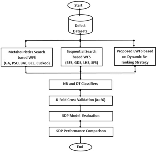
Figure 1.
Flowchart for the experimental procedure.
To evaluate the impact and effectiveness of the proposed EWFS on the predictive performance of SDP models, software defect datasets were used to construct SDP models based on NB and DT classification algorithms. Various scenarios were tested and investigated with non-biased and consistent performance comparative analyses of the resulting SDP models.
- Scenario A: In this case, the effectiveness of the proposed EWFS method is tested and correlated with the metaheuristic search-based WFS methods used in this study. The essence of this scenario is to evaluate and validate the performance of the EWFS against BAT, BEE, Genetic Algorithm (GA), Particle Swarm Optimization (PSO), and Cuckoo search-based WFS methods.
- Scenario B: In this scenario, the EWFS method’s performance is evaluated against sequential search-based WFS approaches as proposed in [52,53]. Findings from this scenario are used to validate the effectiveness of the proposed EWFS against Best First Search (BFS), GreeDy Step-Wise Search (GDS), Linear Forward Search (LFS), and Sequential Forward Search (SFS)-based WFS methods.
Experimental results and findings based on scenarios A and B are used to answer the following research questions.
- RQ1. How effective is the EWFS method in comparison to existing metaheuristic search-based WFS methods?
- RQ2. How effective is the EWFS method in comparison to existing sequential search-based WFS methods?
SDP models generated based on the above-listed scenarios are trained and tested using the 10-fold cross-validation (CV) technique. The CV technique guides against data variability issues that may occur in defect datasets. Moreover, the CV technique has been known to produce models with low bias and variance [54,55,56]. The prediction performances of generated SDP models are assessed using performance evaluation metrics such as accuracy, AUC, and f-measure. The Scott–Knott ESD statistical rank test is also used to ascertain the significant differences in the prediction performances of the various models studied. The Waikato Environment for Knowledge Analysis (WEKA) machine learning library [57], R programming language [58], and Origin Plot are used for the experimentation on an Intel(R) Core™ machine equipped with i7-6700, running at speed 3.4 GHz CPU with 16 GB RAM.
3.5. Performance Evaluation Assessment
In terms of performance evaluation, SDP models based on the proposed and other methods were analyzed using accuracy, the area under the curve (AUC), and f-measure values, metrics most often used in existing SDP studies to assess the performance of SDP models [9,59].
- i.
- Accuracy is the amount of data accurately estimated out of the actual number of data and can be represented as shown in Equation (1).
- ii.
- F-measure is computed based on the harmonic mean of precision and recall values of observed data. Equation (2) presents the formula for calculating the f-measure value.
- iii.
- The area under curve (AUC) signifies the trade-off between true positives and false positives. It demonstrates an aggregate output assessment across all possible classification thresholds.
, , TP = true positive (represents accurate prediction); FP = false positive (represents inaccurate prediction); TN = true negative (represents accurate mis-prediction); and FN = false negative (represents inaccurate mis-prediction).
4. Results and Discussion
In this section, findings from experiments concerning the experimental procedure as outlined in Section 3.4 are reported and discussed. Performance metrics such as accuracy, AUC, and f-measure values were used to test the predictive efficiency of NB and DT classifiers based on proposed EWFS, metaheuristic search-based WFS, and sequential search-based WFS. Table 3 presents the experimental results of the proposed EWFS method with NB and DT classifiers on twenty-five defect datasets based on the selected performance metrics. SDP models using EWFS on selected classifiers (NB and DT) were generated utilizing the 10-fold CV method and each experimental process was repeated 10 times. As depicted in Table 3, the proposed EWFS with NB and DT classifier had an average accuracy value of 82.57% and 83.07%, respectively, which shows that models (NB and DT) based on EWFS have a high chance of correctly predicting the average defects in SDP, which translates to a good prediction performance of models based on EWFS. Concerning AUC values, EWFS with NB and DT recorded average AUC values of 0.783 and 0.723, respectively. The high AUC values of models based on EWFS signifies that the prediction process is effective. In addition, the high average AUC values of EWFS on NB (0.768) and DT (0.708) further support its high accuracy value such that the developed models can identify defective and non-defective modules or components. Concerning the average f-measure value, the proposed EWFS had high average f-measure values on NB (0.807) and DT (0.820), which means that the models based on EWFS models have good precision and recall values. That is, the high f-measure of EWFS with NB and DT indicates that the developed models are precise and robust in identifying defective modules or components. Additionally, EWFS selects an average of five features at a relatively low average computational time of 3.318 s. This can be attributed to the dynamism of the re-ranking strategy which selects features iteratively and reduces the sunset search evaluation method without compromising the performance of the ensuing prediction model.
Table 3.
Analysis of experimental performance results of proposed EWFS method.
The experimental results analysis shows the applicability and performance of the proposed EWFS in selecting optimal features in a relatively low computational time without limiting its performance. The following sub-sections focus on the performance comparison of the proposed EWFS against existing metaheuristic search-based WFS and sequential search-based WFS. The essence of the comparison is to compare the performance of the proposed EWFS against existing WFS methods with different subset search approaches.
4.1. Comparison of Proposed EWFS Method against Metaheuristic Search-Based WFS Methods
In this sub-section, the performance of the proposed EWFS is compared with metaheuristic search-based WFS. Specifically, the prediction performance of NB and DT models based on the proposed EWFS and WFS based on Genetic Algorithm (GA), Particle Swarm Optimization (PSO), Bat Search (BAT), Bee Search (BEE), and Cuckoo Search (Cuckoo) are compared and contrasted.
Figure 2 presents box-plot representations based on average accuracy values of NB and DT models with EWFS and metaheuristic search-based WFS methods. In terms of average accuracy values, the proposed EWFS with NB and DT classifiers had superior average accuracy values when compared with NB and DT models based on the metaheuristic search-based WFS method. EWFS with NB and DT recorded average accuracy values of 82.57% and 83.07%, respectively, compared with the metaheuristic search-based WFS method based on GA (NB: 81.57%, DT: 81.58%), PSO (NB: 81.7%, DT: 81.55%), BAT (NB: 81.4%, DT: 81.64%), BEE (NB: 81.79%, DT: 81.9%), and Cuckoo (NB: 81.66%, DT: 81.84%). Specifically, NB and DT models based on EWFS outperformed models based on GA by +1.23% and +1.83%, PSO by +1.06% and +1.49%, BAT by +1.44% and +1.75%, BEE by +0.95% and +1.43%, and Cuckoo by +1.11% and +1.5%, respectively, based on average accuracy values. Thus, these analyses indicate the performance and superiority of EWFS over metaheuristic search-based WFS (GA, PSO, BAT, BEE, and Cuckoo) methods based on average accuracy values.
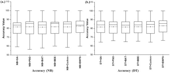
Figure 2.
Box-plot representations of the performance (accuracy) of EWFS and metaheuristic search-based WFS methods on NB and DT classifiers. (a) Average accuracy values of NB (b) Average accuracy values of DT.
Figure 3 presents the box-plot representations based on average AUC values of NB and DT models with EWFS and metaheuristic search-based WFS methods. NB and DT classifiers with the EWFS method recorded higher average AUC values when compared against models based on metaheuristic search-based WFS methods. EWFS with NB and DT recorded average AUC values of 0.768 and 0.708, respectively, compared with the metaheuristic search-based WFS method based on GA (NB: 0.739, DT: 0.683), PSO (NB: 0.722, DT: 0.683), BAT (NB: 0.722, DT: 0.68), BEE (NB: 0.728, DT: 0.683), and Cuckoo (NB: 0.725, DT: 0.686). In particular, NB and DT models based on EWFS outperformed models based on GA by +3.92% and +3.66%, PSO by +6.37% and +3.66%, BAT by +6.37% and +4.11%, BEE by +5.49% and +3.66%, and Cuckoo by +5.93% and +3.21%, respectively, based on average AUC values.
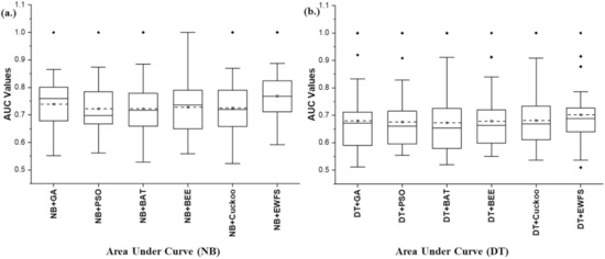
Figure 3.
Box-plot representations of the performance (AUC) of EWFS and metaheuristic search-based WFS methods on NB and DT classifiers. (a) Average AUC values of NB (b) Average AUC values of DT.
Additionally, Figure 4 shows box-plot representations based on average f-measure values of NB and DT models with EWFS and metaheuristic search-based WFS methods. Prediction models (NB and DT) with EWFS methods recorded average f-measure values of 0.821 and 0.826, respectively, which are superior to the average f-measure values of models based on metaheuristic search-based WFS methods such as GA (NB: 0.791, DT: 0.796), PSO (NB: 0.794, DT: 0.799), BAT (NB: 0.797, DT: 0.796), BEE (NB: 0.793, DT: 0.8), and Cuckoo (NB: 0.793, DT: 0.798).
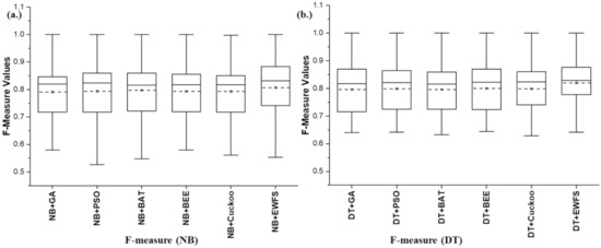
Figure 4.
Box-plot representations of the performance (f-measure) of EWFS and metaheuristic search-based WFS methods on NB and DT classifiers. (a) Average F-measure values of NB (b) Average F-measure values of DT.
Specifically, NB and DT models based on EWFS outperformed models based on GA by +3.79% and +3.77%, PSO by +3.4% and +3.38%, BAT by +3.01% and +3.77%, BEE by +3.53% and +3.25%, and Cuckoo by +3.53% and +3.51%, based on average f-measure values. Hence, NB and DT models with EWFS recorded superior f-measure values when compared against models with metaheuristic search-based WFS methods. Table 4 presents and compares the number of selected features by the proposed EWFS and metaheuristic search-based WFS methods. It can be observed that the proposed method selected, on average, fewer features compared with the average number of features selected by the metaheuristics search-based WFS methods. Additionally, as shown in Table 5, the average computational time (in seconds) taken by the proposed EWFS in selecting features was less than the computational time of other methods. Specifically, EWFS took an average computational time of 3.32 and 4.8 s for selecting on average five and four features (approximately) for NB and DT models respectively. As compared with GA (NB: (7.2 features, 3.65 s), DT (9.2 features, 22.15 s)), PSO (NB: (6.44 features, 2.85 s), DT: (5.84 features, 18.55 s)), BAT (NB: (6.44 features, 5.84 s), DT: (7.36 features, 29.74 s)), BEE (NB: (5.44 features, 6.37 s), DT: (5.64 features, 31.92 s)), and Cuckoo (NB: (6.2 features, 2.76 s), DT: (7.44 features, 12.1 s)). This analysis indicates that the proposed EWFS method can select better and important features in a reasonable computational time. The relatively low computational time for EFWS may be attributed to the re-ranking strategy deployed at the subset evaluation stage for dynamically and iteratively selecting relevant features, thereby reducing the wrapper evaluation cycle and subsequently the computational time.
Table 4.
Comparison of average selected features by the EWFS and metaheuristic-search-based WFS methods.
Table 5.
Comparison of average computational time (in seconds) by the EWFS and metaheuristic-search-based WFS methods.
Based on the aforementioned experimental results and analyses, it is evident that the proposed EWFS method outperformed existing metaheuristic search-based WFS methods. For further analyses, the performance of EWFS and the existing metaheuristic search-based WFS methods were subjected to the Scott–Knott ESD statistical rank test to determine the statistically significant differences in their respective performances.
Figure 5 presents the Scott–Knott ESD statistical rank test results of the proposed EWFS method and the metaheuristics search-based WFS methods we evaluated on NB and DT, based on average accuracy values. From Figure 5, it can be observed that average accuracy performances of NB and DT based on the EWFS method, although superior, are not statistically superior to models based on metaheuristics search-based WFS methods. That is, although models based on EWFS had superior average accuracy values, there is not much difference between the average accuracy values of the proposed method when compared to existing metaheuristic search-based WFS methods. The average accuracy value may not be sufficient for the evaluation. Consequently, other metrics such as AUC and f-measure can be used for performance evaluations.
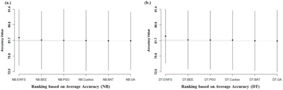
Figure 5.
Scott–Knott ESD statistical rank test representations of the performance (accuracy) of EWFS and metaheuristic search-based WFS methods on NB and DT classifiers. (a) Average accuracy values of NB (b) Average accuracy values of DT.
Figure 6 shows the Scott–Knott ESD statistical rank test results of the proposed EWFS method and the metaheuristics search-based WFS methods we studied on NB and DT based on average AUC values. Significant statistical differences in the average AUC values of NB and DT models based on EWFS methods when compared with metaheuristic search-based WFS were observed. Specifically, NB and DT models based on EWFS outrank and outperform the metaheuristic search-based WFS methods examined. This analysis showed that the high accuracy and low AUC values of models based on metaheuristic search-based WFS might be a result of overfitting, which is one of the inherent problems in metaheuristic search-based WFS, as they can easily get trapped in the local minima. Additionally, similar findings are observed in the case average f-measure value. As indicated in Figure 7, NB and DT models based on the EWFS method outranked and outperformed metaheuristic search-based WFS, as evidenced by a significant statistical difference in the average f-measure values in favor of NB and DT models based on EWFS. Table 6 presents a summary of the Scott–Knott ESD statistical rank test results of NB and DT models based on EWFS and metaheuristic-search-based WFS (GA, PSO, BEE, BAT, and Cuckoo) methods.
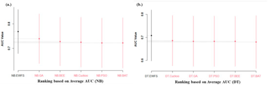
Figure 6.
Scott–Knott ESD statistical rank test representations of the performance (AUC) of EWFS and metaheuristic search-based WFS methods on NB and DT classifiers. (a) Average AUC values of NB (b) Average AUC values of DT.
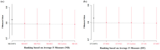
Figure 7.
Scott–Knott ESD statistical rank test representations of the performance (f-measure) of EWFS and metaheuristic search-based WFS methods on NB and DT classifiers. (a) Average F-measure values of NB (b) Average F-measure values of DT.
Table 6.
Analysis of Scott–Knott ESD statistical rank test results of EWFS and metaheuristic search-based WFS methods.
From Table 6, it can be deduced that NB and DT models based on EWFS are superior and rank best when compared against models based on metaheuristic search-based WFS methods. This indicates that there are significant statistical differences in the average performance of models based on EWFS when compared with existing metaheuristic search-based WFS methods, in favor of EWFS methods, based on average accuracy, average AUC, and average f-measure values. This further confirms and supports the superiority of EFWS over existing metaheuristic search-based WFS methods such as GA, PSO, BEE, BAT, and Cuckoo searches for the feature selection process in SDP. However, for generalizability, the performance of EWFS is compared against other forms of WFS which are the sequential search-based WFS in the succeeding subsection.
4.2. Comparison of Proposed EWFS Method against Sequential Search-Based WFS Methods
In this sub-section, the performance of the proposed EWFS is compared with sequential search-based WFS methods. Specifically, the prediction performance of NB and DT models based on the proposed EWFS and WFS are compared using Best First Search (BFS), Greedy Step-wise Search (GDS), Linear Forward Search (LFS), and Sequential Forward Search (SFS).
Figure 8 shows the box-plot representation of average accuracy values of NB and DT models with EWFS and sequential search-based WFS methods. Like the metaheuristic search-based WFS, concerning average accuracy values, the proposed EWFS with NB and DT classifier had superior average accuracy values when compared with NB and DT models based on the sequential search-based WFS method. EWFS with NB and DT recorded an average accuracy value of 82.57% and 83.07%, respectively, compared with metaheuristic search-based WFS methods based on BFS (NB: 81.9%, DT: 81.81%), GDS (NB: 81.93%, DT: 81.88%), LFS (NB: 81.91%, DT: 81.69%), and SFS (NB: 81.88%, DT: 81.8). Specifically, NB and DT models based on EWFS outperformed models based on BFS by +0.8% and +1.54%, GDS by +0.78% and +1.45%, LFS by +0.8% and +1.69%, and SFS by +0.84% and +1.55%, respectively, based on average accuracy values. Based on these analyses, the performance and superiority of EWFS over sequential search-based WFS (BFS, GDS, LFS, and SFS) methods based on average accuracy values can be observed.
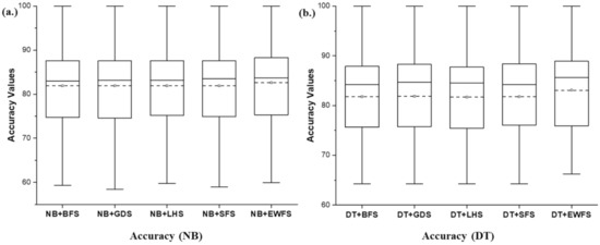
Figure 8.
Box-plot representations of the performance (accuracy) of EWFS and sequential search-based WFS methods on NB and DT classifiers. (a) Average accuracy values of NB (b) Average accuracy values of DT.
Additionally, Figure 9 showcases box-plot representations based on average AUC values of NB and DT models with EWFS and sequential search-based WFS methods. NB and DT classifiers with the EWFS method recorded higher average AUC values when compared against models based on sequential search-based WFS methods. EWFS with NB and DT recorded an average AUC value of 0.768 and 0.708, respectively, compared with metaheuristic search-based WFS methods based on BFS (NB: 0.732, DT: 0.679), GDS (NB: 0.725, DT: 0.668), LFS (NB: 0.731, DT: 0.683), and SFS (NB: 0.733, DT: 0.676). That is, NB and DT models based on EWFS outperformed models based on BFS by +4.92% and +4.66%, GDS by +5.93% and +5.98%, LFS by +5.06% and +3.66%, and SFS by +4.77% and +4.73%, respectively, based on average AUC values.
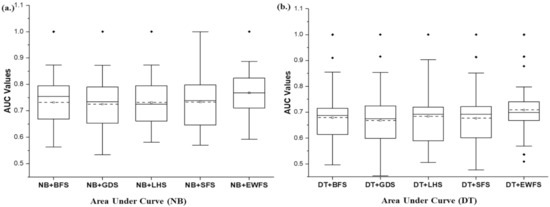
Figure 9.
Box-plot representations of the performance (AUC) of EWFS and sequential search-based WFS methods on NB and DT classifiers. (a) Average AUC values of NB (b) Average AUC values of DT.
Furthermore, Figure 10 presents the box-plot representation based on average f-measure values of NB and DT models with EWFS and sequential search-based WFS methods. Prediction models (NB and DT) with EWFS methods recorded average f-measure values of 0.821 and 0.826, respectively, which are superior to average f-measure values of models based on sequential search-based WFS methods such as BFS (NB: 0.804, DT: 0.808), GDS (NB: 0.801, DT: 0.81), LFS (NB: 0.801, DT: 0.8), and SFS (NB: 0.8, DT: 0.806). Specifically, NB and DT models based on EWFS outperformed models based on LFS by +2.11% and +2.23%, GDS by +2.5% and +1.97%, LFS by +2.5% and +3.25%, and SFS by +2.63% and +2.48%, respectively, based on average f-measure values. Consequently, NB and DT models with EWFS recorded superior f-measure values when compared against models with sequential search-based WFS methods.
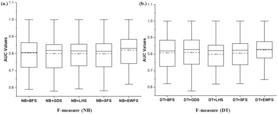
Figure 10.
Box-plot representations of the performance (f-measure) of EWFS and sequential search-based WFS methods on NB and DT classifiers. (a) Average F-measure values of NB (b) Average F-measure values of DT.
In terms of the number of selected features, Table 7 presents and compares the number of selected features by the proposed EWFS and sequential search-based WFS methods. It can be observed that the proposed EWFS selected, on average, a relatively fewer number of features compared with the average number of features selected by the sequential search-based WFS methods studied. In some cases, the sequential search-based WFS (GDS and SFS) selected fewer features than the proposed EWFS. However, EWFS still outperformed these sequential search-based WFS methods (GDS and SFS). Perhaps, the features selected by these methods have low prediction performance, unlike the EWFS, which dynamically selects features based on their relevance while maintaining or enhancing its performance.
Table 7.
Comparison of average selected features by the EWFS and sequential search-based WFS methods.
In addition, as presented in Table 8, the average computational time (in seconds) taken by the proposed EWFS in selecting features is relatively less than the computational time of the sequential search-based WFS methods studied. On NB models, EWFS had a relatively low computational time, although other sequential search-based WFS methods recorded a shorter time. However, in the case of DT models, EWFS had low computational time, which was better than that of the sequential search-based WFS methods, which had high computational times. The high computational time of the sequential search-based WFS methods we tested can be attributed to their respective stagnation and trapping in local optima during the subset evaluation phase. Specifically, EWFS took an average computational time of 3.32 and 4.8 s for selecting an average of five and four features (approximately) for NB and DT models, respectively, as compared with BFS (NB: (4.64 features, 3.24 s), DT: (4.96 features, 21.13 s)), GDS (NB: (2.72 features, 0.7 s), DT: (2.92 features, 2.8 s)), LFS (NB: (4 features, 2.17 s), DT: (4.72 features, 13.76 s)), and SFS (NB: (2.44 features, 1.39 s), DT: (2.96 features, 9.13 s)). The preceding findings demonstrate that the proposed EWFS can select better and more important features in a reasonable computational time. The relatively low computational time for EFWS may be attributed to the re-ranking strategy deployed at the subset evaluation stage for dynamically and iteratively selecting relevant features, thereby reducing the wrapper evaluation cycle, and subsequently computational time.
Table 8.
Comparison of average computational time (in seconds) by the EWFS and sequential search-based WFS methods.
Based on the aforementioned experimental results and findings, it is evident that the proposed EWFS method is superior to existing sequential search-based WFS methods. Nonetheless, further statistical analysis was conducted on the performance of EWFS and the experimented sequential search-based WFS methods using the Scott–Knott ESD statistical rank test to determine the statistically significant differences in their respective performances based on average accuracy, average AUC, and average f-measure values.
Figure 11 shows the Scott–Knott ESD statistical rank test results of the proposed EWFS method and sequential search-based WFS methods on NB and DT based on average accuracy values. As shown in Figure 11, like the metaheuristic search-based WFS case, it can be observed that average accuracy performances of NB and DT based on the EWFS method, although superior, showed no statistically significant differences compared to NB and DT models based on sequential search-based WFS methods. That is, although models based on EWFS had superior average accuracy values, there is not much difference between the average accuracy values of EWFS and existing sequential search-based WFS methods.
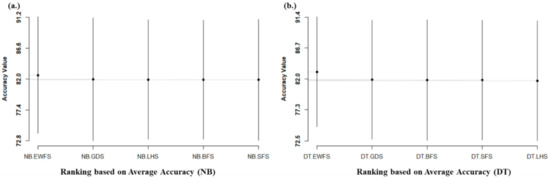
Figure 11.
Scott–Knott ESD statistical rank test representations of the performance (accuracy) of EWFS and sequential search-based WFS methods on NB and DT classifiers. (a) Average accuracy values of NB (b) Average accuracy values of DT.
Figure 12 illustrates the Scott–Knott ESD statistical rank test results of the proposed EWFS method and sequential search-based WFS methods based on average AUC values. There existed significant statistical differences in the average AUC values of NB and DT models based on EWFS methods when compared to sequential search-based WFS. Specifically, NB and DT models based on EWFS outranked and outperformed the sequential search-based WFS methods we tested. These findings suggest that the high accuracy and low AUC values of models based on sequential search-based WFS might be due to overfitting, which is one of the prominent problems in sequential search-based WFS.
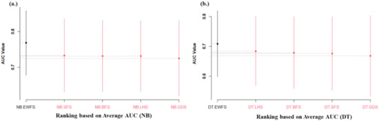
Figure 12.
Scott–Knott ESD statistical rank test representations of the performance (AUC) of EWFS and sequential search-based WFS methods on NB and DT classifiers. (a) Average AUC values of NB (b) Average AUC values of DT.
Furthermore, similar findings were observed in the case of the average f-measure value, as presented in Figure 13. NB and DT models based on the EWFS method outranked and outperformed sequential search-based WFS, as evidenced by significant statistical differences in the average f-measure values in favor of NB and DT models based on EWFS. In summary, Table 9 tabulates the Scott–Knott ESD statistical rank test results of EWFS and sequential search-based WFS (BFS, GDS, LFS, and SFS) methods.
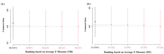
Figure 13.
Scott–Knott ESD statistical rank test representations of the performance (f-measure) of EWFS and sequential search-based WFS methods on NB and DT classifiers. (a) Average F-measure values of NB (b) Average F-measure values of DT.
Table 9.
Analysis of Scott–Knott ESD statistical rank test results of EWFS and sequential search-based WFS methods.
As depicted in Table 9, it can be deduced that NB and DT models based on EWFS are superior and rank best when compared against models based on sequential search-based WFS methods. These findings indicate that there are significant statistical differences in the average performance of NB and DT models based on EWFS when compared with existing sequential search-based WFS methods based on average accuracy, average AUC, and average f-measure values. This further confirms and supports the superiority of the proposed EWFS over existing sequential search-based WFS methods such as BFS, GDS, LFS, and SFS in terms of selecting relevant features at a reasonable computational time in SDP processes.
In summary, the proposed EWFS approach outperformed current metaheuristic and sequential search-based WFS approaches on the analyzed defect datasets in terms of positive effects on the predictive performance of SDP models (NB and DT). These findings, therefore, answer RQ1 and RQ2 (see Section 3.4), as presented in Table 10. As a result, we recommend enhancing the subset evaluation process of WFS methods by deploying a dynamic re-ranking strategy that iteratively selects germane features with a low subset evaluation cycle, while not compromising the prediction performance of the ensuing model.
Table 10.
Answers to research questions.
5. Conclusions and Future Work
This study focuses on resolving the high dimensionality problem in software defect prediction. Specifically, this study addresses the local minima stagnation and computational cost problems of the WFS method by proposing a novel EWFS method. The proposed EWFS method dynamically and iteratively selects optimal features with good prediction performance values for SDP. The proposed EWFS, in particular, was able to produce a more robust and complete subset of features that best represented the datasets we studied. Thus, these results justify the use of a dynamic re-ranking mechanism in the WFS process to improve the subset evaluation time and prediction efficacies of SDP models.
In a broader context, the observations and conclusions of this study can be used by experts and researchers in SDP and other relevant research domains who utilize WFS methods to solve the high dimensionality problem.
As a drawback of this research, there is a need to explore and broaden the application of this research later on by analyzing other WFS system re-ranking configurations with more prediction models. Furthermore, the effects of using ensemble-based WFS as opposed to a single classifier in WFS is worth exploring.
Author Contributions
Conceptualization, A.O.B. (Abdullateef Oluwagbemiga Balogun), S.B., L.F.C. and V.E.A.; Data curation, A.O.B. (Abdullateef Oluwagbemiga Balogun), A.A.I., A.K.A., A.O.B. (Amos Orenyi Bajeh) and G.K.; Formal analysis, A.O.B. (Abdullateef Oluwagbemiga Balogun), A.A.I., M.A.A. and A.K.A.; Funding acquisition, S.M.; Investigation, A.O.B. (Abdullateef Oluwagbemiga Balogun), A.K.A. and G.K.; Methodology, A.O.B. (Abdullateef Oluwagbemiga Balogun) and V.E.A.; Project administration, S.B., L.F.C. and G.K.; Resources, A.O.B. (Abdullateef Oluwagbemiga Balogun), S.M., M.A.A., A.O.B. (Amos Orenyi Bajeh) and G.K.; Software, A.O.B. (Abdullateef Oluwagbemiga Balogun), S.M. and A.O.B. (Amos Orenyi Bajeh); Supervision, S.B., L.F.C., S.M. and A.O.B. (Amos Orenyi Bajeh); Validation, L.F.C., A.A.I., M.A.A. and V.E.A.; Visualization, A.A.I. and M.A.A.; Writing—original draft, A.O.B. (Abdullateef Oluwagbemiga Balogun); Writing—review & editing, Abdullateef Oluwagbemiga Balogun, L.F.C. and V.E.A. All authors have read and agreed to the published version of the manuscript.
Funding
This research was supported by Yayasan Universiti Teknologi PETRONAS (YUTP) Research Grant Scheme under grant numbers (YUTP-FRG/015LC0240) and (YUTP-FRG/015LC0297).
Institutional Review Board Statement
Not applicable.
Informed Consent Statement
Not applicable.
Data Availability Statement
Available on request.
Conflicts of Interest
The authors declare no conflict of interest.
References
- Afzal, W.; Torkar, R. Towards benchmarking feature subset selection methods for software fault prediction. In Computational Intelligence and Quantitative Software Engineering; Springer: New York, NY, USA, 2016; pp. 33–58. [Google Scholar]
- Akintola, A.G.; Balogun, A.; Lafenwa-Balogun, F.B.; Mojeed, H.A. Comparative Analysis of Selected Heterogeneous Classifiers for Software Defects Prediction Using Filter-Based Feature Selection Methods. FUOYE J. Eng. Technol. 2018, 3, 134–137. [Google Scholar] [CrossRef]
- Alazzawi, A.K.; Rais, H.M.; Basri, S.; Alsariera, Y.A.; Capretz, L.F.; Balogun, A.O.; Imam, A.A. HABCSm: A Hamming Based t-way Strategy based on Hybrid. Artificial Bee Colony for Variable Strength Test. Sets Generation. Int. J. Comput. Commun. Control. 2021, 16, 1–18. [Google Scholar] [CrossRef]
- Bajeh, A.O.; Oluwatosin, O.J.; Basri, S.H.U.I.B.; Akintola, A.G.; Balogun, A.O. Object-oriented measures as testability indicators: An empirical study. J. Eng. Sci. Technol. 2020, 15, 1092–1108. [Google Scholar]
- Balogun, A.; Bajeh, A.; Mojeed, H.; Akintola, A. Software defect prediction: A multi-criteria decision-making approach. Niger. J. Technol. Res. 2020, 15, 35–42. [Google Scholar] [CrossRef]
- Ameen, A.O.; Mojeed, H.A.; Bolariwa, A.T.; Balogun, A.O.; Mabayoje, M.A.; Usman-Hamzah, F.E.; Abdulraheem, M. Application of shuffled frog-leaping algorithm for optimal software project scheduling and staffing. In International Conference of Reliable Information and Communication Technology; Springer: New York, NY, USA, 2020. [Google Scholar]
- Balogun, A.O.; Lafenwa-Balogun, F.B.; Mojeed, H.A.; Usman-Hamza, F.E.; Bajeh, A.O.; Adeyemo, V.E.; Adewole, K.S.; Jimoh, R.G. Data sampling-based feature selection framework for software defect prediction. In The International Conference on Emerging Applications and Technologies for Industry 4.0; Springer: Cham, Switzerland, 2020. [Google Scholar]
- Chauhan, A.; Kumar, R. Bug severity classification using semantic feature with convolution neural network. In Computing in Engineering and Technology; Springer: Cham, Switzerland, 2020; pp. 327–335. [Google Scholar]
- Jimoh, R.G.; Balogun, A.O.; Bajeh, A.O.; Ajayi, S. A PROMETHEE based evaluation of software defect predictors. J. Comput. Sci. Its Appl. 2018, 25, 106–119. [Google Scholar]
- Gotlieb, A. Exploiting symmetries to test programs. In Proceedings of the 14th International Symposium on Software Reliability Engineering, Denver, CO, USA, 17–21 November 2003. [Google Scholar]
- Alazzawi, A.K.; Rais, H.M.; Basri, S.; Alsariera, Y.A.; Balogun, A.O.; Imam, A.A. A hybrid artificial bee colony strategy for t-way test set generation with constraints support. J. Phys. Conf. Ser. 2020, 1529, 042068. [Google Scholar] [CrossRef]
- Catal, C.; Diri, B. Investigating the effect of dataset size, metrics sets, and feature selection techniques on software fault prediction problem. Inf. Sci. 2009, 179, 1040–1058. [Google Scholar] [CrossRef]
- Li, L.; Leung, H. Mining static code metrics for a robust prediction of software defect-proneness. In Proceedings of the 2011 International Symposium on Empirical Software Engineering and Measurement, Banff, AB, Canada, 22–23 September 2011. [Google Scholar]
- Mabayoje, M.A.; Balogun, A.O.; Bajeh, A.O.; Musa, B.A. Software defect prediction: Effect of feature selection and ensemble methods. FUW Trends Sci. Technol. J. 2018, 3, 518–522. [Google Scholar]
- Aleem, S.; Capretz, L.F.; Ahmed, F. Comparative performance analysis of machine learning techniques for software bug detection. In Proceedings of the 4th International Conference on Software Engineering and Applications, Vienna, Austria, 19–20 December 2015. [Google Scholar]
- Lessmann, S.; Baesens, B.; Mues, C.; Pietsch, S. Benchmarking Classification Models for Software Defect Prediction: A Proposed Framework and Novel Findings. IEEE Trans. Softw. Eng. 2008, 34, 485–496. [Google Scholar] [CrossRef] [Green Version]
- Li, N.; Shepperd, M.; Guo, Y. A systematic review of unsupervised learning techniques for software defect prediction. Inf. Softw. Technol. 2020, 122, 106287. [Google Scholar] [CrossRef] [Green Version]
- Okutan, A.; Yıldız, O.T. Software defect prediction using Bayesian networks. Empir. Softw. Eng. 2012, 19, 154–181. [Google Scholar] [CrossRef] [Green Version]
- Rodriguez, D.; Herraiz, I.; Harrison, R.; Dolado, J.; Riquelme, J.C. Preliminary comparison of techniques for dealing with imbalance in software defect prediction. In Proceedings of the 18th International Conference on Evaluation and Assessment in Software Engineering, London, UK, 13–14 May 2014. [Google Scholar]
- Usman-Hamza, F.; Atte, A.; Balogun, A.; Mojeed, H.; Bajeh, A.; Adeyemo, V. Impact of feature selection on classification via clustering techniques in software defect prediction. J. Comput. Sci. Appl. 2020, 26, 73–88. [Google Scholar] [CrossRef]
- Balogun, A.; Oladele, R.; Mojeed, H.; Amin-Balogun, B.; Adeyemo, V.E.; Aro, T.O. Performance analysis of selected clustering techniques for software defects prediction. Afr. J. Comput. ICT 2019, 12, 30–42. [Google Scholar]
- Rodriguez, D.; Ruiz, R.; Cuadrado-Gallego, J.; Aguilar-Ruiz, J.; Garre, M. Attribute selection in software engineering datasets for detecting fault modules. In Proceedings of the 33rd EUROMICRO Conference on Software Engineering and Advanced Applications (EUROMICRO 2007), Lubeck, Germany, 28–31 August 2007. [Google Scholar]
- Wang, H.; Khoshgoftaar, T.M.; van Hulse, J.; Gao, K. Metric selection for software defect prediction. Int. J. Softw. Eng. Knowl. Eng. 2011, 21, 237–257. [Google Scholar] [CrossRef]
- Rathore, S.S.; Gupta, A. A comparative study of feature-ranking and feature-subset selection techniques for improved fault prediction. In Proceedings of the 7th India Software Engineering Conference, Chennai, India, 19–21 February 2014. [Google Scholar]
- Xu, Z.; Liu, J.; Yang, Z.; An, G.; Jia, X. The impact of feature selection on defect prediction performance: An empirical comparison. In Proceedings of the IEEE 27th International Symposium on Software Reliability Engineering (ISSRE), Ottawa, ON, Canada, 23–27 October 2016. [Google Scholar]
- Balogun, A.O.; Basri, S.; Jadid, S.A.; Mahamad, S.; Al-momani, M.A.; Bajeh, A.O.; Alazzawi, A.K. Search-based wrapper feature selection methods in software defect prediction: An empirical analysis. In Computer Science On-line Conference; Springer: Cham, Switzerland, 2020. [Google Scholar]
- Ghotra, B.; McIntosh, S.; Hassan, A.E. A large-scale study of the impact of feature selection techniques on defect classification models. In Proceedings of the IEEE/ACM 14th International Conference on Mining Software Repositories (MSR), Buenos Aires, Argentina, 20–28 May 2017. [Google Scholar]
- Balogun, A.O.; Basri, S.; Mahamad, S.; Abdulkadir, S.J.; Almomani, M.A.; Adeyemo, V.E.; Al-Tashi, Q.; Mojeed, H.A.; Imam, A.A.; Bajeh, A.O. Impact of Feature Selection Methods on the Predictive Performance of Software Defect Prediction Models: An Extensive Empirical Study. Symmetry 2020, 12, 1147. [Google Scholar] [CrossRef]
- Balogun, A.O.; Basri, S.; Capretz, L.F.; Mahamad, S.; Imam, A.A.; Almomani, M.A.; Adeyemo, V.E.; Kumar, G. An adaptive rank aggregation-based ensemble multi-filter feature selection method in software defect prediction. Entropy 2021, 23, 1274. [Google Scholar] [CrossRef]
- Balogun, A.O.; Basri, S.; Abdulkadir, S.J.; Hashim, A.S. Performance Analysis of Feature Selection Methods in Software Defect Prediction: A Search Method Approach. Appl. Sci. 2019, 9, 2764. [Google Scholar] [CrossRef] [Green Version]
- Anbu, M.; Mala, G.S.A. Feature selection using firefly algorithm in software defect prediction. Clust. Comput. 2017, 22, 10925–10934. [Google Scholar] [CrossRef]
- Kakkar, M.; Jain, S. Feature selection in software defect prediction: A comparative study. In Proceedings of the 6th International Conference on Cloud System and Big Data Engineering, Noida, India, 14–15 January 2016. [Google Scholar]
- Al-Tashi, Q.; Kadir, S.J.A.; Rais, H.M.; Mirjalili, S.; Alhussian, H. Binary Optimization Using Hybrid Grey Wolf Optimization for Feature Selection. IEEE Access 2019, 7, 39496–39508. [Google Scholar] [CrossRef]
- Al-Tashi, Q.; Rais, H.; Jadid, S. Feature selection method based on grey wolf optimization for coronary artery disease classification. In Proceedings of the 3rd International Conference of Reliable Information and Communication Technology (IRICT), Kuala Lumpur, Malaysia, 23–24 July 2018. [Google Scholar]
- Balogun, A.O.; Basri, S.; Abdulkadir, S.J.; Sobri, A.H. A hybrid multi-filter wrapper feature selection method for software defect predictors. Int. J. Supply Chain. Manag. 2019, 8, 916–922. [Google Scholar]
- Gao, K.; Khoshgoftaar, T.M.; Wang, H.; Seliya, N. Choosing software metrics for defect prediction: An investigation on feature selection techniques. Software Pr. Exp. 2011, 41, 579–606. [Google Scholar] [CrossRef] [Green Version]
- Wahono, R.S.; Suryana, N.; Ahmad, S. Metaheuristic optimization based feature selection for software defect prediction. J. Softw. 2014, 9, 1324–1333. [Google Scholar] [CrossRef] [Green Version]
- Song, Q.; Jia, Z.; Shepperd, M.; Ying, S.; Liu, J. A General Software Defect-Proneness Prediction Framework. IEEE Trans. Softw. Eng. 2010, 37, 356–370. [Google Scholar] [CrossRef] [Green Version]
- Muthukumaran, K.; Rallapalli, A.; Murthy, N.B. Impact of feature selection techniques on bug prediction models. In Proceedings of the 8th India Software Engineering Conference, Bangalore, India, 18–20 February 2015. [Google Scholar]
- Rodríguez, D.; Ruiz, R.; Cuadrado-Gallego, J.; Aguilar-Ruiz, J. Detecting fault modules applying feature selection to classifiers. In Proceedings of the IEEE International Conference on Information Reuse and Integration, Las Vegas, NV, USA, 13–15 August 2007. [Google Scholar]
- Cynthia, S.T.; Rasul, M.G.; Ripon, S. Effect of feature selection in software fault detection. In International Conference on Multi-disciplinary Trends in Artificial Intelligence; Springer: Cham, Switzerland, 2019. [Google Scholar]
- Ekundayo, A. Wrapper feature selection based heterogeneous classifiers for software defect prediction. Adeleke Univ. J. Eng. Technol. 2019, 2, 1–11. [Google Scholar]
- Ding, Z. Isolation forest wrapper approach for feature selection in software defect prediction. In IOP Conference Series: Materials Science and Engineering; IOP Publishing: Bristol, UK, 2021. [Google Scholar]
- Yu, Q.; Jiang, S.; Zhang, Y. The performance stability of defect prediction models with class imbalance: An empirical study. IEICE Trans. Inf. Syst. 2017, 100, 265–272. [Google Scholar] [CrossRef] [Green Version]
- Bermejo, P.; Gámez, J.A.; Puerta, J.M. Adapting the CMIM algorithm for multilabel feature selection. A comparison with existing methods. Expert Syst. 2017, 35, e12230. [Google Scholar] [CrossRef]
- Yang, X.-S.; Deb, S. Multiobjective cuckoo search for design optimization. Comput. Oper. Res. 2013, 40, 1616–1624. [Google Scholar] [CrossRef]
- Shepperd, M.; Song, Q.; Sun, Z.; Mair, C. Data Quality: Some Comments on the NASA Software Defect Datasets. IEEE Trans. Softw. Eng. 2013, 39, 1208–1215. [Google Scholar] [CrossRef] [Green Version]
- Kondo, M.; Bezemer, C.-P.; Kamei, Y.; Hassan, A.E.; Mizuno, O. The impact of feature reduction techniques on defect prediction models. Empir. Softw. Eng. 2019, 24, 1925–1963. [Google Scholar] [CrossRef]
- Wu, R.; Zhang, H.; Kim, S.; Cheung, S.C. Relink: Recovering links between bugs and changes. In Proceedings of the 19th ACM SIGSOFT Symposium and the 13th European Conference on Foundations of Software Engineering, Szeged, Hungary, 5–9 September 2011. [Google Scholar]
- Song, Q.; Guo, Y.; Shepperd, M. A Comprehensive Investigation of the Role of Imbalanced Learning for Software Defect Prediction. IEEE Trans. Softw. Eng. 2018, 45, 1253–1269. [Google Scholar] [CrossRef] [Green Version]
- Nam, J.; Fu, W.; Kim, S.; Menzies, T.; Tan, L. Heterogeneous defect prediction. IEEE Trans. Softw. Eng. 2017, 44, 874–896. [Google Scholar] [CrossRef] [Green Version]
- Tantithamthavorn, C.; McIntosh, S.; Hassan, A.E.; Matsumoto, K. The Impact of Automated Parameter Optimization on Defect Prediction Models. IEEE Trans. Softw. Eng. 2018, 45, 683–711. [Google Scholar] [CrossRef] [Green Version]
- Balogun, A.O.; Basri, S.; Abdulkadir, S.J.; Mahamad, S.; Al-momamni, M.A.; Imam, A.A.; Kumar, G.M. Rank aggregation based multi-filter feature selection method for software defect prediction. In Proceedings of the International Conference on Advances in Cyber Security, Penang, Malaysia, 30 July–1 August 2020. [Google Scholar]
- Balogun, A.O.; Basri, S.; Mahamad, S.; Abdulkadir, S.J.; Capretz, L.F.; Imam, A.A.; Almomani, M.A.; Adeyemo, V.E.; Kumar, G. Empirical analysis of rank aggregation-based multi-filter feature selection methods in software defect prediction. Electronics 2021, 10, 179. [Google Scholar] [CrossRef]
- James, G.; Witten, D.; Hastie, T.; Tibshirani, R. An Introduction to Statistical Learning; Springer: New York, NY, USA, 2013; Volume 112. [Google Scholar]
- Kuhn, M.; Johnson, K. Applied Predictive Modeling; Springer: Berlin, Germany, 2013; Volume 26. [Google Scholar]
- Balogun, A.O.; Adewole, K.S.; Raheem, M.O.; Akande, O.N.; Usman-Hamza, F.E.; Mabayoje, M.A.; Akintola, A.G.; Asaju-Gbolagade, A.W.; Jimoh, M.K.; Jimoh, R.G.; et al. Improving the phishing website detection using empirical analysis of Function Tree and its variants. Heliyon 2021, 7, e07437. [Google Scholar] [CrossRef]
- Hall, M.; Frank, E.; Holmes, G.; Pfahringer, B.; Reutemann, P.; Witten, I.H. The WEKA data mining software: An update. ACM SIGKDD Explor. Newsl. 2009, 11, 10–18. [Google Scholar] [CrossRef]
- Crawley, M.J. The R Book; John Wiley & Sons: Hoboken, NJ, USA, 2012. [Google Scholar]
Publisher’s Note: MDPI stays neutral with regard to jurisdictional claims in published maps and institutional affiliations. |
© 2021 by the authors. Licensee MDPI, Basel, Switzerland. This article is an open access article distributed under the terms and conditions of the Creative Commons Attribution (CC BY) license (https://creativecommons.org/licenses/by/4.0/).