
Space, Matter and Interactions in a Quantum Early Universe Part I: Kac–Moody and Borcherds Algebras


1
Istituto Nazionale Fisica Nucleare (INFN) , Sez. di Genova, Via Dodecaneso 33, I-16146 Genova, Italy
2
Quantum Gravity Research (QGR), 101 S. Topanga Canyon Rd., 1159, Los Angeles, CA 90290, USA
3
Centro Studi e Ricerche Enrico Fermi, Via Panisperna 89A, I-00184 Roma, Italy
*
Author to whom correspondence should be addressed.
Symmetry 2021, 13(12), 2342; https://doi.org/10.3390/sym13122342
Submission received: 29 October 2021
/
Revised: 29 November 2021
/
Accepted: 1 December 2021
/
Published: 6 December 2021
(This article belongs to the Special Issue Modified Gravity, Supergravity and Cosmological Applications)
Abstract
:We introduce a quantum model for the universe at its early stages, formulating a mechanism for the expansion of space and matter from a quantum initial condition, with particle interactions and creation driven by algebraic extensions of the Kac–Moody Lie algebra . We investigate Kac–Moody and Borcherds algebras, and we propose a generalization that meets further requirements that we regard as fundamental in quantum gravity.
1. Introduction
This is the first of two papers—see also [1]—describing an algebraic model of quantum gravity.
The intrinsic difficulty of quantizing gravity, encountered also in the most acclaimed approaches of string theory and loop quantum gravity, has led us to this attempt of thinking outside the box and exploiting only the most fundamental principles of quantum mechanics and general relativity, as we believe that they should apply in the extreme conditions of a hot dense universe in its early stages. We use, therefore, an Occam’s razor type of approach by starting with the least possible assumptions and filling in more structure when needed.
Two fundamental and intuitive physical principles are assumed to hold in the regime we study:
- FP1
- There is no classical observable to bequantized. We start directly from quantum objects and states of the system: interactions, creation and the expansion of spacetime all occur with quantum probability amplitudes; the universe evolves from an initial quantum state. Gravity is identified with the way spacetime is created as particles evolve, whereas the rest of the dynamics, which incorporate electro-weak and strong forces, only depend on the quantum charges of the constituents and the rule for the building blocks of the interactions, which we assume to be algebraic in nature. We depart from the conventional view that quantum gravity should be realized as the quantization of gravity with its renormalization, with the four fundamental forces unifying at the Planck scale. We are at the Plank scale: the charges of the constituents are symmetrical, but diversity comes from quantum theory itself, and from the initial conditions.
- FP2
- There is no spacetime geometry to start with. We can only start by establishing one rule for the interactions and one for the creations of spacetime, bearing in mind that they both occur with probability amplitudes: both interactions and spacetime have an intrinsic quantum nature.The assumption, supported by physical observations, that at very high temperatures the interactions are tree-like, has led us to consider algebraic models, with the algebra product playing the role of the building blocks of all interactions. A mechanism for the quantum creation of spacetime suggests the inclusion of momenta within the charges (roots) of the algebra, thus achieving both charge and energy–momentum conservation. We reach this goal by considering infinite dimensional generalized Lie algebras. A generator in the algebra is related to a particle, with certain charges coming from the algebra roots, but it is also related to a quantum field, since new generators are produced by multiplication in the algebra: a generator expands in spacetime with complex quantum amplitudes, but locally interacts, disappears and contributes to the creation of new generators. This local action can be considered as a vertex, made of generators obeying the rules of an algebra. There is no vacuum, since space points exist only where generators are. We see, therefore, that we do have an algebra at the core of the model, but the expansion of spacetime embeds it into a larger picture: that of a vertex-type algebra describing quantum interactions and a quantum-generated spacetime.
We believe that the above considerations are plausible and strongly based on fundamental physics. The evolution of the universe, its quantum interactions and quantum expansion from a chosen initial state of a finite set of generators, can be turned into an algorithm in which all physical quantities are, in principle, calculable, and no infinity occurs. A concrete, calculable realization of the above ideas is what we have achieved with our model, which has no claim other than being physically consistent and mathematically rigorous.
In this first paper, we provide an introduction to the foundations of the model, and we start investigating the mathematical structures that suit our purpose. In the second paper [1], we will deal with a physical model relying on a particular infinite dimensional algebra.
The Lie algebra at the core of our model has the following features and interpretation:
- (1)
- It is an infinite dimensional Lie algebra extending that is regarded as the internal quantum number subalgebra, meaning that the roots represent the charges and spin of elementary particles;
- (2)
- Its root lattice is Lorentzian;
- (3)
- The subspace of the lattice that is complementary to that of is interpreted as momentum space.
Remark 1.
The Lie algebra has been considered by many as a possible algebra for grand unification, as well as for quantum gravity. It has then been considered not suitable after the no-go theorem by Distler and Garibaldi [2]. We will show in Section 2.3 how fulfils the requirements for standard model degrees of freedom and algebras, which seems to contradict the thesis of Distler and Garibaldi. We underline here that it does not, since the hypothesis, denoted TOE1 by the authors of [2]—in particular, the fact that the algebra of the standard model centralizes —not only does not apply, but actually needs not to do so, as will become obvious in the development of Section 2.3.
Algebraic methods are extensively used and successfully exploited in string theory and conformal field theory in two dimensions, through the concept of vertex operator algebras, [3,4,5], in order to describe the interactions between different strings, localized at vertices, analogously to the Feynman diagram vertices. Mathematically, the underlying concept of a vertex algebra was introduced by Borcherds [6,7,8], in order to prove the Monstrous Moonshine conjecture [9].
Infinite dimensional Kac–Moody algebras have recently entered the loop quantum gravity literature to describe spin network edge modes (generalizing the Gibbons–Hawking boundary term); e.g., [10,11], in which a boundary symmetry was found, along with a Virasoro structure that resembles strings with an internal three-dimensional structure. On the other hand, the Kac–Moody algebra e has been investigated in string theory and M-theory by P. West and collaborators (cf. e.g., [12] and Refs. therein). As we will elucidate further below, we consider a Borcherds extension of the even larger Kac–Moody algebra e in order to describe all interactions in a very early universe, and texploit the Grassmann envelop in order to deal with fermions and implement Pauli’s exclusion principle.
The algebras used in this paper may be regarded as vertex operator algebras in a broader sense, since they are characterized by interaction operators that look like generators of a Lie algebra, and whose product depends upon parameters related to the spacetime creation and expansion. The Lie algebra acts locally, but it is immersed in a wider, vertex-type algebra by means of a mechanism that creates a discrete quantum spacetime.
The Pauli exclusion principle is fulfilled by turning the algebra into a Lie superalgebra using the Grassmann envelope.
The resulting model is thus intrinsically relativistic, both because of the way spacetime expands and because the Poincaré group acts locally on the Lie algebra. Furthermore, the conservation of charge and momentum is a consequence of the Lie product, and, in this respect, they are treated at the same level.
1.1. , a Lie Algebra for Quantum Gravity
At a very fundamental level, we make the following assumptions on quantum gravity, founded on the current theoretical and experimental knowledge in physics.
- (QG.1)
- Gravity is a characteristic of spacetime;
- (QG.2)
- Spacetime is dynamical and related to matter. Therefore, we assume that it emerges from the existence of particles and their interactions. There is no way of defining distances and time lapses without interactions, so that the creation and expansion of spacetime is itself a rule followed by particle interactions;
- (QG.3)
- A suitable mathematical structure at the core of the description of quantum gravity is that of an algebra, which we will henceforth denote by , whose generators represent the particles and whose product yields the building blocks of the interactions (let us call them elementary interactions). As a consequence, the interactions are endowed with a tree structure, thus opening up the opportunity for a description of scattering amplitudes in terms of what we would call gravitahedra, providing a generalization of the associahedra and permutahedra in the current theory of scattering [13,14,15,16,17,18,19,20]. The structure constants of the algebra determine the quantum amplitudes of the elementary interactions; in particular, we assume to be a Lie algebra because it enables us to derive the fundamental conservation laws observed in physics directly from the action of the generators as derivations (Jacobi identity). As in the theory of fields, the interactions may only occur locally, point-by-point in the expanding spacetime, which can therefore be viewed as a parameter on which the algebra product depends;
- (QG.4)
- In agreement with the theory of a big bang, strongly supported by the current observations, we assume the existence of an initial quantum state, mathematically represented by an element of the universal enveloping algebra of . Such an element is made of generators that can all interact among themselves, thus yielding the first geometrical interpretation: that of a point where particles may interact;
- (QG.5)
- A particle has a certain probability amplitude to interact but also not to interact, in which case, it expands, as described in Section 1.2;
- (QG.6)
- Particles are quantum objects, hence their existence through interactions occurs with certain amplitudes. Therefore, spacetime acquires a quantum structure: a point in space and time where particles are present with a certain amplitude and may interact. The amplitude related to the quantum spacetime point is the sum of the amplitudes for particles to be there. Consequently, the fact that gravitation appears as an attractive force has to be explained through amplitudes and their interference;
- (QG.7)
- The initial set of generators is finite by assumption, being the the initial state represented by an element of the universal enveloping algebra. These generators are all allowed to interact with each other with a certain amplitude and according to the algebra relations, at what we call time 0 of the universal clock. The outcome of the first finite number of interactions, plus the creation of space, which is a consequence of the momentum part of the root associated with each generator, leads to a second finite set of interactions, and so on. What we call universal time is this order parameter of the interactions. The expansions are also countable, hence discrete: the structure of spacetime that emerges is discrete and finite at every instant of the universal clock, as is the universe and the quantum theory describing it. There is no divergence of any sort: quantum field theory in the continuum, with its divergences and related renormalizations, is an approximation that may be useful for calculations long after the big bang;
- (QG.8)
- The finiteness of the expanding universe, and thus the absence of spacetime beyond it, affects the quantum initial state of particles, which are not free to move on the spacetime stage but are bound as if they were surrounded by infinitely high barriers. The steady state of such a particle is a superposition of states with opposite 3-momenta, representing an object that moves simultaneously in opposite directions, where, by 3-momentum, we denote the spatial component of 4-momentum.
1.2. Expansion
The assignment of opposite 3-momenta is inherent to the quantum behavior of a particle in a box, in which, the square of the momentum, but not the momentum itself, has a definite value in a stationary state. In standard relativistic and non-relativistic quantum mechanics, the ground state is a superposition of generalized states, with opposite momenta and . We maintain the same energy and start enlarging the box on opposite sides along the direction of in steps of in Planck units, so that a massless particle travels at velocity c, and a massive one travels slower than that. We obtain a wave proportional to for and .
The wave function for the first four expansions is shown in Figure 1. We take the discretized picture of the sine function maxima and minima, the dots, with cosmological time .
The amplitude also acquires a time-dependent phase that makes it complex.
1.3. Fermions and Bosons
The Lie algebras considered in this paper contain , and thus . Under the adjoint action of , the generators of split into spinorial and non-spinorial ones, providing the algebra with a two-graded structure. We give the spinorial generators the physical meaning of fermions, whereas the non-spinorial generators are given the physical meaning of bosons, in order to automatically comply with the addition of angular momenta.
On the other hand, the Pauli exclusion principle is embodied in the Grassmann envelope, which turns the two-graded algebra into a Lie superalgebra. The degrees of freedom of the spin-1/2 fermions originate from the superposition of opposite 3-momenta and the corresponding change in helicity caused by the reflection at the space boundary. The Poincaré group then naturally emerges as a group of transformations of the local algebra , leaving the charges invariant.
All of these topics will be treated in the companion paper [1].
1.4. Quantum Quasicrystal
The expansion of the space that we propose has two fundamental features:
- A space point may exist with a certain probability amplitude, this latter being the sum of the amplitudes for some particles—matter or radiation—to be there: no space point can possibly be empty;
- Space is a quantum object that expands according to algebraic rules.
2. , the Charge/Spin Subalgebra
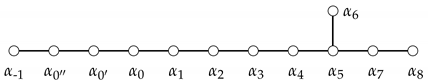
In our treatment, we use the following labels for the Dynkin diagram of :
![Symmetry 13 02342 i001]()

A way of writing the simple roots of in the orthonormal basis of is:
The whole root system of (obtained from the simple roots by Weyl reflections) can be written as follows:
The first set of 112 roots is the set of roots of . The set is a Weyl spinor of , with respect to the adjoint action (every orthogonal Lie algebra in even dimension has a Weyl spinor representation of dimension ).
If is a root, there is a unique way of writing it as , where the ’s are simple (in fact, all ’s are positive for positive roots, and negative for negative roots). The sum is called the height of .
The fact that the roots of are the roots of a subalgebra and those of correspond to a representation of it can be seen by noticing that: , . Moreover, implies that is embedded into in a symmetric way.
Thus, one can consistently define a non-Cartan generators bosonic if , and fermionic if . We also call fermionic or bosonic the root associated to a fermionic (resp. bosonic) non-Cartan generator . A Cartan generator is always bosonic for any , since . The roots of split into 128 fermions (F) and 112 bosons (B).
2.1. Algebraic Structure
The algebra can be defined from its root system [24,25,26], over the complex field extension of the rational integers in the following way:
- (a)
- We select the set of simple roots of ;
- (b)
- We select a basis of the eight-dimensional vector space over and set for each , such that ;
- (c)
- We associate to each a one-dimensional vector space over spanned by ;
- (d)
- We define as a vector space over ;
- (e)
Definition 1.
Let denote the lattice of all linear combinations of the simple roots with integer coefficients
the asymmetry function is defined by:
where and
Proposition 1.
For each , the scalar product ; (respectively, ) is a root if and only if (respectively, ); if both and are not in , then .
For if is a root, then is not a root.
The following properties of the asymmetry function follow from its definition [26].
Proposition 2.
The asymmetry function ε satisfies, for :
Property shows that the product in (4) is indeed antisymmetric.
2.2. Charges and the Magic Star
There are four orthogonal ’s in , where orthogonal means that the planes on which their root systems lie are orthogonal to each other.
We denote one of them for color, one for flavor and the other two as and :
: ,
: ,
The generators of and are bosonic.
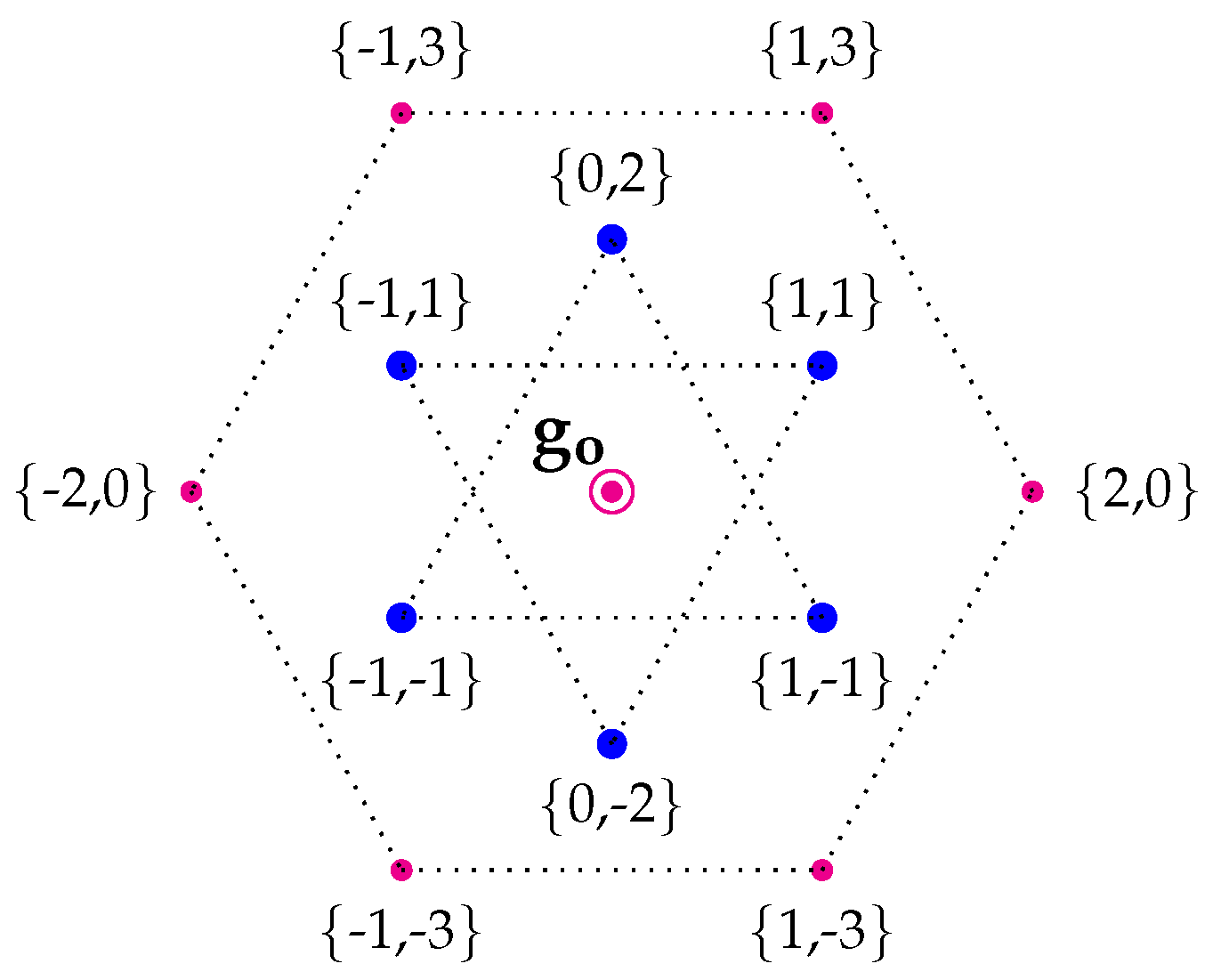
The Magic Star (MS) of shown in Figure 2 is obtained by projecting its roots on the plane of [28]. The pair of integers are the (Euclidean) scalar products and for each root . The fermions on the tips of the MS are quarks, since they are acted upon by : they are colored. The fermions within the center of the MS are leptons: they are colorless. A similar MS of within is obtained by projecting the roots in the center of the MS of on the plane of .
Notice that, in each tip of the MS of , we obtain 27 roots, 11 of which are bosonic and 16 fermionic; this corresponds to the following decomposition of the irrepr. of
On the other hand, within , we have nine roots in each tip of the MS, five of which are bosonic and four fermionic; this corresponds to the following decomposition of the repr. of :
Table A1, Table A2, Table A3 and Table A4 in Appendix A describe the content of these MS, root by root.
The magic of the MS is that each tip of the star, , both in the case of and of , can be viewed as a cubic (simple) Jordan algebra , over the octonions and the complex field, respectively, and each pair of opposite tips, with respect to the center of the star, has a natural algebraic structure of a Jordan pair. The algebra in the center of the star is the derivation algebra of the Jordan pair; when the Jordan pair is made of a pair of Jordan algebras, its derivations also define the Lie algebra of the structure group of the Jordan algebra itself [28,29,30,31].
2.3. The Standard Model
In this section, we relate the charges to the degrees of freedom of the Standard Model (SM) of elementary particle physics. It is not our aim to carry through a detailed analysis; in particular, we do not consider symmetry breaking, nor the Higgs mechanism, nor chirality and parity violation by weak interactions in the fermionic sector. We do, however, focus on spin as an internal degree of freedom, and this will be instrumental for the treatment of the Poincaré action on our algebra, which we will investigate in the companion paper [1].
The first important step, after splitting the roots into colored and colorless, as in the previous section, is to find the electromagnetic that gives the right charges to quarks and leptons. The choice may not be unique, although is strongly limited by the requirement to yield the right charges, but the one we make is certainly consistent. We select the generated by
giving to , where , the charge
where
The second column of Table A1, Table A2, Table A3 and Table A4 in Appendix A shows the charges of the generators , with shown in the first column. In particular, Table A3 and Table A4 show the charges given to quarks and leptons.
We now select the semi-simple Lie algebra with roots (other choices would be equivalent; thus, this does not imply any loss of generality). We denote by the roots and , respectively, by , the subalgebra of associated to the roots , and by , the one associated to the roots . The non-Cartan generators of fall into irreducible representations of spin :
where corresponds to the six components as a rank 2 antisymmetric tensor in four dimensions, with selfdual and antiselfdual parts and , respectively. Notice that all fermions have a half-integer spin or , whereas all bosons of type have an integer spin.
In order to define the action of the Poincaré group in [1], we need the covering group of rotations in the internal space. For this purpose, we select the spin (diagonal) subalgebra as the compact (real) form with generators
The representation splits into a scalar and a vector under this rotation subalgebra. The spin-1 particle within is the linear span of the generators with z-component of spin and with ; the corresponding scalar is , as it can be easily verified.
2.3.1.
Let us now consider the bosons. There are not many choices for them; indeed, they must be colorless vectors with respect to and have electric charge . The bosons are therefore the generators associated to (within mentioned in Section 2.2) and , and the electric charge given by the presence of ; they change flavor to both quarks and leptons. The above analysis suggests that the extra degree of freedom needed, say, for , to become massive, from the two degrees of freedom of the massless helicity-1 state, is , as a part of the Higgs mechanism, which we will not discuss any further in this paper.
Remark 2.
We could have made other equivalent choices for the subalgebra, which has to act non-trivially on : once passing to real forms, it cannot possibly commute with the weak interaction . For what concerns the no-go theorem by Distler–Garibaldi, the hypothesis TOE1 of [2] cannot possibly apply, as outlined in the introduction; see Remark 1. We also emphasize that, contrary to [2], we are dealing with the complex form of because we want complex phases for the particle states.
Using the properties of the asymmetry function and the ordering of the simple roots , we obtain:
hence, the massive is described by three components:
Moreover, using the notation
we obtain
and
These commutation relations correspond to the action of the rotation matrices:
regarding the vectors, in the spherical basis , which corresponds, for angular momentum 1, to the spherical harmonic basis for the irreducible representations of . With respect to the same vector in the standard orthogonal basis , we have:
The transformation between (column) vectors in the two bases is represented by the unitary matrix U:
The correspondence with R’s and W’s is:
Remark 3.
We have an interesting relationship between the weak and rotation generators in the internal space (spin generators) by noticing that
and, consequently, the relation with .
2.3.2.
We associate the boson with spin , denoted by , to the vector orthogonal to in the plane of and ; hence, it is, up to a scalar, the Cartan generator . It interacts with left-handed neutrinos and right-handed antineutrinos, contrary to the photon; it does not allow for flavor-changing neutral currents.
Notice that the generator of hypercharge of the standard model is, in this, the setting compact Cartan generator , where . The Weinberg angle is the angle between the axis representing the photon and the axis representing the hypercharge; therefore, , where is the angle between and , and we obtain .
Since , ; hence, we have the following commutation relations:
that is
We want , as a spin-1 particle, to obey the same commutation relations with the rotation generators as . We can define the spin components of this way by a comparison with the last commutator in each row of (18):
(see (14) for the definition of ).
By looking at Table A3 in Appendix A, we notice that interacts, for instance, with with spin to give with spin , and, similarly, for other leptons and for quarks. In particular, there are no flavor-changing neutral currents.
2.3.3. The Tables at a Glance
From the Table A1, Table A2, Table A3 and Table A4 in Appendix A, one can deduce all the standard model charges (in particular, we have denoted with a prime possible mixings in Table A3 and Table A4). We have:
- (SM.1)
- The color charges are denoted by the pair , and one can associate colors to them—say, , and —and, similarly, for the anti-colors;
- (SM.2)
- The quarks are the fermions in Table A1 with a certain color; they come in three color families, and anti-quarks have anti-colors and opposite electric charges with respect to quarks;
- (SM.3)
- The gluons are the generators of , change color to the quarks on which they act, as on a or representation, and their electric charge is 0;
- (SM.4)
- (SM.5)
- The leptons have an integer electric charge in ;
- (SM.6)
- There are four flavor families; we have used the notation for the fourth lepton family and for the fourth quark family;
- (SM.7)
The consequences of this classification, with respect to the Poincaré action on , will be discussed in the companion paper [1].
3. The Kac–Moody Algebras
Let denote the Kac–Moody algebra associated to the Cartan matrix A, with Cartan subalgebra . For all algebras in this paper, A is symmetric; its entries are denoted by . We denote the Chevalley generators by , associated to the simple root , and by , associated to the root . Let (resp. ) denote the subalgebra of generated by (resp.). By Theorem 1.2 (a), (e) in [27], the following triangular decomposition holds:
Note that, for a root (resp. ), we have , the dual of , and the vector space is the linear span of the elements of the form (resp. ), such that (resp. ). The multiplicity of a root is defined as ( for each simple root ).
Kac–Moody algebras [27,32] can be tackled in terms of simple roots and their (extended) Dynkin diagram, or, equivalently, their Cartan matrix, without any reference to root coordinates. Some physical features or interpretations may, however, be more explicit when roots are expressed on an orthonormal basis rather than on a simple root basis. This is the case of this paper, in which some root coordinates, except for the case of , are interpreted as momentum coordinates. We recall that the metric is Euclidean for , but Lorentzian in the case of .
Our notation for the simple roots is shown in the Dynkin diagram of :
![Symmetry 13 02342 i002]() Analogous diagrams are those of (without ), of (without ) and of (without ).
Analogous diagrams are those of (without ), of (without ) and of (without ).
3.1. The Simple Roots of and
We introduce the following set of simple roots of in terms of the basis vectors spanning the Lorentzian space , with and , for :
All of these roots have norm 2, with respect to the scalar product , and the corresponding Cartan matrix is the Gram matrix of the even unimodular Lorentzian lattice made of all the vectors in , whose components are all in or all in and have an integer scalar product with , as can be easily checked.
The affine Kac–Moody algebra is obtained by eliminating the root . Notice that
where is the lowest height root of and is a light-like vector.
3.2.
The Cartan subalgebra of is the span of 10 generators, containing two new ones with respect to . We write
where
and K is a central element.
Let be the root system of , be its Cartan subalgebra, (resp. ) be a Cartan (resp. non-Cartan) generator associated to the root , for be a Cartan generator associated to the simple root and X and Y be either Cartan or non-Cartan generators of . It is shown by Kac [27] that:
- The root system of is
- is determined by the following commutation relations:where is Kac’s asymmetry function, see Section 2.1;
- The commutation relations in are the same as those for the central extended loop algebra of plus derivations:with the following correspondenceand with the invariant non-degenerate symmetric bilinear form defined by:
For (roots of ) and the letter h referring to a Cartan generator, the commutation relations, with no reference to the loop algebra, are:
Remark 4.
The commutation relations of are essentially determined by those of , whose main ingredient for explicit calculations is the asymmetry function.
Remark 5.
The second correspondence in (37) shows why the so called imaginary roots are eight-fold degenerate: the space of generators associated to each root is indeed an eight-dimensional space isomorphic to the span of , namely the Cartan subalgebra of .
3.3. in a Dimensional Toy Model
The explicit construction presented here, using a realization of the roots in terms of the orthonormal basis of , suggests letting the coordinates relate to charge/spin degrees of freedom, and interpreting the coordinates as 2-momentum coordinates with a Lorentzian signature.
A crucial step in our model, which describes a universe that expands from an initial quantum state, is to restrict the particles forming that state, and hence their interactions, to lie in the subalgebra of the triangular decomposition Equation (28) of (the reason will be explained in item (TM.3) below). The restriction to has the following consequences:
- (TM.1)
- We remark that in the last commutation relation implies that either or is negative, hence , being and, in particular, in whenever is a negative root of ;
- (TM.2)
- The roots involved in the interactions are not only real; for instance, are positive roots and . Therefore, by Proposition 5.1 of [27], at least and are roots; the outgoing generator of the interaction between and is similar to the Cartan generator , except that it carries a momentum . This yields the interesting consideration that neutral radiation fields, like the photon, are not associated to Cartan elements of infinite dimensional Kac–Moody algebras, but to imaginary roots, a feature that is not present in Yang–Mills theories. It is also worth noticing that the second equation in (41) implies that the neutral radiation field keeps memory of the particle–antiparticle pair that produced it, represented in the equation by the root ;
- (TM.3)
- The fact that all particles are in ensures that their energy is always positive, even though they may be related to both positive and negative roots of , as revealed by the fact that is the negative root of the lowest height. In other words, we obtain both particles and antiparticles, and all of them do have positive energy;
- (TM.4)
- The momenta given to each particle by the interactions are light-like. Energy momentum is conserved because the outgoing particle in an elementary interaction is associated to a root, which is the sum of the roots of the incoming particles. All particles are massless, since momenta add up in the unique spatial direction;
- (TM.5)
- We give fermionic particles helicity .So far, everything runs smooth and seems physically plausible. However:
- (TM.6)
- The initial quantum state of the two-dimensional toy model under consideration is to be a superposition of states with momenta in opposite space directions and opposite helicity;
- (TM.7)
- Since is not a root of we need to introduce the auxiliary rootsyielding the needed superposition of momenta. We will use the notation:so that is an isomorphism and is an involution, up to a sign. The coefficient has been introduced to have the freedom of varying it depending on the spin of the generator related to .The commutation relations (41) become, for and linear combination with positive integer coefficients of :in the last commutation relation implies , as remarked in item (TM.1). Moreover, , and we still have positive energy associated to all particles. It is no longer true, however, that particles are necessarily massless, as we immediately realize by the fact that represents a mass at rest. We also notice that the product is to be antisymmetric; therefore,Moreover, for consistencyWe will prove in the forthcoming paper [1], as a particular case of a more general statement, that the algebra so defined is a Lie algebra;
- (TM.8)
- We lack two spatial dimensions. This suggests a further extension to or , or to analogous Borcherds (or generalized Kac–Moody) algebras, as we will investigate in the next sections;
- (TM.9)
- Our toy model still lacks three features, which urges a further extension of the algebra (investigated in the companion paper [1]):
- (a)
- Locality, i.e., spacetime-related multiplication rules that immerse the algebra into a vertex-type algebra;
- (b)
- Space expansion within the vertex algebra;
- (c)
- Pauli exclusion principle that, as we will see, requires an extension to Lie superalgebra.
The above considerations imply the fact that the extension of to Kac–Moody, or, even beyond, to generalized Kac–Moody (Borcherds) algebras, is very appealing to particle physics, and not only to two-dimensional conformal field theory [33].
3.4. and
The Dynkin diagram of is shown in (29). We use the same indices for the simple roots and the orthonormal basis vectors of the Lorentzian space , with , for , and .
Here, it is worth presenting a different choice for the set of simple roots, with respect to (30), in which the simple roots are all fermionic:
where .
The corresponding Cartan matrix is the Gram matrix of the lattice in , which is not unimodular. We interpret the coordinates as four-momentum coordinates with a Lorentzian signature.
Similar arguments hold for the Kac–Moody algebra , whose Dynkin diagram is:
![Symmetry 13 02342 i003]()
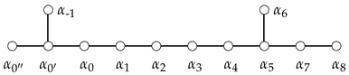
This is the extension of through the orthogonal Lie algebra .
A possible set of simple roots in the orthonormal basis of the Lorentzian space is:
where . One can realize at a glance that this is the same set of simple roots of , except for the root . We think that the possibility of discriminating between and on physical grounds can only arise when performing explicit computer calculations, which, for the case of , should undergo major simplifications due to the presence of only one irrational number, .
4. Beyond Kac–Moody
Several difficulties in proceeding with our program arise with Kac–Moody algebras:
- (P.1)
- As already mentioned above, the presence of irrational numbers in the definition of momentum variables can be very annoying in computer calculations, and it is also quite unnatural in an algebra based on integer numbers, both in the roots and in the structure constants;
- (P.2)
- The need of roots, as in item (TM.7) for , with opposite helicity and opposite signs of the three-momentum components , complicates the algebra to a large extent, since they cannot, in pairs, be roots of the Kac–Moody algebras. In the case of , this problem can be overcome by enlarging the explicit commutation relations to consistently include the new roots, but, in the case of or , one needs to further modify the Serre relations, which does not seem to be an easy task to us;
- (P.3)
- However, the most important issue comes from physics: in and , three simple roots (namely, , and ) have tachyon-like momenta due to their positive norm. The interpretation of such tachyonic momenta, as well as the investigation of their impact on the interactions among charged particles, is beyond the scope of the present paper; computer calculations, starting from an initial state, may reveal the scenario that tachyonic simple roots may yield to.
It is our opinion that these are good motivations for focusing our investigation on generalized Kac–Moody (Borcherds) algebras, where two of the three difficulties listed above disappear.
5. Borcherds
Borcherds algebras are a generalization of Kac–Moody algebras obtained by releasing the condition on the diagonal elements of the Cartan matrix, which are then allowed to be non-positive, as well as by restricting the Serre relations to the generators associated to positive norm simple roots [34,35].
A generalized Kac–Moody (or Borcherds) algebra is constructed as follows.
Let H be a real vector space with a symmetric bilinear inner product , and with elements indexed by a countable set , such that if and is an integer if is positive. The matrix A with entries is called the symmetrized Cartan matrix of .
The generalized Kac–Moody (or Borcherds) algebra associated to A is defined to be the Lie algebra generated by H and elements and , for , with the following relations:
- The (injective) image of H in is commutative;
- If h is in H, then and ;
- ;
- If and , then ad, where ;
- If , then .
If for all , then is the Kac–Moody algebra with Cartan matrix A. In general, has almost all of the properties of a Kac–Moody algebra, the only major difference being that is allowed to have imaginary simple roots.
The root lattice is the free Abelian group generated by elements for , called simple roots, and has a real-valued bilinear form defined by . The Lie algebra is then graded by with H in degree 0, (resp ) in degree (resp. ). A root is a non-zero element of such that there are elements of of degree . A root r is called real if ; otherwise, it is called imaginary. A root r is positive if it is a sum of simple roots, and negative if is positive. Notice that every root is either positive or negative, [34].
We build the following symmetrized Cartan matrix for a Borcherds algebra of rank 12, which we denote by :
Notice that, for , a four-momentum vector can be written as
Using the Cartan Matrix (50), we indeed obtain:
hence the Lorentzian scalar product:
Let us restrict to positive roots , , with , and let us denote by the corresponding subalgebra of . The physical motivation for restricting to is that, given a positive root , its four-momentum is
with , implying , namely p is either light-like or time-like. In particular:
Remark 6.
Notice that the mass of a particle cannot be arbitrarily small, since there is a lower limit .
For , , with , we introduce the notation
Thus, is in the lattice of , and a precise physical meaning is assigned to positive real and imaginary roots when :
Proposition 3.
A generator in , associated to a positive root , with and momentum , is massive if and only if is an imaginary root; it is massless if and only if r is real, in which case, it is a positive real root of .
Proof.
The proof consists of the following steps:
- From Proposition 2.1. of [34], it holds that every positive root is conjugate under the Weyl group to a root , such that either is a simple real root , , or it is a positive root in the Weyl chamber (namely for all simple roots );
- Since r and are conjugate under the Weyl group, then ;
- If is a real simple root, then it is a root of and ; is real and so is r. Since the Weyl group is generated by the reflections , where the simple roots are real, hence , it coincides with the Weyl group of . By applying to Weyl reflections, we stay within , since every Kac–Moody algebra is invariant under the Weyl group; therefore, r is a real root of , namely , and is light-like;
- If is in the Weyl chamber, then , , since all are positive, being a positive root; thus, r is imaginary;
- Since with , then , and the particle associated to r is massive.
□
Remark 7.
In the massive case, the lower limit of the mass grows with the norm of α: if is not a root of , then the mass is certainly bigger than the lower mass a particle corresponding to a root of may have. We also notice that charged massless particles ( in the root ) are quite peculiar, since their momentum can only be in one direction. The photon is not in this class, since it has , but the (non-virtual) gluons are. A non-virtual photon can be produced in a decay process [1].
6. Conclusions
In this paper, the first of a series of two papers with the same title, we have described the basic principles of a model of quantum gravity at the early stages of the universe. We have explained how spacetime is generated from an initial state and how it expands and is driven by interactions in a purely algebraic context. We have investigated the mathematical structures that may suit our purpose: they are rank-12 infinite-dimensional algebras, extending and including 4-momenta. We have also discussed why a celebrated no-go theorem on does not apply in our settings.
The companion paper [1], based on the treatment and considerations of this paper, will focus on a particular rank-12 algebra in order to build a model for quantum gravity. In particular, it will turn into a Lie superalgebra in order to fulfill the Pauli exclusion principle without producing superpartners. It will also discuss scattering processes and decays.
The algebra is based on a simplified version of a Borcherds algebra, where based on means that we still have to enlarge the algebra with roots that take into account the coupling of four momenta with those having three momenta of the opposite sign and same energy (see (P.2) of Section 4). Nothing would prevent us from starting from a Borcherds algebra, but we would not have explicit commutation relations, as we do in [1].
Author Contributions
Conceptualization, P.T., A.M., M.R. and K.I.; methodology, P.T. and A.M.; formal analysis, P.T., A.M. and M.R.; investigation, P.T.; writing—original draft preparation, P.T.; writing—review and editing, P.T., A.M. and M.R.; supervision, K.I. All authors have read and agreed to the published version of the manuscript.
Funding
This research received no external funding.
Conflicts of Interest
The authors declare no conflict of interest.
Appendix A
In this appendix, we show the charge content of the part of the algebra, root by root. Table A1 show all of the roots of , grouped by the points of the Magic Star obtained by projecting on the plane of color , see Section 2.2. The leptons, being colorless, lie in the center of this Magic Star, forming the roots of Table A2. In addition, the roots of this lie on a Magic Star (of a smaller dimension) once projected on the plane of flavor . The families of leptons and quarks are shown in Table A3 and Table A4, together with their spin. For the quarks sector, we only consider one color, which we name blue; similar tables for red and green colors are trivially obtained by exchanging indices.

Table A1.
The Magic Star of ; ; , .
| Roots | # | |||
|---|---|---|---|---|
| 0 | 2 | |||
| 0 | 2 | |||
| 0 | 2 | |||
| 0 | 24 | |||
| 1 | 8 | |||
| 8 | ||||
| 0 | 16 | |||
| 1 | 8 | |||
| 8 | ||||
| 2 | ||||
| 1 | ||||
| 8 | ||||
| 8 | ||||
| - | 8 | |||
| 2 | ||||
| 1 | ||||
| 8 | ||||
| 8 | ||||
| 8 | ||||
| 2 | ||||
| 1 | ||||
| 8 | ||||
| 8 | ||||
| 8 | ||||
| 2 | ||||
| 1 | ||||
| 8 | ||||
| - | 8 | |||
| 8 | ||||
| 2 | ||||
| 1 | ||||
| 8 | ||||
| 8 | ||||
| 8 | ||||
| 2 | ||||
| 1 | ||||
| 8 | ||||
| - | 8 | |||
| 8 |
Table A2.
The Magic Star of ; ; , .
| Roots | ||||
|---|---|---|---|---|
| 2 | ||||
| 0 | 2 | |||
| 2 | ||||
| 0 | 4 | |||
| 0 | 4 | |||
| 1 | 2 | |||
| 2 | ||||
| 0 | 1 | |||
| 1 | 4 | |||
| 0 | 2 | |||
| 1 | 2 | |||
| 0 | 1 | |||
| 4 | ||||
| 2 | ||||
| 0 | 2 | |||
| 1 | ||||
| 0 | 4 | |||
| 2 | ||||
| 0 | 2 | |||
| 1 | 1 | |||
| 0 | 4 | |||
| 0 | 2 | |||
| 1 | 2 | |||
| 1 | ||||
| 0 | 4 | |||
| 2 | ||||
| 0 | 2 | |||
| 1 | 1 | |||
| 0 | 4 | |||
| 0 | 2 | |||
| 1 | 2 |
Table A3.
The lepton families with their spin-z.
| 0 | ||||
| 0 | ||||
| 1 | ||||
| 1 | ||||
| 0 | 1/2 | |||
| 0 | 1/2 | |||
| 1/2 | ||||
| 1/2 | ||||
| 1/2 | ||||
| 1/2 | ||||
| 0 | 1/2 | |||
| 0 | 1/2 | |||
| 1 | ||||
| 1 | ||||
| 0 | ||||
| 0 | ||||
| 0 | ||||
| 0 | ||||
| 1 | 1/2 | |||
| 1 | 1/2 | |||
| 0 | 1/2 | |||
| 0 | 1/2 | |||
| 0 | ||||
| 0 | ||||
| 1 | 1/2 | |||
| 1 | 1/2 | |||
| 0 | 1/2 | |||
| 0 | 1/2 |
Table A4.
The flavor families of blue ({1,1}) quarks with their spin-z.
| u | ||||
| c | ||||
| t | ||||
| T | ||||
| t | ||||
| T | ||||
| c | ||||
| u | ||||
References
- Truini, P.; Marrani, A.; Rios, M.; Irwin, K. Space, Matter and Interactions in a Quantum Early Universe. Part II: Superalgebras and Vertex Algebras. arXiv 2012, arXiv:2012.10248. [Google Scholar] [CrossRef]
- Distler, J.; Garibaldi, S. There is no “theory of everything” inside e8. Comm. Math. Phys. 2010, 298, 419–436. [Google Scholar] [CrossRef] [Green Version]
- Belavin, A.A.; Polyakov, A.M.; Zamolodchikov, A.B. Infinite conformal symmetry in two-dimensional quantum field theory. Nucl. Phys. B 1984, 241, 333–380. [Google Scholar] [CrossRef] [Green Version]
- Dijkgraaf, R.; Vafa, C.; Verlinde, E.; Verlinde, H. The operator algebra of orbifold models. Comm. Math. Phys. 1989, 123, 485–526. [Google Scholar] [CrossRef]
- Huang, Y.-Z.; Lepowsky, J. Toward a theory of tensor products for representations of a vertex operator algebra. In Proceedings of the 20th International Conference on Differential Geometric Methods in Theoretical Physics, New York, NY, USA, 12–15 September 1991; Catto, S., Rocha, A., Eds.; World Scientific: Singapore, 1992; Volume 1, pp. 344–354. [Google Scholar]
- Borcherds, R.E. Vertex algebras, Kac–Moody algebras, and the Monster. Proc. Natl. Acad. Sci. USA 1986, 83, 3068–3071. [Google Scholar] [CrossRef] [Green Version]
- Frenkel, I.; Lepowsky, J.; Meurman, A. Vertex operator algebras and the Monster. In Pure and Applied Mathematics; Academic Press: Cambridge, MA, USA, 1988; Volume 134. [Google Scholar]
- Kac, V.G. Vertex algebras for beginners. In University Lecture Series, 2nd ed.; American Mathematical Society: Providence, RI, USA, 1998; Volume 10. [Google Scholar]
- Conway, J.H.; Norton, S.P.; Simon, P. Monstrous Moonshine. Bull. London Math. Soc. 1979, 11, 308–339. [Google Scholar] [CrossRef]
- Freidel, L.; Perez, A.; Pranzetti, D. The loop gravity string. Phys. Rev. 2017, D95, 106002. [Google Scholar] [CrossRef] [Green Version]
- Freidel, L.; Livine, E.R.; Pranzetti, D. Gravitational edge modes: From Kac–Moody charges to Poincaré networks. Class. Quant. Grav. 2019, 36, 195014. [Google Scholar] [CrossRef] [Green Version]
- Tumanov, A.G.; West, P. E11 in 11D. Phys. Lett. 2016, B758, 278. [Google Scholar] [CrossRef] [Green Version]
- Sheppeard, M.D. Constraining the Standard Model in Motivic Quantum Gravity. In Proceedings of the 32nd International Colloquium on Group Theoretical Methods in Physics (Group32), Prague, Czech Republic, 9–13 July 2018. [Google Scholar]
- Arkani-Hamed, N.; Trnka, J. The Amplituhedron. arXiv 2014, arXiv:1312.2007. [Google Scholar] [CrossRef] [Green Version]
- Mizera, S. Combinatorics and topology of Kawai-Lewellen-Tye relations. arXiv 2017, arXiv:1706.08527. [Google Scholar] [CrossRef] [Green Version]
- Arkani-Hamed, N.; Bai, Y.; Lam, T.J. Positive Geometries and Canonical Forms. arXiv 2017, arXiv:1703.04541. [Google Scholar] [CrossRef] [Green Version]
- Stasheff, J.D. Homotopy associativity of H-spaces. I; II. Trans. Am. Math. Soc. 1963, 108, 275–292. [Google Scholar] [CrossRef]
- Stasheff, J.D. From operads to physically inspired theories, Operads: Proceedings of Renaissance Conferences (Hartford, CT/Luminy, 1995). Contemp. Math. 1997, 202, 53–81. [Google Scholar]
- Tonks, A. Relating the associahedron and the permutohedron, Operads: Proceedings of Renaissance Conferences (Hartford, CT/Luminy, 1995). Contemp. Math. 1997, 202, 33–36. [Google Scholar]
- Loday, J.L. Realization of the Stasheff polytope. Arch. Math. 2004, 83, 267. [Google Scholar] [CrossRef] [Green Version]
- Senechal, M.L. Quasicrystals and Geometry; Cambridge University Press: Cambridge, UK, 1995. [Google Scholar]
- Sadoc, J.; Mosseri, R. The e8 lattice and quasicrystals. J. Non-Crystalline Solids 1993, 153, 247–252. [Google Scholar] [CrossRef]
- Fang, F.; Hammock, D.; Irwin, K. Methods for Calculating Empires in Quasicrystals. Crystals 2017, 7, 304. [Google Scholar] [CrossRef] [Green Version]
- Carter, R.W. Simple Groups of Lie Type; Wiley-Interscience: New York, NY, USA, 1989. [Google Scholar]
- Humphreys, J.E. Introduction to Lie Algebras and Representation Theory; Springer: New York, NY, USA, 1972. [Google Scholar]
- de Graaf, W.A. Lie Algebras: Theory and Algorithms; North-Holland Mathematical Library 56; Elsevier: Amsterdam, The Netherlands, 2000. [Google Scholar]
- Kac, V.G. Infinite Dimensional Lie Algebras, 3rd ed.; Reprinted with Corrections; Cambridge University Press: Cambridge, UK, 1995. [Google Scholar]
- Truini, P. Exceptional Lie Algebras, SU(3) and Jordan Pairs. Pac. J. Math. 2012, 260, 227. [Google Scholar] [CrossRef] [Green Version]
- Loos, O. Jordan Pairs; Lect. Notes Math. 460; Springer: Berlin/Heidelberg, Germany, 1975. [Google Scholar]
- Truini, P.; Biedenharn, L.C. An E6⊗U(1) invariant quantum mechanics for a Jordan pair. J. Math. Phys. 1982, 23, 1327–1345. [Google Scholar] [CrossRef]
- Marrani, A.; Truini, P. Exceptional Lie Algebras, SU(3) and Jordan Pairs, Part 2: Zorn-type Representations. J. Phys. 2014, A47, 265202. [Google Scholar] [CrossRef] [Green Version]
- Moody, R.V. A new class of Lie algebras. J. Algebra 1968, 10, 211–230. [Google Scholar] [CrossRef] [Green Version]
- Fuchs, J. Lectures on conformal field theory and Kac–Moody algebras. In Conformal Field Theories and Integrable Models; Horváth, Z., Palla, L., Eds.; Lecture Note Physic 498; Springer: Berlin/Heidelberg, Germany, 1997. [Google Scholar]
- Borcherds, R.E. Generalized Kac–Moody algebras. J. Algebra 1988, 115, 501–512. [Google Scholar] [CrossRef] [Green Version]
- Borcherds, R.E. Monstrous moonshine and monstrous Lie superalgebras. Invent. Math. 1992, 109, 405–444. [Google Scholar] [CrossRef] [Green Version]
Figure 1.
Expansion of a particle (blue dot) along (x-axis) with amplitudes (y-axis).
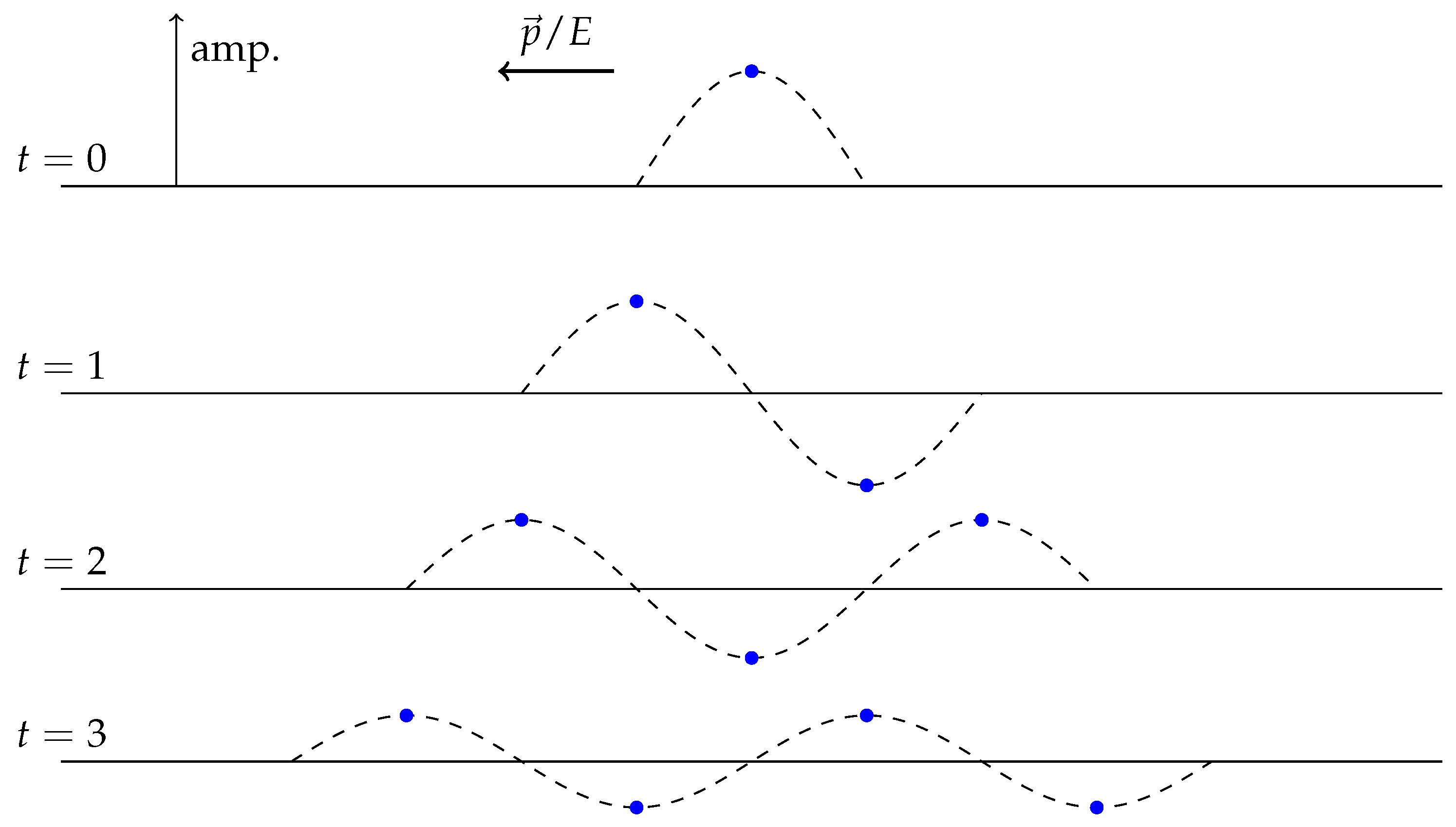
Figure 2.
The Magic Star (MS): in the MS of , in the MS of ; the triangles represent the and representations of the with roots in the external hexagon.
Figure 2.
The Magic Star (MS): in the MS of , in the MS of ; the triangles represent the and representations of the with roots in the external hexagon.
Publisher’s Note: MDPI stays neutral with regard to jurisdictional claims in published maps and institutional affiliations. |
© 2021 by the authors. Licensee MDPI, Basel, Switzerland. This article is an open access article distributed under the terms and conditions of the Creative Commons Attribution (CC BY) license (https://creativecommons.org/licenses/by/4.0/).
Share and Cite
MDPI and ACS Style
Truini, P.; Marrani, A.; Rios, M.; Irwin, K. Space, Matter and Interactions in a Quantum Early Universe Part I: Kac–Moody and Borcherds Algebras. Symmetry 2021, 13, 2342. https://doi.org/10.3390/sym13122342
AMA Style
Truini P, Marrani A, Rios M, Irwin K. Space, Matter and Interactions in a Quantum Early Universe Part I: Kac–Moody and Borcherds Algebras. Symmetry. 2021; 13(12):2342. https://doi.org/10.3390/sym13122342
Chicago/Turabian StyleTruini, Piero, Alessio Marrani, Michael Rios, and Klee Irwin. 2021. "Space, Matter and Interactions in a Quantum Early Universe Part I: Kac–Moody and Borcherds Algebras" Symmetry 13, no. 12: 2342. https://doi.org/10.3390/sym13122342
Note that from the first issue of 2016, this journal uses article numbers instead of page numbers. See further details here.