Reconstruction of Scalar-Torsion Gravity Theories from the Physical Potential of a Scalar Field

Abstract

We consider scalar-torsion gravity theories based on the exact solutions of a physical type of potential for cosmological inflationary models based on the non-minimal coupling of a scalar field and torsion. We analyzed the inflationary models with different types of inflationary dynamics and corresponding scalar field parameters. Such an approach allows us to consider different physical potentials and types of scalar-torsion gravity theories in the context of the realization of both stages of accelerated expansion of the universe. We also considered the correspondence surrounding the proposed inflationary models and the observational constraints on the parameters of cosmological perturbations.

1. Introduction

Scalar field cosmology has been actively exploited in inflation (since the beginning of its introduction) [1]. Single scalar fields with various types of potentials have been considered in studies concerning early and later inflation [1,2].

Understanding the physical processes at the early stages of the evolution of the universe involves an approximate analysis of cosmological dynamics in the slow-roll regime [3]. Moreover, exact solutions have been used to construct and analyze the inflationary models; see [2,4].

To explain the early inflationary and late time-accelerated expansion of the universe, various modified theories of gravity are being considered [5,6,7,8]. One such approach is the teleparallel equivalent of general relativity (TEGR), in which the torsion is used instead of the scalar curvature to describe the gravitational interaction [9,10,11] and its various modifications, such as $f\left(T\right)$-gravity [12,13,14,15,16]. Cosmological models based on non-minimal coupling between the scalar field and torsion [17,18,19,20,21,22] and other modifications of TEGR [23,24,25,26], including non-canonical kinetic terms [27], are also considered to construct and analyze cosmological models.

Torsion can be considered a dynamic degree of freedom in the framework of quantum gravity [28,29], i.e., non-zero torsion must be taken into account when analyzing cosmological models based on quantum cosmology [30,31,32,33,34].

Although the effects of the non-zero torsion of space–time have not been detected, various methods for detecting such effects have been proposed, for example, by the spectra of gravitational waves from astrophysical sources [35,36] or by possible small deviations of the motion of the Moon and Mercury from GR predictions for non-zero torsion [37,38].

In the framework of teleparallel gravity, gravitational interaction is described in terms of torsion; the tetrad field instead of the metric tensor is a dynamic variable and the usual Levi–Civita connection (without torsion in the framework of GR) is replaced with the Weizenbeck connection, which implies non-zero torsion rather than curvature [9,10,11]. Although the equations of the gravitational field are the same in both cases (TEGR and GR), in contrast to Einstein’s gravity, teleparallel gravity is a gauge theory of gravity [9,10,11].

Differences between these two approaches to the description of the gravitational interaction also appear when considering their expansion, taking into account the non-minimal coupling between the scalar field and curvature [39,40] or torsion [17,18,19,20,21,22].

In the case of the scalar-tensor theories of gravity, the initial action can be reduced to the Einstein–Hilbert action through conformal transformations of the space–time metric and material components [39,40]. In the case of teleparallel gravity, the non-minimal coupling of the field with torsion cannot be eliminated through conformal transformations, i.e., the models based on scalar-torsion gravity theories have no analogs in the framework of the teleparallel gravity with minimal coupling [41,42,43].

In the absence of such conformal transformations, an approach based on the determination of parametric and functional relationships (the PFR approach) between model parameters with non-minimal coupling and minimal coupling of the scalar field and torsion seems to be productive for the analysis of cosmological models based on the scalar-torsion gravity.

This approach was previously considered in references [44,45,46,47,48] for the analysis of cosmological models with non-minimal coupling between the scalar field and the Gauss–Bonnet scalar; this PFR approach was also applied to the case of cosmological models based on scalar-tensor gravity theories [49,50,51,52,53].

Within the framework of this PFR approach, the influence of the non-minimal coupling of the scalar field and curvature (and the Gauss–Bonnet term) was considered based on certain relationships between the parameters of cosmological models with the on-minimal and minimal coupling of the Friedman–Robertson–Walker space–time background concerning background cosmological dynamics and the parameters of cosmological perturbations. In this case, the problem with the correspondence of cosmological models to the observational constraints on the parameters of cosmological perturbations [54,55] is reduced to determining the values of the model’s constants for arbitrary models [48,53].

In this paper, we consider the application of this PFR approach to the problems of constructing and analyzing the models of cosmological inflation based on scalar-torsion gravity theories with non-minimal coupling between the scalar field and torsion. The work is organized as follows. Section 2 deals with the equations of cosmological dynamics and their properties for inflationary models based on the scalar-torsion theory of gravity. Only two of the three equations are independent, and any two of them can be used to fully describe the cosmological dynamics. Section 3 proposes the description of cosmological models based on the teleparallel equivalent of the general theory of relativity (TEGR). In Section 4, we consider the cosmological models based on scalar-torsion gravity with the power–law parametric connection between the Hubble parameter and coupling function $F\sim H^n$ and formulate the conditions to construct phenomenological correct cosmological models, which satisfy the modern observational data. Moreover, we consider two classes of exact solutions (generalized and special ones) of cosmological dynamic equations for these models. In Section 5, we consider the parameters of cosmological perturbations for inflationary models based on scalar-torsion gravity with the power–law connection $F\sim H^n$ and compare them with the ones in the models based on TEGR. In Section 6, we reconstruct scalar-torsion gravity theories based on the physical potential of a scalar field. The basis of this approach is the verification of a cosmological inflationary model with physical potential that does not meet the observational constraints for the TEGR case. Modification of the gravity theory makes it possible to verify inflationary models in accordance with observational data. Scalar-torsion gravity obtained by this method corresponds to a non-minimal coupling for a small field. Finally, Section 7 presents our summary.

2. Cosmological Models Based on the Scalar-Torsion Gravity

The action for cosmological models based on scalar-torsion gravity can be written as follows [20,21,22]

$$S=\int d^{4}xe\left[-\frac{1}{2}F\left(\varphi \right)T-\frac{1}{2}\omega \left(\varphi \right){\partial }_{\mu }\varphi {\partial }^{\mu }\varphi -V\left(\varphi \right)\right],$$

(1)

where $e=det\left(e_{\mu }^A\right)=\sqrt{-g}$, $e_{\mu }^A$ is the tetrad field, $F\left(\varphi \right)$ is a coupling function between the scalar field $\varphi$ and torsion scalar T, $\omega \left(\varphi \right)$ is a kinetic function and $V\left(\varphi \right)$ is the potential of a scalar field.

The diagonal tetrad field

$$e_{\mu }^A=\mathrm{diag}(1,a,a,a),$$

(2)

corresponds to the flat Friedmann–Robertson–Walker (FRW) metric

$$d{s}^2=-d{t}^2+a^2{\delta }_{ij}d{x}^{i}d{x}^j,$$

(3)

where $a=a\left(t\right)$ is the scale factor and t is the cosmic time.

The background equations corresponding to the action (1) for the flat FRW metric (3) are [20,21,22]

$$E_1\equiv 3H^{2}F-\frac{1}{2}\omega {\dot{\varphi }}^2-V\left(\varphi \right)=0,$$

(4)

$$E_2\equiv 3H^{2}F+\frac{1}{2}\omega {\dot{\varphi }}^2-V\left(\varphi \right)+2H\dot{F}+2F\dot{H}=0,$$

(5)

$$E_3\equiv \omega \ddot{\varphi }+3\omega H\dot{\varphi }+\frac{1}{2}{\dot{\varphi }}^2{\omega }^{\prime }+3H^2{F}^{\prime }+V^{\prime }=0,$$

(6)

where an overdot represents a derivative with respect to the cosmic time t, $H\equiv \dot{a}/a$ denotes the Hubble parameter and the torsion scalar is connected with the Hubble parameter as $T=6H^2$ and $F^{\prime }\equiv \partial F/\partial \varphi$.

First, by direct substitution, one can check that Equations (4)–(6) are connected by the relation

$$\dot{\varphi }{E}_3+{\dot{E}}_1+3H\left(E_1-E_3\right)=0,$$

(7)

similar to the case of the scalar-tensor gravity [49,50,51,52,53].

However, we note that the equations of cosmological dynamics (4)–(6) themselves differ from the equations of dynamics for the scalar-tensor gravity case, which contains additional terms [49,50,51,52,53].

Thus, there are only two independent equations in this system, and one can consider any two equations that completely describe the cosmological dynamics.

3. Cosmological Models with Minimal Coupling $\mathit{F}=\mathbf{1}$

For the case of minimal coupling $F=1$, scalar-torsion gravity is reduced to the teleparallel equivalent of general relativity (TEGR).

For TEGR, under conditions $F=1$ and $\omega =1$, dynamic Equations (4)–(6) are reduced to

$$3H^2=\frac{1}{2}{\dot{\varphi }}^2+V\left(\varphi \right),$$

(8)

$$-3H^2-2\dot{H}=\frac{1}{2}{\dot{\varphi }}^2-V\left(\varphi \right),$$

(9)

$$\ddot{\varphi }+3H\dot{\varphi }+V^{\prime }=0,$$

(10)

which also correspond to the case of inflationary models based on general relativity [1,2].

In this system of equations, the two equations are independent; moreover, we can represent the equations, which define the dynamics of the early universe as [2]

$$V\left(\varphi \right)=3H^2+\dot{H},$$

(11)

$$X=\frac{1}{2}{\dot{\varphi }}^2=-\dot{H}.$$

(12)

One can also use the condition of minimal coupling $F=1$ only and redefine the scalar field in Equations (4)–(6) as $\phi =\int \sqrt{\omega \left(\varphi \right)}d\varphi$, which leads to the same Equations (8)–(10) in terms of a new scalar field $\phi$.

For analyses of such models, including the exact solutions, construction, and analysis of the cosmological perturbations, see, for example, [2].

We also consider compliance with the conditions for the scalar field to slowly roll down to the minimum of the potential, which implies the predominance of the potential over the kinetic energy $X\ll V$ for the accelerated expansion of the early universe at the inflationary stage.

Now, we define the reduced potential $\tilde{V}$ and reduced kinetic energy $\tilde{X}$ as follows

$$\tilde{V}=\frac{V}{H^2}=3-ϵ,$$

(13)

$$\tilde{X}=\frac{X}{H^2}=ϵ,$$

(14)

where $ϵ=-\frac{\dot{H}}{H^2}$ is the slow-roll parameter.

Under conditions of the quasi-de Sitter-accelerated expansion of the early universe $ϵ\ll 1$, from (13) and (14), we obtain $\tilde{X}\ll \tilde{V}$ and $X\ll V$. Thus, slow-roll conditions are satisfied for inflationary models based on TEGR (similar to the case of GR) when $ϵ\ll 1$.

Thus, the analysis of the equations of cosmological dynamics based on TEGR corresponds to the case of general relativity.

4. Cosmological Models with Non-Minimal Coupling $\mathit{F}\ne \mathit{const}$

To analyze the cosmological models under consideration, we represent the first two equations of systems (4)–(6) in the following form

$$V\left(\varphi \right)=3H^{2}F+\frac{d}{dt}\left(FH\right),$$

(15)

$$X=\frac{1}{2}\omega \left(\varphi \right){\dot{\varphi }}^2=-\frac{d}{dt}\left(FH\right).$$

(16)

For minimal coupling, $F=1$ and $\omega =1$ expressions (15) and (16) are reduced to dynamic Equations (11) and (12) for TEGR.

Now, we rewrite Equations (15) and (16) in terms of the generating function

$$G\left(t\right)\equiv H\left(t\right)F\left(t\right),$$

(17)

as follows

$$V\left(\varphi \right)=3HG+\dot{G},$$

(18)

$$X=\frac{1}{2}\omega \left(\varphi \right){\dot{\varphi }}^2=-\dot{G}.$$

(19)

Thus, to analyze cosmological models based on scalar-torsion gravity, it is necessary to consider a special form of the generating function G.

For the case $F=1$ from (17), we obtain $G=H$, and dynamic Equations (18) and (19) are reduced to (11) and (12) for TEGR.

4.1. The Special Kind of the Generating Function

In the general case, one can analyze models of cosmological inflation based on scalar-torsion gravity for an arbitrary function $G=G\left(t\right)$.

Nevertheless, we are interested in the parametrization of the influence of the non-minimal coupling between torsion and the scalar field, which must also imply the fulfillment of the slow-roll conditions on the inflationary stage and the reduction of the model to the de Sitter one for the case of the minimal coupling $F=1$ (the cosmological models based on this approach for the scalar-tensor gravity theories with non-minimal coupling between the scalar field and curvature were considered earlier in [49,50,51,52,53]).

To satisfy these requirements, we consider the following generating function

$$\begin{array}{ccc}\hfill & & G\left(H\right)=\frac{1}{{\lambda }^n}{H}^{n+1},\hfill \end{array}$$

(20)

with the corresponding power–law connection between the coupling function and the Hubble parameter

$$\begin{array}{ccc}\hfill & & F\left(\varphi \left(t\right)\right)={\left(\frac{H\left(t\right)}{\lambda }\right)}^n,\hfill \end{array}$$

(21)

where $\lambda$ and n are some constants.

After the substitution of the connection (21) into Equations (15) and (16), we obtain

$$V\left(\varphi \right)=\frac{H^n}{{\lambda }^n}\left[3H^2+(n+1)\dot{H}\right],$$

(22)

$$X(\varphi ,\dot{\varphi })\equiv \frac{1}{2}\omega \left(\varphi \right){\dot{\varphi }}^2=-\frac{H^n}{{\lambda }^n}\left(n+1\right)\dot{H}.$$

(23)

Let us analyze the system (21)–(23) for different values of the parameter n, namely:

• For $n=0$, one has $F=1$, and Equations (22) and (23) are reduced to (11) and (12) for the minimal coupling (TEGR).
• For $n\ne 0$ and $F=1$, one has $H=\lambda =const$, $a\left(t\right)\sim exp\left(\lambda t\right)$, $V=3{\lambda }^2$, and $X=0$. These solutions correspond to the de Sitter stage for TEGR, where the pure exponential expansion of the universe is induced by the cosmological constant $\Lambda =V=3{\lambda }^2$.
• For $n\ne 0$ and $F=F\left(t\right)\ne const$, one has cosmological models based on scalar-torsion gravity, which is reduced to the de Sitter solutions coinciding with the case of TERG for $H=\lambda =const$.

Thus, for the models based on the power–law connection between the coupling function and the Hubble parameter (21) with $n\ne 0$, the non-minimal coupling between the torsion and scalar field induces the deviations of cosmological dynamics from the pure exponential expansion, the deviations of the potential from the flat one, and the evolution of the scalar field itself.

Now, we define the reduced potential $\tilde{V}$ and reduced kinetic energy $\tilde{X}$ as follows

$$\tilde{V}=\frac{{\lambda }^n}{H^{n+2}}V=3-(n+1)ϵ,$$

(24)

$$\tilde{X}=\frac{{\lambda }^n}{H^{n+2}}X=(n+1)ϵ.$$

(25)

Under the quasi-de Sitter accelerated expansion of the early universe $ϵ\ll 1$, from (24) and (25) we obtain $\tilde{X}\ll \tilde{V}$, and $X\ll V$ for $|n+1|ϵ\ll 1$.

Thus, the slow-roll conditions for the inflationary models based on scalar-torsion gravity with the power–law connection (21) between the coupling function and the Hubble parameter are similar to TEGR under condition $|n+1|\sim 1$.

4.2. The Conditions of the Non-Minimal Coupling Function

We also consider the following condition on the coupling function

$$\begin{array}{ccc}\hfill & & F(t\to \infty )=1,\hfill \end{array}$$

(26)

i.e., we will consider inflationary models, which are reduced to the TEGR models with cosmological constants at large times.

This condition first allows one to explain the second accelerated expansion of the universe at large times within the framework of the $\Lambda$CDM model [56], since under condition (26) the models under consideration are reduced to the $\Lambda$CDM model with a cosmological constant

$$\begin{array}{ccc}\hfill & & \Lambda =V=3{\lambda }^2=const.,\hfill \end{array}$$

(27)

and taking into account the other material fields at large times, namely baryonic and dark matter, we obtain the $\Lambda$CDM model, which has good correspondence with modern observational data [57,58].

Secondly, we can consider a wide class of generalized models of scalar-torsion gravity with arbitrary coupling $F=F\left(\varphi \right)$ and kinetic $\omega =\omega \left(\varphi \right)$ functions at the inflationary stage, taking into account condition (26), since at large times, such models will be reduced to TEGR, satisfying the modern observational tests, similar to GR [59].

4.3. General Exact Solutions of the Dynamic Equations

Since the accelerated expansion of the early universe and conditions (21) and (26) restrict the possible types of inflationary dynamics, we will determine the Hubble parameter $H=H\left(t\right)$ to construct and analyze the cosmological models.

Using the following expression,

$$\begin{array}{c}\hfill \dot{\varphi }=\frac{d\varphi }{dH}\frac{dH}{dt}={\left(\frac{dH}{d\varphi }\right)}^{-1}\dot{H},\end{array}$$

(28)

from (21)–(23) we obtain the parameters of inflationary models

$$V\left(\varphi \right)=\frac{H^n}{{\lambda }^n}\left[3H^2+(n+1)\dot{H}\right],$$

(29)

$$\omega \left(\varphi \right)=-2{\left(\frac{H}{\lambda }\right)}^n{\left(\frac{dH}{d\varphi }\right)}^2\left(\frac{n+1}{\dot{H}}\right),$$

(30)

$$F\left(\varphi \right)={\left(\frac{H\left(\varphi \right)}{\lambda }\right)}^n,$$

(31)

with two additional equations

$$\dot{H}=\dot{H}\left(H\right),$$

(32)

$$H\left(\varphi \right)=H\left(t\right).$$

(33)

Thus, for the chosen Hubble parameter as a function of cosmic time $H=H\left(t\right)$, one can define dependence (32) in explicit form, and for the chosen Hubble parameter as a function of the scalar field $H=H\left(\varphi \right)$, one can obtain the evolution of the scalar field $\varphi =\varphi \left(t\right)$ from Equation (33) and reconstruct the potential of a scalar field $V\left(\varphi \right)$ and the parameters of scalar-torsion gravity from expressions (29)–(31) as well.

4.4. Special Class of Exact Solutions of Dynamic Equations

We also consider the special class of exact cosmological solutions implying the same scalar field evolution $\varphi =\varphi \left(t\right)$ and the Hubble parameter $H=H\left(t\right)$ for TERG and scalar-torsion gravity under consideration

$$\begin{array}{ccc}\hfill & & \varphi ={\varphi }_{TEGR},H=H_{TEGR},V\ne V_{TEGR}.\hfill \end{array}$$

(34)

In this case, the non-minimal coupling scalar field with torsion changes its potential only, i.e., it affects the character of realization of the inflationary stage for the models of the early universe under consideration.

With this aim, we consider the following kinetic function

$$\begin{array}{ccc}\hfill & & \omega \left(\varphi \right)=\frac{H^n}{{\lambda }^n}(n+1)=(n+1)F\left(\varphi \right).\hfill \end{array}$$

(35)

In this case, Equations (22) and (23) are reduced to

$$V\left(\varphi \right)=\frac{H^n}{{\lambda }^n}\left[3H^2+(n+1)\dot{H}\right],$$

(36)

$$\frac{1}{2}{\dot{\varphi }}^2=-\dot{H},$$

(37)

where the second equation is the same as the one for TERG (12), however, the potential is different from one for TERG (11).

5. The Parameters of Cosmological Perturbations

In accordance with the theory of cosmological perturbations, quantum fluctuations of the scalar field induce the corresponding perturbations of the space–time metric during the inflationary stage. In the linear order of the cosmological perturbation theory, the observed anisotropy and polarization of the cosmic microwave background radiation (CMB) [1,2] are explained by the influences of two types of perturbations—scalar and tensor.

Observational constraints on the parameters of cosmological perturbations due to the modern observations of the anisotropy and polarization of CMB are [54,55]

$$P_S=2.1\times {10}^{-9},$$

(38)

$$n_S=0.9663\pm 0.0041,$$

(39)

$$r<0.032.$$

(40)

The cosmological perturbation parameters for inflationary models (based on scalar-torsion gravity for an arbitrary type of coupling between the scalar field and torsion) were considered early; see [21].

When the slow-roll conditions are satisfied, the expressions for the parameters of cosmological perturbations on the crossing of the Hubble radius ($k=aH$) for the models with the power–law connection (21), due to results obtained in [21], can be written as follows

$${\mathcal{P}}_S=\frac{H^2}{8{\pi }^2{Q}_S}=-\frac{H^4}{8{\pi }^2\dot{G}},$$

(41)

$${\mathcal{P}}_T=\frac{H^2}{2{\pi }^2{Q}_T}=\frac{2H^2}{{\pi }^{2}F},$$

(42)

$$n_S-1=-2ϵ-\frac{{\dot{Q}}_S}{H{Q}_S}=-4ϵ-\frac{\ddot{G}}{H\dot{G}}=-4ϵ+2{\delta }_{ST},$$

(43)

$$r=\frac{{\mathcal{P}}_T}{{\mathcal{P}}_S}=4\frac{Q_S}{Q_T}=16\left(ϵ-\frac{\dot{F}}{HF}\right)=-16\left(\frac{\dot{G}}{HG}\right)=16{ϵ}_{ST},$$

(44)

where

$$Q_S=\frac{\omega X}{H^2}=-\frac{1}{H^2}\frac{d}{dt}\left(FH\right)=-\frac{\dot{G}}{H^2},Q_T=\frac{1}{4}F,$$

(45)

$${ϵ}_{ST}=-\frac{\dot{G}}{HG},{\delta }_{ST}=-\frac{\ddot{G}}{2H\dot{G}},$$

(46)

and we define the new slow-roll parameters (${ϵ}_{ST}$ and ${\delta }_{ST}$) for inflationary models based on scalar-torsion gravity, reduced to the usual ones, i.e., ${ϵ}_{ST}\to ϵ$ and ${\delta }_{ST}\to \delta$ for the cases involving minimal coupling ($F=1$ and $G=H$).

Thus, the slow-roll conditions for inflationary models based on action (1) can be formulated as follows

$$\begin{array}{ccc}\hfill & & ϵ\ll 1,{ϵ}_{ST}\ll 1,{\delta }_{ST}\ll 1,\hfill \end{array}$$

(47)

which restrict possible types of the Hubble parameter $H=H\left(t\right)$ and generate function $G=FH$.

Moreover, the values of the parameters of cosmological perturbations do not depend on the type of the kinetic function $\omega =\omega \left(\varphi \right)$.

To compare the predictions of the inflationary model with the observational data of CMB anisotropy, two parameters of cosmological perturbations should be considered, namely, the spectral index of scalar perturbations $n_S$ and the tensor–scalar ratio r if one can obtain the dependence $r=r\left(n_S\right)$ in explicit form (since the condition (38) can always be met by choosing the model’s constant parameters).

5.1. The Case of Inflationary Models Based on TEGR

For the case of minimal coupling $F=1$, one has $G=H$, ${ϵ}_{ST}=ϵ$, ${\delta }_{ST}=\delta$ and expressions (41)–(44) for parameters of cosmological perturbations are reduced to well-known ones

$${\mathcal{P}}_S=-\frac{H^4}{8{\pi }^2\dot{H}}=\frac{1}{2ϵ}{\left(\frac{H}{2\pi }\right)}^2,$$

(48)

$$n_S-1=-4ϵ+2\delta ,$$

(49)

$$r=\frac{{\mathcal{P}}_T}{{\mathcal{P}}_S}=16ϵ,$$

(50)

where

$$\begin{array}{ccc}\hfill & & \delta =-\frac{\ddot{H}}{2H\dot{H}}\ll 1,\hfill \end{array}$$

(51)

is the second slow-roll parameter.

Thus, parameters of cosmological perturbations for inflationary models based on TEGR are the same as ones for the case of general relativity [1,2].

5.2. Inflationary Models Based on Scalar-Torsion Gravity with Connection $F\sim H^n$

From the definition of the slow-roll parameters (46) for the generating function (20), one has

$${ϵ}_{ST}=-(n+1)\frac{\dot{H}}{H^2}=(n+1)ϵ,$$

(52)

$${\delta }_{ST}=-\frac{n}{2}\frac{\dot{H}}{H^2}-\frac{\ddot{H}}{2H\dot{H}}=\frac{n}{2}ϵ+\delta .$$

(53)

Thus, slow-roll conditions are satisfied for the models with a power–law connection between the Hubble parameter and the coupling function (21), when $\left|n\right|ϵ\ll 1$ and $\delta \ll 1$.

After substituting (52) and (53) into (41)–(44), we obtain

$${\mathcal{P}}_S=\frac{{\lambda }^n}{2(n+1)ϵ}{\left(\frac{H}{2\pi }\right)}^2,$$

(54)

$$n_S-1=(n-4)ϵ+2\delta ,$$

(55)

$$r=\frac{{\mathcal{P}}_T}{{\mathcal{P}}_S}=16(n+1)ϵ,$$

(56)

where from Equation (56) one has the following restriction on the constant parameter $n>-1$ when taking into account the condition $ϵ\ge 0$.

Since the parameters of cosmological perturbations are determined based on the Hubble parameter $H=H\left(t\right)$ only, the parameters of cosmological perturbations for the case of general (28)–(33) and special (35)–(37) exact solutions of cosmological dynamics equations will be the same for the same Hubble parameter.

For case $n=0$, expressions (54)–(56) for the parameters of cosmological perturbations for non-minimal coupling are reduced to (48)–(50) for minimal coupling.

This result allows us to estimate the value of the parameter n for different inflationary models, using observational constraints on the values of parameters of cosmological perturbations.

6. Cosmological Models Based on Scalar-Torsion Gravity with Connection $\mathit{F}\sim {\mathit{H}}^{\mathit{n}}$

Now, we consider the inflationary models based on scalar-torsion gravity with the power–law connection between the coupling function and the Hubble parameter (21). In this case, we are more interested in a special class of exact cosmological solutions to illustrate the influence of the non-minimal coupling of the scalar field and torsion on the potential of the scalar field and the parameters of cosmological perturbations. For these purposes, we consider models of cosmological inflation that do not comply with the observational constraints on the values of the parameters of cosmological perturbations. In this case, the observational constraints will be interpreted as conditions on the parameters of reconstructed scalar-torsion gravity models.

Nevertheless, we note that similar constraints can be used in the analysis of scalar-torsion gravity models obtained based on generalized solutions of the equations of cosmological dynamics.

6.1. The Hyperbolic Inflationary Model

First, we consider the inflationary models with the Hubble parameter [2,4]

$$H\left(t\right)=\lambda coth\left(\lambda \beta t\right),$$

(57)

$$\dot{H}=-\beta (H^2-{\lambda }^2),$$

(58)

where the constant $\beta >0$.

The corresponding scale factor is

$$\begin{array}{ccc}\hfill & & a\left(t\right)=a_0{sinh}^{1/\beta }\left(\lambda \beta t\right),\hfill \end{array}$$

(59)

where $a_0$ is the initial value of the scale factor.

Note that the scale factor (59) reduces to that of the flat $\Lambda$CDM-model for $\beta =3/2$ and $\Lambda =\sqrt{\lambda /3}$ (see, for example, in [60]).

Moreover, inflationary models with the Hubble parameter (57) were also considered in the context of constant-roll inflation [61].

Moreover, we define the e-folds number for this model as follows

$$\begin{array}{ccc}\hfill & & N\left(t\right)=ln\left(\frac{a\left(t\right)}{a_0}\right)=\frac{1}{\beta }ln\left[sinh\left(\lambda \beta t\right)\right],\hfill \end{array}$$

(60)

where its value at the beginning of inflation is $N(t=t_{beg})=0$, and at the end of the inflationary stage is $N(t=t_{end})\simeq 60$.

From expressions (52)–(53) and (57), we obtain the following slow-roll parameters for this inflationary model

$$\begin{array}{ccc}\hfill & & ϵ=\frac{\beta }{{cosh}^2\left(\lambda \beta t\right)},\delta =\beta =const.\hfill \end{array}$$

(61)

Thus, to satisfy slow-roll conditions $ϵ\ll 1$ and $\delta \ll 1$, we will consider the following values of the constant parameter $\beta \ll 1$.

The coupling function (21) corresponding to the Hubble parameter (57) is

$$\begin{array}{ccc}\hfill & & F\left(t\right)={\left(\frac{H\left(t\right)}{\lambda }\right)}^n={coth}^n\left(\lambda \beta t\right),\hfill \end{array}$$

(62)

thus, condition (26) is satisfied for any value of the constant n.

Thus, at large times $t\to \infty$, one has $H=\lambda$ and $F=1$ from (57) and (62), $\varphi =0$, $V=3{\lambda }^2$, and $\omega =1$ from (22) and (23), which correspond to the case of the cosmological constant and TEGR.

Therefore, at large times, this cosmological model is reduced to the $\Lambda$CDM one for any model’s parameters.

6.1.1. The Generalized Exact Solutions

Based on expressions (29)–(33), we can define the generalized exact solutions of cosmological dynamic Equations (22) and (23), as well as the Hubble parameter (57) as follows:

$$V\left(\varphi \right)=\frac{H^n}{{\lambda }^n}\left[(3-\beta (n+1))H^2+\beta (n+1){\lambda }^2\right],$$

(63)

$$\omega \left(\varphi \right)=2\left(\frac{1+n}{\beta }\right)\frac{H^n}{{\lambda }^n(H^2-{\lambda }^2)}{\left(\frac{dH}{d\varphi }\right)}^2,$$

(64)

$$F\left(\varphi \right)={\left(\frac{H\left(\varphi \right)}{\lambda }\right)}^n,$$

(65)

$$H\left(\varphi \right)=\lambda coth\left(\lambda \beta t\right).$$

(66)

Thus, in a general case, we can consider cosmological models with the Hubble parameter (57) for the scalar field evolution $\varphi =\varphi \left(t\right)$, potential $V=V\left(\varphi \right)$, coupling function $F=F\left(\varphi \right)$, and kinetic function $\omega =\omega \left(\varphi \right)$, which are defined by the choice of the Hubble parameter $H=H\left(\varphi \right)$ as the generating function, which depends on the scalar field.

6.1.2. The Special Class of Exact Solutions

The exact solutions of Equations (36) and (37) for the Hubble parameter (57) can be written as follows:

$$\varphi \left(t\right)=\sqrt{\frac{2}{\beta }}\left[\pm ln\left(e^{\lambda \beta t}+1\right)\mp ln\left(e^{\lambda \beta t}-1\right)\right],$$

(67)

$$H\left(\varphi \right)=\lambda cosh\left(\sqrt{\frac{\beta }{2}}\varphi \right),$$

(68)

$$V\left(\varphi \right)={\lambda }^2\left[(3-\beta (n+1)){cosh}^{n+2}\left(\sqrt{\frac{\beta }{2}}\varphi \right)+\beta (n+1){cosh}^n\left(\sqrt{\frac{\beta }{2}}\varphi \right)\right],$$

(69)

and, taking into account expressions (21) and (35), we obtain

$$F\left(\varphi \right)={cosh}^n\left(\sqrt{\frac{\beta }{2}}\varphi \right),$$

(70)

$$\omega \left(\varphi \right)=(n+1){cosh}^n\left(\sqrt{\frac{\beta }{2}}\varphi \right).$$

(71)

Taking into account condition $\beta \ll 1$, from (69), we obtain the following expression for the scalar field potential

$$\begin{array}{ccc}\hfill & & V\left(\varphi \right)\simeq 3{\lambda }^2{cosh}^{n+2}\left(\sqrt{\frac{\beta }{2}}\varphi \right),\hfill \end{array}$$

(72)

in the slow-roll approximation.

Moreover, under conditions $\sqrt{\frac{\beta }{2}}\varphi \ll 1$ and $\left|n\right|\sim 1$ from (69), we obtain the non-minimal coupling at the first order

$$\begin{array}{ccc}\hfill & & F\left(\varphi \right)=1+\frac{n\beta }{4}{\varphi }^2+\mathcal{O}\left({\varphi }^4\right)\simeq 1-\xi {\varphi }^2,\hfill \end{array}$$

(73)

where $\xi =-\frac{n\beta }{4}$ is the coupling constant [39,40].

For the partial case of minimal coupling $n=0$ from (67)–(71), we obtain

$$\begin{array}{ccc}\hfill & & V\left(\varphi \right)={\lambda }^2\left[(3-\beta ){cosh}^2\left(\sqrt{\frac{\beta }{2}}\varphi \right)+\beta \right],\hfill \end{array}$$

(74)

with $F=1$, $\omega =1$ and the same scalar field evolution $\varphi =\varphi \left(t\right)$ and the Hubble parameter $H=H\left(\varphi \right)$.

Under the condition $\beta \ll 1$, from (74), we have

$$\begin{array}{ccc}\hfill & & V\left(\varphi \right)\simeq 3{\lambda }^2{cosh}^2\left(\sqrt{\frac{\beta }{2}}\varphi \right),\hfill \end{array}$$

(75)

and, thus, the main effect of the non-minimal coupling of the scalar field and torsion is the “shift” in the power of the hyperbolic cosine.

To estimate the value of this shift, it is necessary to find the possible values of the constant parameter n from observational constraints on the parameters of cosmological perturbations.

6.1.3. The Parameters of Cosmological Perturbations

To analyze the correspondence of this inflationary model to the observational constraints on the parameters of cosmological perturbations (38)–(40), we first consider the dependence tensor-to-scalar ratio from the spectral index of scalar perturbations.

Using expressions (55)–(56) and (61), we obtain

$$\begin{array}{ccc}\hfill & & r=\frac{16(1+n)(2\beta +1-n_S)}{4-n},\hfill \end{array}$$

(76)

and, taking into account condition $\beta \ll 1$, from (76), we obtain the expression

$$\begin{array}{ccc}\hfill & & r\simeq 16\left(\frac{1+n}{4-n}\right)(1-n_S).\hfill \end{array}$$

(77)

Thus, the model’s constant parameter n can be expressed in terms of the parameters of cosmological perturbations as follows

$$\begin{array}{ccc}\hfill & & n=\frac{4r-16(1-n_S)}{r+16(1-n_S)}.\hfill \end{array}$$

(78)

After substituting the observational constraints (39) and (40) into (78), we obtain the values of the parameter n due to these constraints

$$\begin{array}{ccc}\hfill & & -1<n<-0.69,\hfill \end{array}$$

(79)

where the restriction $n>-1$ follows from the conditions of non-zero tensor perturbations $r\ne 0$.

Therefore, the hyperbolic inflationary model based on TEGR (minimal coupling $n=0$) does not correspond to the observational constraints on the parameters of the cosmological perturbations, and for scalar-torsion gravity, the non-minimal coupling constant in the expression for the coupling function (73) is positive $\xi >0$.

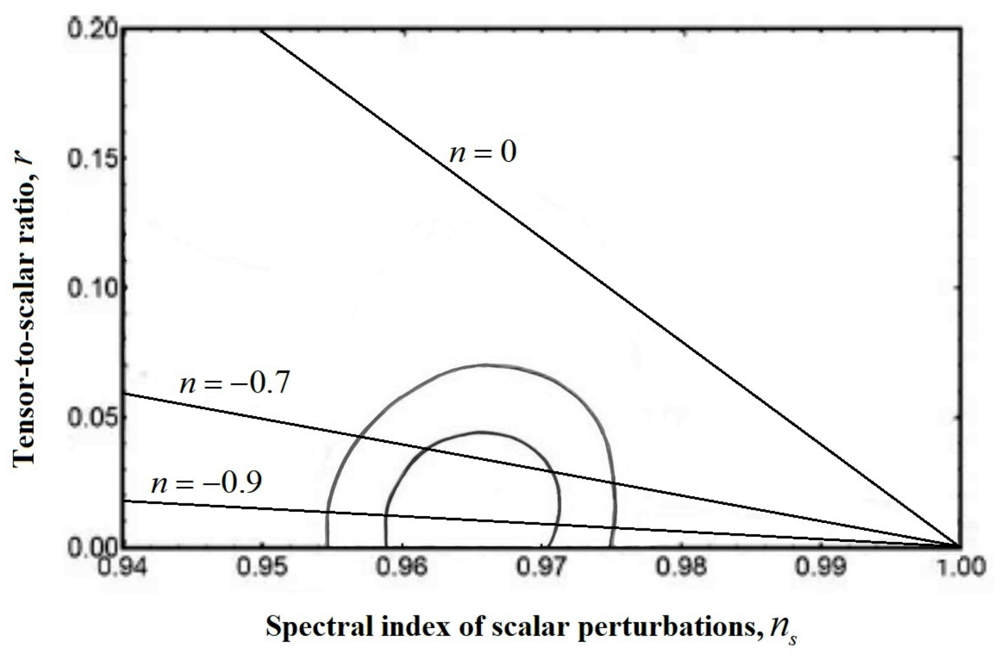
In Figure 1, the dependence (77) for the inflationary model with the Hubble parameter (57) is represented. As a criterion for verifying inflationary models according to observational constraints on the values of the parameters of cosmological perturbations, we will consider that the values of the tensor-to-scalar ratio r and the spectral index of scalar perturbations $n_S$ fall into the inner region corresponding to a 95% confidence level. Thus, Figure 1 demonstrates the previously obtained condition (79) for inflationary models under consideration.

Taking into account expression (60), we define the Hubble parameter and the first slow-roll parameter in terms of the e-fold number

$$H\left(N\right)=\lambda {\left(1+e^{2\beta N}\right)}^{1/2}{e}^{-\beta N},$$

(80)

$$ϵ=\beta {\left(1+e^{2\beta N}\right)}^{-1}.$$

(81)

From Equations (56) and (81), we have

$$\begin{array}{ccc}\hfill & & r=\frac{16(1+n)\beta }{1+e^{2\beta N}}.\hfill \end{array}$$

(82)

This function has a maximum for $2{\beta }_{0}N=1+W(1/e)$, where W is the Lambert function and $W(1/e)\simeq 0.28$. Thus, we have ${\beta }_0\simeq 0.64/N$, and for $N\simeq 60$, we obtain ${\beta }_0\simeq 0.01$.

This gives the maximal value for the tensor-to-scalar ratio

$$\begin{array}{ccc}\hfill & & r_{max}\simeq 0.038(1+n),\hfill \end{array}$$

(83)

and for $\left|n\right|\ll 1$, this is in agreement with constraint (40).

Nevertheless, after substituting $\beta \simeq 0.01$ and expression (83) with the condition $\left|n\right|\ll 1$ into (76), we obtain $n_S\simeq 1$, which does not correspond with constraint (39). Thus, conditions (79) on the constant parameter n are the correct ones for the verifiable hyperbolic inflationary model based on scalar-torsion gravity.

Moreover, from Equation (54) and conditions $N\simeq 60$ and $\beta \simeq {10}^{-2}$, we obtain the expression

$$\begin{array}{ccc}\hfill & & {\mathcal{P}}_S(N\simeq 60)=\frac{{\lambda }^{n+2}}{32{\pi }^2(n+1)\beta }{cosh}^2\left(\beta N\right)=2.1\times {10}^{-9},\hfill \end{array}$$

(84)

which gives the following restriction on the parameter ${10}^{-12}<\lambda <{10}^{-8}$ for $\delta =\beta \simeq {10}^{-2}$, and the non-minimal coupling constant $\xi =-\frac{n\beta }{4}\le 0.0025$ corresponding to weak coupling with a positive coupling constant.

Therefore, one can use constraints (79) and (84) on the constant parameters to analyze inflationary models with cosmological dynamics (59) for the other potential, the evolution of a scalar field and the type of scalar-torsion gravity, which can be obtained from generalized solutions (63)–(66) for the Hubble parameter $H=H\left(\varphi \right)$, differing from (68).

Thus, the inflationary models with the hyperbolic expansion law of the early universe can be verified by observational constraints on the values of the parameters of cosmological perturbations by taking into account the non-minimal coupling between the scalar field and torsion.

6.2. Inflation with Double-Well Potential

Now, we consider the inflationary model with the following Hubble parameter and scale factor [2,4,46]

$$H\left(t\right)=\lambda +\alpha exp(-\beta t),$$

(85)

$$\dot{H}=-\beta (H-\lambda ),$$

(86)

$$a\left(t\right)=a_{0}exp\left(\lambda t-\frac{\alpha }{\beta }{e}^{-\beta t}\right).$$

(87)

Moreover, we define the e-fold number for this model as follows

$$\begin{array}{ccc}\hfill & & N\left(t\right)=ln\left(\frac{a\left(t\right)}{a_0}\right)=\lambda t-\frac{\alpha }{\beta }{e}^{-\beta t},\hfill \end{array}$$

(88)

where its value at the beginning of inflation is $N(t=t_{beg})=0$, and at the end of the inflationary stage is $N(t=t_{end})\simeq 60$.

From expressions (52)–(53) and (85), we obtain the following slow-roll parameters for this inflationary model:

$$\begin{array}{ccc}\hfill & & ϵ=\frac{\alpha \beta e^{-\beta t}}{{(\lambda +\alpha e^{-\beta t})}^2},\delta =\frac{\beta }{2(\lambda +\alpha e^{-\beta t})},\hfill \end{array}$$

(89)

where slow-roll conditions $ϵ\ll 1$ and $\delta \ll 1$ are satisfied when $\beta \sim \lambda$ and $\alpha \gg \lambda$; moreover, the slow-roll parameters are decreasing functions.

The coupling function is

$$\begin{array}{ccc}\hfill & & F\left(t\right)={\left(1+\frac{\alpha }{\lambda }exp(-\beta t)\right)}^n,\hfill \end{array}$$

(90)

thus, condition (26) is satisfied for any value of the constant n.

Thus, at large times $t\to \infty$, one has $H=\lambda$ and $F=1$ from (57) and (62), and $\varphi =0$, $V=3{\lambda }^2$ and $\omega =1$ from (22) and (23), which correspond to the cases of the cosmological constant and TEGR.

Therefore, at large times, this cosmological model is reduced to the $\Lambda$CDM one for any model’s parameters.

6.2.1. Generalized Exact Solutions

From expressions (28)–(33), taking into account (85) and (86), the general solutions of dynamic equations for these models can be written as follows

$$V\left(\varphi \right)=\frac{H^n}{{\lambda }^n}\left[3H^2-\beta (n+1)(H-\lambda )\right],$$

(91)

$$\omega \left(\varphi \right)=\frac{2}{\beta }{\left(\frac{H}{\lambda }\right)}^n\left(\frac{n+1}{H-\lambda }\right){\left(\frac{dH}{d\varphi }\right)}^2,$$

(92)

$$F\left(\varphi \right)={\left(\frac{H\left(\varphi \right)}{\lambda }\right)}^n,$$

(93)

$$H\left(\varphi \right)=\lambda +\alpha exp(-\beta t),$$

(94)

where $H=H\left(\varphi \right)$ can be considered the generating function.

6.2.2. Special Class of Exact Solutions

For the Hubble parameter (85) from Equations (35)–(37), we obtain

$$\varphi \left(t\right)=\pm 2\sqrt{2\frac{\alpha }{\beta }}exp\left(-\frac{\beta }{2}t\right),$$

(95)

$$H\left(\varphi \right)=\lambda +\frac{\beta }{8}{\varphi }^2,$$

(96)

$$V\left(\varphi \right)=3{\lambda }^2{\left(1+\frac{\beta }{8\lambda }{\varphi }^2\right)}^{n+2}-\frac{{\beta }^2}{8}(n+1){\left(1+\frac{\beta }{8\lambda }{\varphi }^2\right)}^n{\varphi }^2,$$

(97)

$$F\left(\varphi \right)={\left(1+\frac{\beta }{8\lambda }{\varphi }^2\right)}^n,$$

(98)

$$\omega \left(\varphi \right)=(n+1){\left(1+\frac{\beta }{8\lambda }{\varphi }^2\right)}^n.$$

(99)

Under conditions $\frac{\beta }{8\lambda }{\varphi }^2\ll 1$ and $\beta \sim \lambda$, corresponding to the small field $\varphi \ll 1$ from (98), we obtain the non-minimal coupling at the first order

$$\begin{array}{ccc}\hfill & & F\left(\varphi \right)=1+\frac{n\beta }{8\lambda }{\varphi }^2+\mathcal{O}\left({\varphi }^4\right)\simeq 1-\xi {\varphi }^2,\hfill \end{array}$$

(100)

where $\xi =-\frac{n\beta }{8\lambda }$ is the coupling constant [39,40].

Moreover, under condition $\varphi \ll 1$ from (97), we obtain double-well potential [62,63]

$$\begin{array}{ccc}\hfill & & V\left(\varphi \right)\simeq A{\varphi }^4+B{\varphi }^2+3{\lambda }^2,\hfill \end{array}$$

(101)

where

$$A=\frac{{\beta }^2(n+1)}{64}\left[\frac{3}{2}(n+2)-\frac{\beta }{\lambda }n\right],$$

(102)

$$B=\frac{\beta }{8}\left[3\lambda (n+2)-\beta (n+1)\right].$$

(103)

For the partial case of minimal coupling $n=0$ from (95)–(99), we obtain the double-well potential as well:

$$\begin{array}{ccc}\hfill & & V\left(\varphi \right)=\frac{3{\beta }^2}{64}{\varphi }^4+\frac{\beta }{8}\left(6\lambda -\beta \right){\varphi }^2+3{\lambda }^2,\hfill \end{array}$$

(104)

with $F=1$, $\omega =1$, the same scalar field evolution $\varphi =\varphi \left(t\right)$, and the Hubble parameter $H=H\left(\varphi \right)$.

Both potentials, exact (97) and approximate (101), are reduced to (104) for $n=0$. Moreover, the difference between potentials (101) and (104) is defined by the values of the constant parameters, i.e., by the constant n.

Moreover, the spontaneous symmetry breaking in these inflationary models depend on the value of the constant n, namely, for the case $n=0$ for potential (104), this condition is $\beta >6\lambda$, and for potential (101), this condition is modified as $\beta >3\lambda \left(\frac{2+n}{1+n}\right)$.

As in the previous case, we will define the influence of the non-minimal coupling of a scalar field and torsion from observational constraints on the parameters of cosmological perturbations.

6.2.3. The Parameters of Cosmological Perturbations

To analyze the correspondence of this inflationary model to the observational constraints on the parameters of cosmological perturbations (38)–(40), we first consider the dependence tensor-to-scalar ratio from the spectral index of scalar perturbations.

From expression (89), for the case $\beta \sim \lambda$, we obtain

$$\begin{array}{ccc}\hfill & & ϵ=-4\frac{\lambda }{\beta }{\delta }^2+2\delta \simeq 2\delta .\hfill \end{array}$$

(105)

Thus, from expressions (55)–(56) and (105), we have

$$\begin{array}{ccc}\hfill & & r\simeq 16\left(\frac{1+n}{3-n}\right)(1-n_S).\hfill \end{array}$$

(106)

which restrict the possible values of the constant model’s parameter n due to the observational constraints.

The constant parameter n can be expressed in terms of the parameters of cosmological perturbations, as follows

$$\begin{array}{ccc}\hfill & & n=\frac{3r-16(1-n_S)}{r+16(1-n_S)},\hfill \end{array}$$

(107)

and after substituting observational constraints (39) and (40) into this expression, we obtain

$$\begin{array}{ccc}\hfill & & -1<n<-0.75.\hfill \end{array}$$

(108)

Thus, the inflationary models with double-well potential can be verified by observational constraints on the values of the parameters of cosmological perturbations by taking into account the non-minimal coupling between the scalar field and torsion with a power–law connection between the coupling function and the Hubble parameter (21), where constant parameter n is restricted by conditions (108).

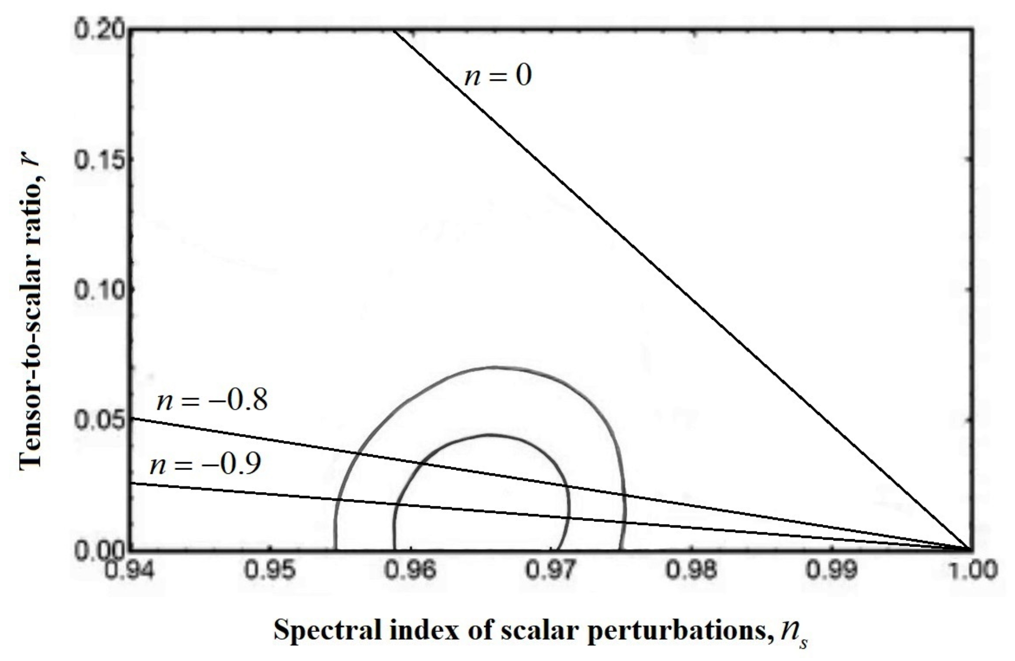
In Figure 2, the dependence (77) of the inflationary model with the Hubble parameter (85) demonstrates the previously obtained condition (108) for the inflationary model under consideration.

From the definition of the slow-roll parameter $ϵ=-\dot{H}/H^2$ for the Hubble parameter (85), we obtain

$$\begin{array}{ccc}\hfill & & ϵ=\frac{\beta (H-\lambda )}{H^2}.\hfill \end{array}$$

(109)

After substituting (109) into (54), and taking into account $\beta \sim \lambda$ and the quasi-de Sitter expansion of the early universe at the first inflationary stage $H\simeq \lambda +\alpha \simeq \alpha$, we obtain following condition on the constant parameters of the model

$$\begin{array}{ccc}\hfill & & {\mathcal{P}}_S=\frac{{\lambda }^n}{8{\pi }^2(n+1)\beta }\left(\frac{H^4}{H-\lambda }\right)\simeq \frac{{\alpha }^3{\lambda }^{n-1}}{8{\pi }^2(n+1)}\simeq 2.1\times {10}^{-9}.\hfill \end{array}$$

(110)

Moreover, for $\beta \sim \lambda$ and (108), we obtain $\xi \simeq 0.1$ in expression (100), which corresponds to a weak coupling with the positive coupling constant.

Finally, one can use constraints (108) and (110) on the constant parameters to analyze inflationary models with cosmological dynamics (87) for the other scalar-torsion gravity and parameters of cosmological models, which can be obtained from generalized solutions (91)–(94) for the Hubble parameter $H=H\left(\varphi \right)$, which differs from (96).

7. Conclusions

In this paper, we considered the influence of the non-minimal coupling of the scalar field and torsion in the models of cosmological inflation based on scalar-torsion theories of gravity compared to the teleparallel equivalent of general relativity.

To analyze the influence of non-minimal coupling, we considered a special case of a power–law relationship between the non-minimal coupling function and the Hubble parameter $F={\left(H/\lambda \right)}^n$, where the constant parameter n determines the specifics of this relationship and influences, the non-minimal coupling between the scalar field and torsion on the background parameters, and the parameters of cosmological perturbations.

As an example of this approach, we considered the models of cosmological inflation with hyperbolic cosine and double-well potentials based on TEGR and scalar-torsion gravity. The main motivation for considering these models was to fulfill condition (26), i.e., the transition of these cosmological models to the $\Lambda$CDM-models at large times. Thus, the effects of scalar-torsion modifications of the teleparallel equivalents of general relativity, in this case, are reduced to corrections to the potential and the values of the cosmological perturbation parameters.

Moreover, the generalized exact solutions (63)–(66) and (91)–(94) allow us to consider other types of scalar field potentials for these models. The restrictions on parameter n, which follow from the observational restrictions on the values of the parameters of cosmological perturbations, are also valid for generalized exact solutions.

For a special class of exact solutions, the influences of the non-minimal coupling of the field and torsion on the potential and values of the parameters of cosmological perturbations were estimated. Moreover, the reconstructed functions of non-minimal coupling (that determine the type of scalar-torsion of gravity for a small field) are reduced to non-minimal coupling.

Non-minimal coupling of the field and torsion affect the verification of these inflationary models by observational constraints. The procedure for verifying cosmological inflation models is reduced to estimating the constant parameters n and $\lambda$.

The estimates obtained for these parameters can be used in constructing other inflationary models with the considered cosmological dynamics based on other potential and types of scalar-torsion gravity following from the presented generalized solutions of the cosmological dynamics equations.

The prospect of developing the proposed approach involves its generalization in the case of $f\left(T\right)$-gravity with non-minimal coupling between the scalar field and torsion, which implies other ways of parameterizing the influence of non-minimal coupling on the nature of the implementation of the inflationary stage of the evolution of the early universe. Moreover, the development of the proposed approach involves the reconstruction of the spectra of relic gravitational waves in these inflationary models to assess the possibility of their registrations.