Article

Collaborative Production Task Decomposition and Allocation among Multiple Manufacturing Enterprises in a Big Data Environment

1
School of Informatics, Beijing Wuzi University, Beijing 101149, China
2
School of Economics and Management, Xidian University, Xi’an 710126, China
*
Author to whom correspondence should be addressed.
Symmetry 2021, 13(12), 2268; https://doi.org/10.3390/sym13122268
Submission received: 29 October 2021 / Revised: 17 November 2021 / Accepted: 18 November 2021 / Published: 28 November 2021
(This article belongs to the Special Issue Meta-Heuristics for Manufacturing Systems Optimization)

Abstract

:
To realize the efficient decomposition and allocation of collaborative production tasks and resources among multiple enterprises, a task decomposition and allocation model for collaborative production among multiple manufacturing enterprises is proposed in a big data environment. The model is designed for the efficient and fast processing of production information using big data technology. This study innovatively applies the 5S management method to conduct data preprocessing for a manufacturing service provider and design the operation process of data cleaning and conversion to improve the efficiency of data processing. A collaborative optimization model, based on a hierarchical model with seven levels and considering time, costs, and services, is established for the task of production to achieve a reasonable match between supply and demand. Finally, the correlation coefficients of manufacturing service providers are configured according to weight order, so that the weight order is symmetrical with that of the manufacturer. The model also engages all manufacturing service providers with different production capabilities in collaborative production. The model is proved to be scientific and effective by using a specific example. In cooperative production activities, the production tasks of small and medium-sized enterprises can be effectively allocated. It can also realize efficient cooperative production among multiple manufacturing enterprises.

1. Introduction

Currently, the strategic planning of schemes such as Industry 4.0 [1], Industrial Internet [2], and Made in China 2025 [3] creates opportunities for the digitalization of the manufacturing industry, solves the problem of information symmetry in the coordinated production of multiple enterprises, and presents advanced requirements for its development. The “one-stop” production model of traditional enterprises is no longer competitive, and the collaborative production model has become the “new favorite” of the manufacturing industry. In the collaborative production model, the decomposition and allocation of production tasks have become urgent issues for production and supplier services.
Task allocation is a key factor in the improvement of efficiency and reliability in the manufacturing system [4]. Scholars, both in China and overseas, have carried out relevant studies from various perspectives. Ebadifard [5] and Zhao et al. [6] studied the allocation of resources and tasks in specific situations. Liu et al. [7] and Zhou et al. [8] used public service platforms and crowdsourcing platforms as research objects, respectively, and discussed issues of production task allocation. Shahrabi et al. [9] and Erişgin et al. [10] studied the same dynamic job-shop scheduling on parallel machines, using fuzzy order parameter estimation with a receiving and dispatching optimal learning method.
In the process of studying task allocation, scholars often improve existing algorithms based on actual conditions, to find ways to improve workshop efficiency. For instance, Zhou et al. [11] studied the problem of the remote distributed collaborative development of complex products in a dynamic environment; in addition, they established a task allocation model of remote distributed multi-team collaborative development, based on an unconstrained coding method and a hybrid leapfrog algorithm. Chaouch et al. [12] proposed a hybrid ant colony algorithm combined with a local search to solve the distributed job shop scheduling problem. Kurdi et al. [13] used the new island-model genetic algorithm in the study of task assignment models. Nouri et al. [14] used a hybrid meta-heuristic algorithm to study the scheduling problem of machines and transportation robots regarding the task allocation problem. Salido et al. [15] used genetic algorithms to study energy efficiency issues in task allocation. Agárdi et al. [16] proposed a hybrid discrete bacterial memetic algorithm with simulated annealing, which is a major improvement in the research field of memetic algorithms.
The abovementioned scholars also focused on task allocation within a single enterprise or platform and have attained remarkable achievements, based on which, some scholars have tried to explore the allocation of cross-platform collaborative production tasks. For example, Zhou et al. [17] studied the decision-making of optimal product output when supply-chain members have different bargaining powers, regarding the collaborative production problem in the secondary supply chain, including upstream manufacturers and downstream treatment plants. Wang et al. [18] studied the complex collaborative production problem across various enterprises in a cloud-based manufacturing environment and proposed a hybrid set planning method to solve the scheduling problem of production resources. The above studies have achieved resource optimization among enterprises. However, there have been few studies on task decomposition and assignment integration among enterprises.
The application and promotion of 5G technology, cloud computing, the Internet of Things, and other novel technologies have accumulated a large amount of structured and unstructured data in the manufacturing industry worldwide. With the rapid expansion of the scale of the manufacturing industry and of the supply chain with its synergistic relationship, the contradiction between the production of massive amounts of data in the manufacturing industry and the lack of corresponding data-processing mechanisms is extremely prominent. Some scholars have conducted useful explorations of this problem. Meng et al. [19] solved the problem of traditional data center loads only pursuing resource utilization maximization by innovatively introducing a time utility function in the model construction and proposing an online heuristic dynamic resource allocation algorithm for data centers. Ren et al. [20] studied the information and knowledge interactions between subtasks in complex task scenarios. They proposed a mathematical model for the hybrid multi-objective task allocation optimization of the network. This was performed through the dynamic matching of task networks and service collaboration networks, comprehensively considering the competence and collaboration level of service groups. Zheng et al. [21] considered problems such as information interaction and distortion in collaborative production situations and proposed a task allocation method for multi-supplier collaborative production, based on big data. Wang et al. [22] proposed a task allocation algorithm for big data computing based on accurate user perception by using adaptive fuzzy clustering, topic extraction model, logistic regression, and other methods to solve the inefficient problem of the traditional random task allocation algorithm. Currently, relevant achievements focus on manufacturing-related data from various perspectives, such as information interaction granularity, interaction efficiency, and knowledge extraction. As the front-end input of the manufacturing task decomposition and distribution stage, the processing mechanisms of various techniques, such as rapid data acquisition, efficient data conversion, and accurate data analysis, need further study. Therefore, the 5s management method of data processing from the source can offer a good solution to issues with the efficiency of front-end input.
Studies have proved that having sufficient data mining and analysis is immensely beneficial to enterprises. The big data processing mechanism can improve the market competitiveness of the manufacturing industry by mining the hidden knowledge value and potential capabilities of industrial big data, assisting business leaders to form scientific and accurate decisions in various complex manufacturing environments [19]. Therefore, based on the characteristics of task decomposition and allocation for collaborative production, and the advantages of big data in data collection, processing, and analysis, the task allocation framework on the Hadoop platform is designed to build the task allocation model of multi-manufacturing enterprises to achieve cross-enterprise collaborative production in the shortest time and with the lowest cost.
Therefore, the contribution of this paper lies in the innovation and integration of 5S management methods, giving full play to the advantages of data mining in information interaction granularity, interaction efficiency and knowledge extraction. The efficiency of data acquisition and data conversion is improved effectively. This will contribute to the structural adjustment of traditional manufacturing industry and the rational allocation of production materials. It provides a new research perspective and theoretical basis for task decomposition and task integration among enterprises.

2. Conceptual Model of Task Decomposition and Allocation Based on Big Data

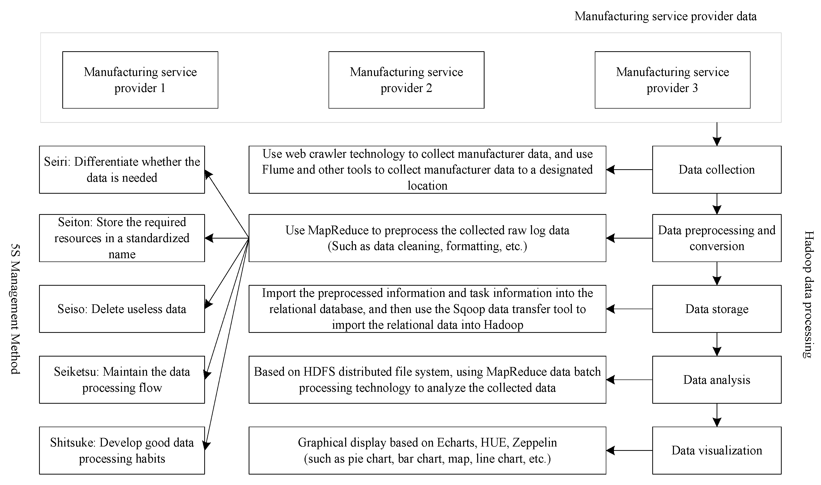
2.1. The 5S Management Method and Data Preprocessing

Data preprocessing using the 5S management method includes five elements. The first element is Seiri, which refers to the selection of the people and things involved by retaining the necessary ones and eliminating the rest. The data collection process may duplicate information for incomplete manufacturing service providers according to the data source, to determine its degree of importance. This includes the acquisition process of the repeated collection and merging of multiple sources of data, the retrieval error dataset, the data collection tools, and in the cause of completeness. All these operations can lead to errors, missing data, or redundancy in the dataset. Therefore, it is necessary to sort out the data, find all repeated or incomplete data through inspection and screening, and then remove them to ensure data accuracy in the database.
The second element is Seiton, which refers to placing the required resources in a fixed position. The data for the manufacturing service providers are named and stored in a fixed location. The operator can name the storage file. The following points must be noted: (1) data from different sources must be marked clearly; (2) multiple folders must be set up according to the complexity of task decomposition and distribution; and (3) these must be stored in a fixed location on the computer for ease of searching and use.
The third element is Seiso, which cleanses the workplace, deletes the original data that does not need to be collected in time, prevents invalid data association, and releases storage space.
The fourth element is Seiketsu, which is a continuation and extension of Seiri, Seiton, and Seiso. It refers to cleaning and tidying the database on the basis of the first three elements. It is a gradual and in-depth process, rather than a specific management link.
The final element is Shitsuke, which indicates that the cleaning process implements multiple steps of data cleaning, develops the practice of fully implementing the rules, and sticks to an appropriate routine.
Data cleaning is the process of repairing or deleting errors, damage, format errors, duplicates, or incomplete data in a data set. First, remove all unnecessary observations from the data set obtained by the crawler; second, identify outliers and check and filter them; third, perform a consistency check and deal with noise. The main process of data cleaning in this research is to write the Mapper part of the three common parts of the MapReduce program, Mapper, Reducer, and Job.
Since most of the data we encounter in real life is generally incomplete, it may lack attribute values or contain only aggregate data. Therefore, the integration of the 5S management method into the data-cleaning process can not only standardize the process but also remind researchers to pay attention to the standardization of their own operations. The above steps can reduce the amount of time and effort consumed by the process. Handling small details in an operation can remarkably improve the efficiency of data pretreatment and assist researchers in conducting scientific work more efficiently. A brief description of the 5S in the entire data-processing procedure is shown in Figure 1.

2.2. Conceptual Model of Manufacturing Task Decomposition and Allocation

To secure their position in a fiercely competitive market, it is essential for manufacturers to cooperate with regional and cross-regional multi-manufacturing enterprises for efficient production and mutual benefit. However, there are differences in production capacity, production efficiency, and service level among different manufacturing service providers. To cooperate to complete manufacturing tasks more efficiently, a conceptual model of task decomposition and allocation must be constructed.
Several manufacturing enterprises in collaborative production are required for a manufacturer to make full use of their resources, shorten product delivery time, and improve manufacturing efficiency. The information obtained regarding a particular product manufacturing process and production task is split according to the process flow. The production tasks are decomposed into various subtasks and then sent to the distribution unit, which shows the importance of cooperation between various production manufacturers. However, in this process, impracticable planning of the processing sequence and the assembly sequence will lead to cascade adjustment or the redistribution of manufacturing tasks, which will inevitably increase the costs of the cooperating manufacturing service providers. Therefore, to increase the utilization ratio of manufacturing resources and improve manufacturing efficiency, the subtasks must be accurately assigned to suitable suppliers, namely, according to the service standards of the manufacturer, distribution of the corresponding set of tasks, reduction of the rigid requirements for corporate capabilities, improvement of collaborative production between various manufacturing enterprises, and absorption of more small and medium-sized manufacturing service providers to join in collaborative production.
Inspired by the 5S management method and data processing, the conceptual model of task decomposition and allocation based on big data can be described as follows: customers release manufacturing demand information, such as product delivery time, quantity, and process requirements, and process massive quantities of data from manufacturing service providers through a 5S big data processing mechanism. The conceptual model can be divided into two processing methods, based on different data sources: (1) the internal data of the enterprise is imported directly to the Hadoop platform and transferred to the Hadoop distributed file system (HDFS) using the Flume tool to complete data storage; (2) the external data is obtained after data preprocessing (data cleaning) through a web crawler. Then, through data integration, data code and data transformation is stored in the Mysql database in higher quality datasets and passed on to the Hadoop platform via Sqoop tools. Similar to the internal data, the Flume tool is then used to transfer the information to the HDFS. For the processed external data and internal data, the MapReduce-based components Pig and Hive are used to analyze the data of manufacturing service providers, and ECharts and other tools are then used to analyze the results of the data visualization.
In collaborative production activities, it is beneficial to realize more efficient collaborative production among multiple manufacturing enterprises by assigning manufacturing tasks according to their production capacity levels. The manufacturing service provider information obtained by big data technology can be used as a reference for the evaluation criteria and scale-scoring of manufacturing service providers, laying a foundation for subsequent research on selecting the optimal manufacturing service provider, based on the analytic hierarchy process (AHP). The conceptual model of collaborative production task decomposition and allocation is shown in Figure 2.

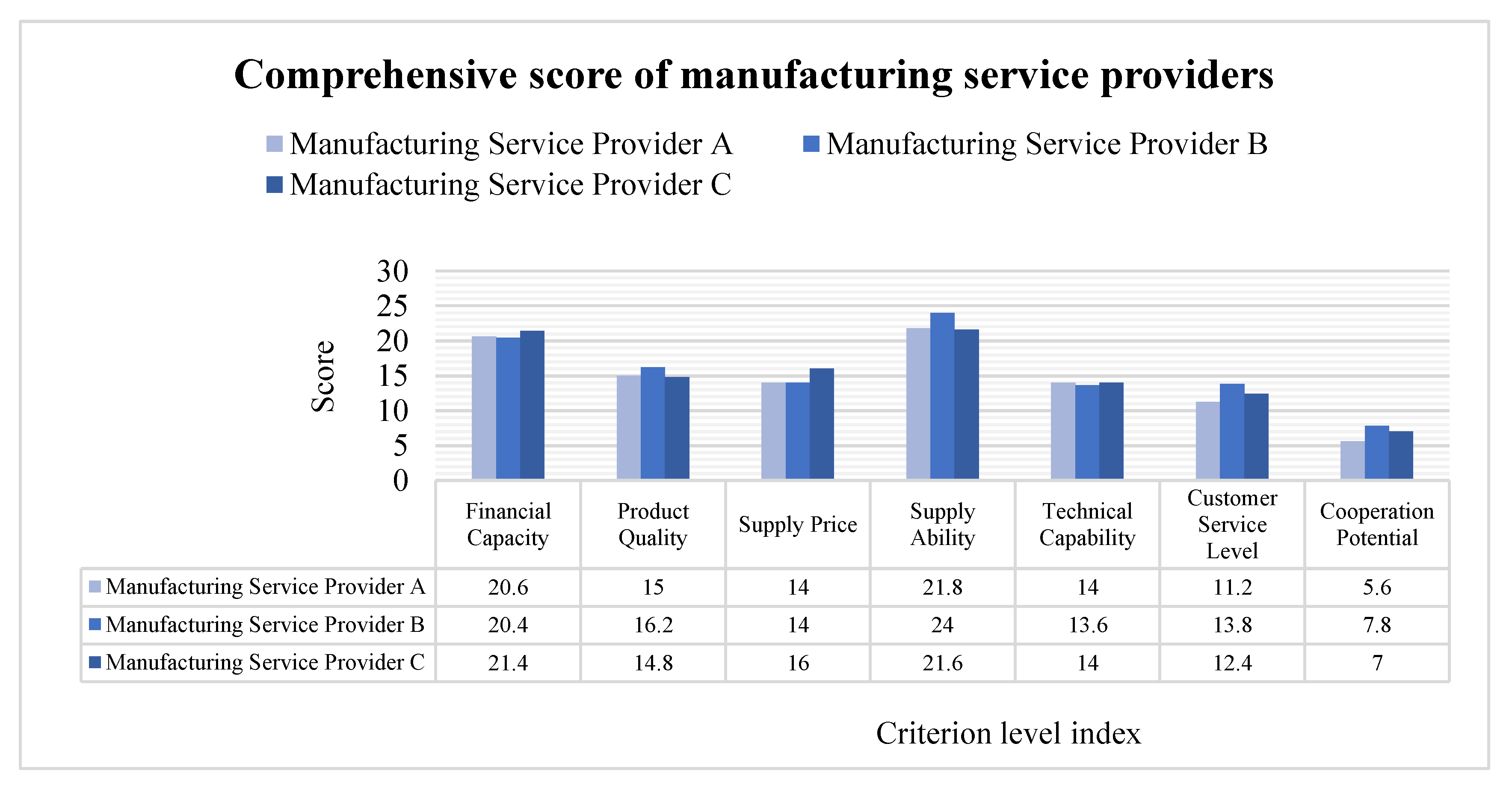
3. Selection of Manufacturing Service Providers

This section provides a precise description of the experimental results, their interpretation, and the experimental conclusions.
A big data processing mechanism is used to process the information from candidate manufacturing service providers, from which accurate and perfect data are obtained. Based on this, we invited technical experts from the industry, scientific research institutes, and technical workers of production lines to form expert groups for evaluation. The design of relevant indicators was summarized into a questionnaire, and each indicator was scored by combining online and offline methods. The scoring results were collected and summarized after removing the lowest and highest scores. Then, the average score of each indicator and the weight of each indicator were calculated through the AHP to obtain the evaluation results of each manufacturing service provider (see Appendix A for further details).
In his reading of both the domestic and foreign literature, G.W. Dickson [23] summarized the initial version of the evaluation indicator system in his earliest research in light of the consideration of the characteristics of collaboration between supplier production, manufacturing and service. In the process of selecting suppliers, it is necessary to pay attention to close integration and increase evaluation indicators, in line with their own needs and development status. Therefore, the supplier selection process must pay attention to manufacturing and services in relation to financial capacity, product quality, supply price, supply ability and technical capability, customer service level and cooperation potential. The supplier hierarchy model is shown in Figure 3.
In accordance with the AHP, the seven criterion-level indicators of the three candidate manufacturing suppliers are scored using the 1–9 scale method, and the judgment matrix is obtained by pairwise comparison. Hierarchical single ranking and consistency tests were conducted. Finally, the hierarchical total ranking composite weight table was obtained by a hierarchical total ranking and consistency test, as shown in Appendix A. Table A1 is the pairwise comparison matrix of criterion layer and target layer. The weight of each criterion to the target layer, multiplied by the weight of each indicator to the criterion layer (Table A2, Table A3, Table A4, Table A5, Table A6, Table A7 and Table A8) is the comprehensive weight value in Table A12. Table A9, Table A10 and Table A11 show the scores of the three manufacturing service providers. By scoring the three candidate manufacturing service providers and using a weighted comprehensive calculation, it can be seen that manufacturing service provider B has the highest score of 9.048, the second-highest is C with 8.594 points, and the lowest score is A with 8.239 points. To facilitate the subsequent calculation example analysis, the scores were normalized, and the final scores of A, B, and C were 0.318, 0.350, and 0.332, respectively. The weighted comprehensive scores of each index for the three manufacturing service providers are shown in Figure 4.
As shown in Figure 4, manufacturing service provider B offers the advantages of product quality, delivery capacity, customer service level, and cooperation potential. Manufacturing service provider C offers the obvious advantage of corporate financial strength, and manufacturing service providers A and C both offer the same technical advantages.

4. Mathematical Model of Task Decomposition and Assignment

4.1. Problem Description

For multiple manufacturing enterprises to conduct collaborative production, every enterprise seeks to maximize its economic benefits as the goal. The pursuit of economic efficiency maximization often leads to a drop in product quality and service levels; therefore, the collaborative manufacturing task decomposition and distribution solutions in the enterprise also need to ensure product quality and service level. Based on the data obtained from big data analysis, this model determines the values of the relevant parameters in the model and obtains specific decomposition and allocation methods for collaborative production tasks. The model aims to adjust the structure of the traditional manufacturing industry in the shortest time and within a reasonable budget, and realizes the rational allocation of resources.

4.2. Model Assumptions

In order to achieve the shortest time, reasonable cost and higher service evaluation, to achieve structural adjustment and reasonable allocation of resources, the following assumptions are made:
Hypothesis 1 (H1).
The weight values of the three manufacturing service providers will be used to allocate tasks scientifically and reasonably to improve efficiency because the optimal manufacturing service providers have been selected in the previous section and their weight ranking has been obtained.
Hypothesis 2 (H2).
The co-production task considers only the production of one part of the product.
Hypothesis 3 (H3).
The final assembly step of the product is performed by the manufacturing service provider responsible for the final collaborative production task. The total time required for the entire production task depends mainly on the mode of production. If the production task is linear, the total time is the sum of the time spent on the manufacturing and transportation of a single production task. If the production task is parallel production, the total time depends on the manufacturing service provider, which requires more processing time in the parallel production process. The cost required to complete the production task is composed of two parts: the cost generated by manufacturing and the cost generated by transportation.

4.3. Objective Function

The parameter variables to be listed for the model and their meanings are shown in Table 1, below.
The manufacturing service provider starts production after the production task is begun. The total manufacturing time, T, of the production task includes the manufacturing time, Tt, and the logistics and transportation time, Td, where Tdij is the time required by the product transportation process conducted by the manufacturing service provider, i. Therefore, the total manufacturing time, T, can be expressed as:
M i n T = T t + T d = ( i = 1 m j = 1 n T i j × N i j + i = 1 m j = 1 n T d i j ) × x i j
Production costs are a crucial factor in evaluating manufacturing service providers. The cost of collaborative production activities among multiple manufacturing enterprises is mainly composed of the manufacturing cost, Cm, and logistics cost, Cd. The manufacturing cost, Cdij, mainly includes the cost of purchasing raw materials, labor cost, raw material loss in the production process, and equipment maintenance cost. Logistics cost refers to the transportation cost generated in the process of product transportation, in which Cij refers to the cost generated in the process of product transportation, produced by the manufacturing service provider, i. The function of the production cost is:
M i n C = C m + C d = ( i = 1 m j = 1 n C i j × N i j + i = 1 m j = 1 n C d i j ) × x i j
Service quality is mainly reflected in the evaluation, which is relatively subjective. The indicators, as seen in Section 3, show that service quality is mainly reflected by service attitude, customer service response, problem-solving ability, and the effect of problem-solving. Let ω represent the weight coefficients of different manufacturing service providers, 0 ω i 1 and i = 1 q ω i = 1 .
Therefore, the objective function of service quality can be expressed as:
M a x S = ω S i j i = 1 m S i j
Normal production activities can be maintained only when the enterprise profits are positive. Therefore, when the enterprise income is greater than the cost, the production plan is feasible. The profit Q generated by production activities can be expressed as RC [24]. The cost of cooperative production among multiple manufacturing enterprises includes the production and cooperative costs of enterprises. The production cost of an enterprise mainly comes from factors such as purchasing raw materials, hiring employees, resource consumption, logistics cost, and equipment maintenance cost:
M a x Q = R C = N × P C = i = 1 m j = 1 n N i j × P i = 1 m j = 1 n N i j × C i j i = 1 m C d i j

4.4. Constraints

The constraints of collaborative production scheduling among multi-manufacturing enterprises include the start and end dates of orders, production capacity and undertaking capacity of specialized units, production quantity and working hours, production income and cost, the distance between enterprises, and service quality. The main constraints are as follows:
T T max
C C max
S min S
N × P i = 1 m j = 1 n N i j × C i j + i = 1 m C d i j
j = 1 n x i j = 1 , i = 1 , 2 , , m
Equation (5) indicates that the total time of actual collaborative production cannot exceed the delivery time required by the demander. Equation (6) requires that the actual cost of production should not be higher than the total maximum cost required by the manufacturing service provider. Equation (7) indicates that the quality of service provided in the service process cannot be less than the minimum quality of service required. Equation (8) indicates that normal production activities can be conducted only when the income is greater than the cost; otherwise, a collaborative production task cannot be established. Formula (9) restrains the collaborative task in collaborative production activities, and one collaborative task is assigned to only one manufacturer for production.

5. Test of the Mathematical Model of Task Decomposition and Assignment

Using the mobile phone manufacturing industry as an example, the key link in the manufacturing process of mobile phones is printed circuit boards (PCBs). The cooperative production task of a PCB assembly can be divided into: (1) task H1: PCB board loading; (2) task H2: printing machine to print solder paste; (3) task H3: SMT machine to paste electronic components; (4) task H4: reflux furnace welding; (5) task H5: semi-finished product test of the production task.
In this example, currently, 50 printed circuit boards need to be processed. After preliminary screening, there were three manufacturing service providers: P1, P2, and P3. The manufacturing service providers for each collaborative production task are selected from these three; that is, all three manufacturing service providers are capable of completing the above five production tasks. It can be seen that our goal is to successfully assign five collaborative production tasks to these candidate manufacturing service providers, and the five processing tasks in the task set {H1, H2, H3, H4, H5} will be completed according to number.
In Table 2, the second column lists the number of days required by the three manufacturing service providers to complete the five products, shown in days. The third column is the cost quoted by the three manufacturing service providers to complete the five products, taking the production price per square meter of low-end circuit boards of mobile phones as a reference, in yuan (CNY). Crawler is used to obtain the specific figures, and then the 5S management method is used to process the data and make reasonable assumptions.
Each time, the person ordering will score the performance of the manufacturing service provider during the process of providing services, with a scoring range of 0–1 to reflect a customer service level. When there are multiple historical evaluations, the score is the average of the historical evaluations. The data only affects the choice between the three manufacturing service providers and does not affect the validity of the research method. In Table 2, Table 3 and Table 4, since the actual situation is very random, with a variety of possible scenarios, values are randomly generated for analysis. The results are only used to draw the conclusions for this case study and have no influence on the whole study.
Table 2 shows the information table for manufacturing service providers participating in collaborative production tasks. Table 3 and Table 4 show the time and cost of transportation between the manufacturing service providers.
According to the information for each manufacturing service provider in Table 2, Table 3 and Table 4, the transportation cost and time between regions, and comprehensively considering the transportation cost and time consumption caused by the different locations of manufacturing service providers, the formula proposed above is used to solve the problem of optimal production resource allocation of the PCB manufacturing process in the mobile phone manufacturing industry.
In the example given in the calculation analysis, the first step is to determine the model of the indicators. Using the manufacturing process of a printed circuit board as an example, the number of customer orders is n = 100, and the product sales price is p = 1000, according to the agreement between the manufacturing service provider and the customer. Based on the data, it is calculated that the longest time spent in this case study is 44, and the minimum service quality is 3.05. As the data, in this case, is only used for calculation and analysis, there is no external demand from the demand side of the production service. For the convenience of calculation, we set T max to 44 and S min to 3.05. Similarly, according to the orders of magnitude of cost and profit in the case study, it is reasonable to assume that C max = 10,000 and Q max = 100,000 . This represents the weight coefficients of different manufacturing service providers in the objective function of the quality of service. In Section 3, the weight coefficients of three manufacturing service providers are normalized, and three different W values are obtained, with two decimal values reserved: ω 1 = 0.32 , ω 2 = 0.35 , and ω 3 = 0.33 .
In the initial parameter setting of the genetic algorithm, the population size was set as popsize = 120, the maximum number of iterations was set as maxGen = 50, the crossover probability, Pc = 0.8, and the mutation probability, Pm = 0.1. Finally, the optimal number of days is six, and the lowest cost is 3260 (Algorithms A1 and A2 show the solution of genetic algorithm for this case, see Appendix B for further details).
In general, genetic algorithms randomly generate individuals as the initial population. A co-production task, Hj, is co-produced by only one manufacturing service provider corresponding to chromosome xi; that is, co-production task H1 is co-produced by the manufacturing service provider corresponding to the serial number of the first chromosome x1. According to the three manufacturing service providers, the serial number of the initial set is numbered from 1 to 3, and the randomly generated initial population is shown in Figure 5.
Fitness is used to measure the performance of each individual in the population relatively accurately, and individuals with greater fitness are more likely to pass on their genes to the next generation. According to the research content, the service of the manufacturing service provider is taken as the optimization target. At the same time, the profit generated by limited production activities is the highest, and the decision variables, N, P, and Co. α1, α2 and α3, reflect the importance of profit, service level and time, respectively. If profit is more important and time efficiency is second, then α1 > α3 > α2. Considering the relationship between functions, the fitness function is defined as:
f ( i ) = α 1 Q i Q max + α 2 S i S max + α 3 T i T min
Selection depends on individual fitness values to calculate the probability of each individual’s genetic code appearing in the offspring, and the calculation randomly selects each individual to form the offspring population according to this probability. For example, we suppose that the number of individuals in each generation is M, and the fitness of each individual is fg. Then, the probability of g being selected is:
f g / g = 1 M f g
The research was carried out in a single-point crossing way. The individual gene code is in pairs, and a crossover location is generated with this opportunity. Two individuals can exchange their genetic code at the crossover location, thus forming two new offspring individuals. The principle of the crossover process is shown in Figure 6 and Figure 7. Mutations in genetic algorithms are achieved by changing a location on the chromosomes, or a location in their genes, as shown in Figure 8.
By referring to the work of Kucuksayacigil [25], research into genetic algorithm parameter fine-tuning can result in a high crossover rate and low mutation rate, and the solving effect is good. Therefore, the crossover rate and mutation rate are set as 0.8 and 0.05.
Variations in the genetic algorithm are accomplished by changing a certain position on the chromosome or genes at certain positions, as shown in Figure 8.
The termination condition selects the method by which the maximum iteration algebra is set. The flow chart of the specific calculation process of function-solving using the genetic algorithm is shown in Figure 9.
The calculation results show that the task H1 PCB board-loading is completed by P3. The task H2 printing machine is used to print solder paste to P3; the task H3 SMT electronic components are completed by P1; the task H4 reflux furnace welding is completed by P2; the task H5 semi-finished product test is completed by P2. Through the above arrangement, the PCB assembly process can be guaranteed to reach the optimal ratio of cooperative production via multiple manufacturing enterprises and to achieve a balance between the economic benefits and service quality of manufacturing enterprises.

6. Conclusions

Focusing on the three parts of big data processing, manufacturing service provider selection, and the task allocation model of collaborative production, the main research work and conclusions are as follows:
(1)
Big data technology was used to screen the information of candidate manufacturing service providers. The current popular big data platform, Hadoop processing technology, is used to screen candidate manufacturing service providers, and the 5S management method is integrated into the data processing. In addition, the specific process of data cleaning and conversion is established to improve the efficiency of data processing for manufacturing service providers.
(2)
Based on the understanding and analysis of the research results in related fields, AHP is selected to screen the optimal manufacturing service provider; the fuzzy evaluation indicators, due to the enterprise’s requirements or the difficulty of refining evaluation indicators, are quantified to render them more three-dimensional. One of the resulting three candidate manufacturing service providers is selected as the optimal service provider, according to the index weight ranking after normalization.
(3)
This paper builds a task allocation model that considers time, manufacturing cost, product quality, service quality, and other indicators, and refines the assumptions, parameter settings, objective functions, constraint conditions, and other issues of the task decomposition and allocation model for collaborative production among multiple manufacturing enterprises in the big data environment. Substituting specific data into the model solution proved the validity of the established model scheme.
(4)
A closed loop between big data technology and task allocation was completed. After data cleaning, the information from manufacturing service providers was integrated, and the AHP was used to quantify the indicators, which provided a new idea for the preparation of efficient collaborative production among multiple manufacturing enterprises. In terms of actual cooperative production activities among multi-manufacturing enterprises, production tasks are appropriately allocated to manufacturing service providers with different production capacities, to provide more opportunities for small- and medium-sized manufacturing enterprises to participate in the task of mass production.
At the same time, this study also has some limitations. The goal of this study is to achieve the goals of the shortest total time frame, lowest total cost and high overall service level in multi-enterprise cooperative production. As a result, the time frame and cost of an individual enterprise is rarely considered. In reality, due to the independence of each enterprise, because the task assigned is not a production plan that maximizes the firm’s profits, the individual firm is likely to withdraw from production. Therefore, in future studies, we can adopt additional constraints that consider the profits of individual firms. In the case of the lowest total cost, the method of offering some compensation to the enterprises that make “sacrifices” makes the research results more widely applicable.

Author Contributions

X.L. contributed to the writing of the first draft of this study, model building, case analysis, and analysis of relevant experimental results; F.L. contributed to the concept, method design, research work, and experimental analysis; Y.Y. contributed to the background research of this study and put forward constructive suggestions for revision. Y.X. and Y.Z. helped to analyze and make important suggestions for the framework of this article and to make some modifications to the original draft. All authors have read and agreed to the published version of the manuscript.

Funding

This study was supported by the National Social Science Fund of China, Research on the National Social Science Fund of China (20BJY185), Beijing Social Science Foundation(19ZDA12), Project of 2020 “Shipei plan” of Beijing Wuzi University, Beijing Collaborative Innovation Center for Intelligent Logistics System (BILSCI-2019KF-12), Jiangsu Key Laboratory of Transportation and Security (TTS2018-02), and Natural Science Foundation of Shaanxi Province (2021JM-146).

Institutional Review Board Statement

Not applicable.

Informed Consent Statement

Not applicable.

Data Availability Statement

Not applicable.

Conflicts of Interest

The authors declare no conflict of interest.

Appendix A

Table A1. Pairwise comparison matrix of criterion layer to target layer.
Select Manufacturing Service ProviderFinancial CapacityProduct QualitySupply PriceSupply AbilityTechnical CapabilityCustomer Service LevelCooperation Potential
Financial Capacity11/31/31/3152
Product Quality3113555
Supply Price3111/3554
Supply Ability31/331552
Technical Capability11/51/51/5111
Customer Service Level1/51/51/51/5111
Cooperation Potential1/21/51/41/2111
Sum82/713/4639/7192316
Table A2. Financial capacity index judgment matrix and weight value.
Financial CapacityHuman
Capital
Financial
Capital
Equity
Capital
Debt Paying
Ability
Ability to
Operate
ProfitabilityDevelopment
Capacity
Weight value
Human Capital11/311/31/41/51/30.0047
Financial Capital31311/21/31/30.108
Equity Capital11/311/31/31/31/50.046
Debt-Paying Ability3131111/30.140
Ability to Operate42311120.232
Profitability53511/21/21/20.182
Development Capacity33531/21/210.241
λmax = 7.421, CI = 0.07, RI = 1.36, CR = 0.05 < 1, Consistency test passed.
Table A3. Product quality index judgment matrix and weight value.
Product QualityQuality SystemQuality of Manufacturing Service ProviderManufacturing ProcessTest IndicatorsTraceabilityWeight Value
Quality System11/31/31/230.125
Quality of Manufacturing Service Provider311/21/230.205
Manufacturing Process321340.388
Test Indicators221/3120.208
Traceability1/31/31/41/210.073
λmax = 5.33, CI = 0.08, RI = 1.12, CR = 0.07 < 1, Consistency test passed.
Table A4. Supply price index judgment matrix and weight value.
Supply PricePrice LevelCost
Transparency
Payment
Period
Cost
Control
Weight Value
Price Level13220.406
Cost Transparency1/311/31/30.098
Payment Period1/23120.287
Cost Control1/231/210.208
λmax = 4.12, CI = 0.04, RI = 0.89, CR = 0.04 < 1, Consistency test passed.
Table A5. Supply ability index judgment matrix and weight value.
Supply AbilityProduction CapacityProduction ManagementProduction CapacityProduction ManagementSafety ManagementOrder FlexibilityWeight Value
Production Capacity1233230.310
Production Management1/211/221/220.130
Production Capacity1/32121/330.157
Production Management1/31/21/211/230.106
Safety Management1/2232130.230
Order Flexibility1/31/21/31/31/310.063
λmax = 6.36, CI = 0.07, RI = 1.26, CR = 0.05 < 1, Consistency test passed.
Table A6. Technical Capability index judgment matrix and weight value.
Technical CapabilityProduct DesignProduction TechnologyTechnological InnovationInnovation InvestmentWeight Value
Product Design12220.383
Production Technology1/21320.299
Technological Innovation1/21/311/20.125
Innovation Investment1/21/2210.190
λmax = 4.14, CI = 0.04, RI = 0.89, CR = 0.05 < 1, Consistency test passed.
Table A7. Customer service level index judgment matrix and weight value.
Customer Service LevelOrder
Confirmation
Service
Attitude
Customer Service ResponseProblem Handling EffectWeight Value
Order Confirmation12230.419
Service Attitude1/211/21/20.137
Customer Service Response1/2211/20.195
Problem-Handling Effect1/32210.248
λmax = 4.21, CI = 0.07, RI = 0.89, CR = 0.08 < 1, Consistency test passed.
Table A8. Cooperation potential index judgment matrix and weight value.
Cooperation PotentialBusiness RiskCooperation PotentialCompetitivenessWeight Value
Business Risk1330.588
Cooperation Potential1/311/20.159
Competitiveness1/3210.251
λmax = 3.05, CI = 0.02, RI = 0.52, CR = 0.05 < 1, Consistency test passed.
Table A9. Evaluation of manufacturing service provider A.
Manufacturing Service Provider AIndicatorsSynthesis Score
Financial CapacityHuman Capital2
Financial Capital2.6
Equity Capital3
Debt Paying Ability3
Ability to Operate3
Profitability3.6
Development Capacity3.4
Product QualityQuality System3.2
Quality of Manufacturing Service Provider3
Manufacturing Process2.8
Test Indicators3
Traceability3
Supply PricePrice Level4
Cost Transparency3
Payment Period3
Cost Control4
Supply AbilityProduction Capacity5
Production Management4
Production Capacity3.6
Production Management3
Safety Management3.2
Order Flexibility3
Technical CapabilityProduct Design3.8
Production Technology3
Technological Innovation3.2
Innovation Investment4
Customer Service LevelOrder Confirmation3
Service Attitude2
Customer Service Response3
Problem Handling Effect3.2
Cooperation PotentialBusiness Risk3
Cooperation Potential2.6
Competitiveness3
Table A10. Evaluation of manufacturing service provider B.
Manufacturing Service Provider BIndicatorsSynthesis Score
Financial CapacityHuman Capital3
Financial Capital2.6
Equity Capital3.2
Debt Paying Ability2.8
Ability to Operate3.2
Profitability2.6
Development Capacity3
Product QualityQuality System3.6
Quality of Manufacturing Service Provider3.4
Manufacturing Process3.2
Test Indicators2.8
Traceability3.2
Supply PricePrice Level4
Cost Transparency3
Payment Period4
Cost Control3
Supply AbilityProduction Capacity5
Production Management4
Production Capacity4
Production Management4
Safety Management4
Order Flexibility3
Technical CapabilityProduct Design3.2
Production Technology3
Technological Innovation3.4
Innovation Investment4
Customer Service LevelOrder Confirmation3.2
Service Attitude3.4
Customer Service Response3.8
Problem Handling Effect3.4
Cooperation PotentialBusiness Risk3.8
Cooperation Potential3.8
Competitiveness4
Table A11. Evaluation of manufacturing service provider C.
Manufacturing Service Provider CIndicatorsSynthesis Score
Financial CapacityHuman Capital3
Financial Capital3.2
Equity Capital3
Debt Paying Ability3
Ability to Operate3.4
Profitability2.8
Development Capacity3
Product QualityQuality System2.8
Quality of Manufacturing Service Provider3
Manufacturing Process3
Test Indicators3
Traceability3
Supply PricePrice Level5
Cost Transparency3
Payment Period4
Cost Control4
Supply AbilityProduction Capacity5
Production Management4
Production Capacity3
Production Management3.6
Safety Management3
Order Flexibility3
Technical CapabilityProduct Design3.8
Production Technology3
Technological Innovation3.2
Innovation Investment4
Customer Service LevelOrder Confirmation3
Service Attitude3.4
Customer Service Response3
Problem Handling Effect3
Cooperation PotentialBusiness Risk3
Cooperation Potential3.4
Competitiveness3.6
Table A12. Comprehensive score of three manufacturing service providers.
CriterionIndexComprehensive WeightOriginal RatingFinal Score
ABCABC
Financial CapacityHuman Capital0.0052330.0100.0150.015
Financial Capital0.0102.62.63.20.0260.0260.032
Equity Capital0.00433.230.0120.0130.012
Debt Paying Ability0.01432.830.0420.0390.042
Ability to Operate0.02333.23.40.0690.0740.078
Profitability0.0183.62.62.80.0650.0470.050
Development Capacity0.0233.4330.0780.0690.069
Product QualityQuality System0.0373.23.62.80.1180.1330.104
Quality of Manufacturing Service Provider0.06033.430.1800.2040.180
Manufacturing Process0.1122.83.230.3140.3580.336
Test Indicators0.06132.830.1830.1710.183
Traceability0.21533.230.6450.6880.645
Supply PricePrice Level0.0884450.3520.3520.440
Cost Transparency0.0213330.0630.0630.063
Payment Period0.0623440.1860.2480.248
Cost Control0.0454340.1800.1350.180
Supply AbilityProduction Capacity0.0735550.3650.3650.365
Production Management0.0314440.1240.1240.124
Production Capacity0.0373.6430.1330.1480.111
Production Management0.025343.60.0750.1000.090
Safety Management0.0543.2430.1730.2160.162
Order Flexibility0.0153330.0450.0450.045
Technical CapabilityProduct Design0.2053.83.23.80.7790.6560.779
Production Technology0.1603330.4800.4800.480
Technological Innovation0.0673.23.43.20.2140.2280.214
Innovation Investment 0.102440.4080.4080.408
Customer Service LevelOrder Confirmation0.18333.230.5490.5860.549
Service Attitude0.06023.43.40.1200.2040.204
Customer Service
Response
0.08533.830.2550.3230.255
Problem-Handling Effect0.1083.23.430.3460.3670.324
Cooperation PotentialBusiness Risk0.33133.830.9931.2580.993
Cooperation Potential0.0902.63.83.40.2340.3420.306
Competitiveness0.141343.60.4230.5640.508
Weight Sorting: B > C > A8.2399.0488.594

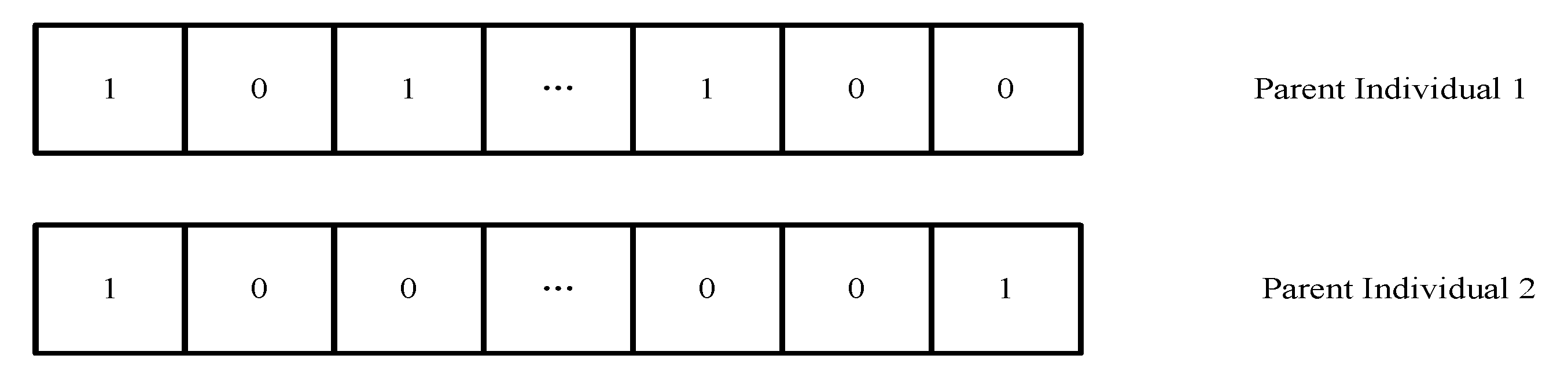
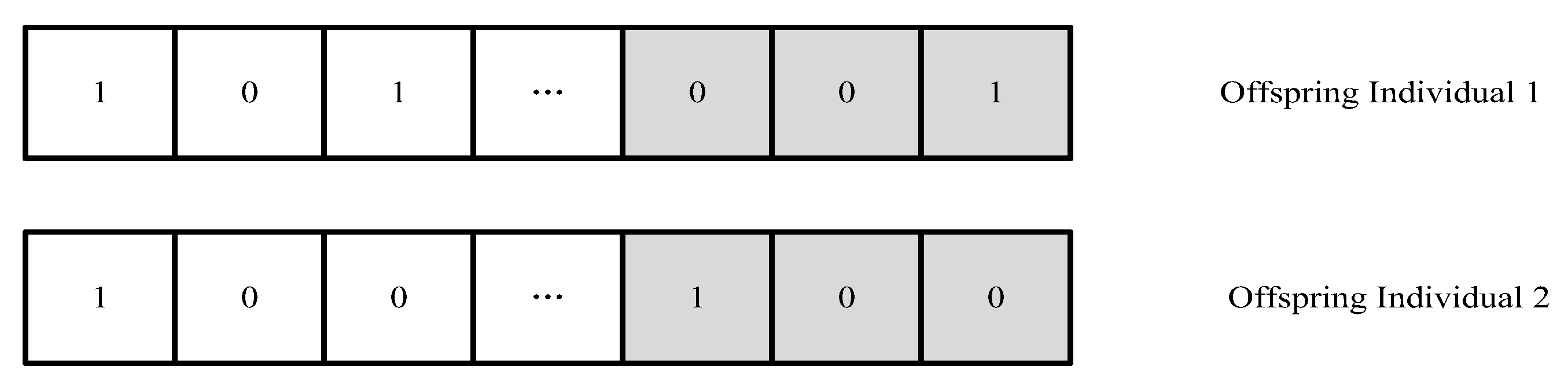
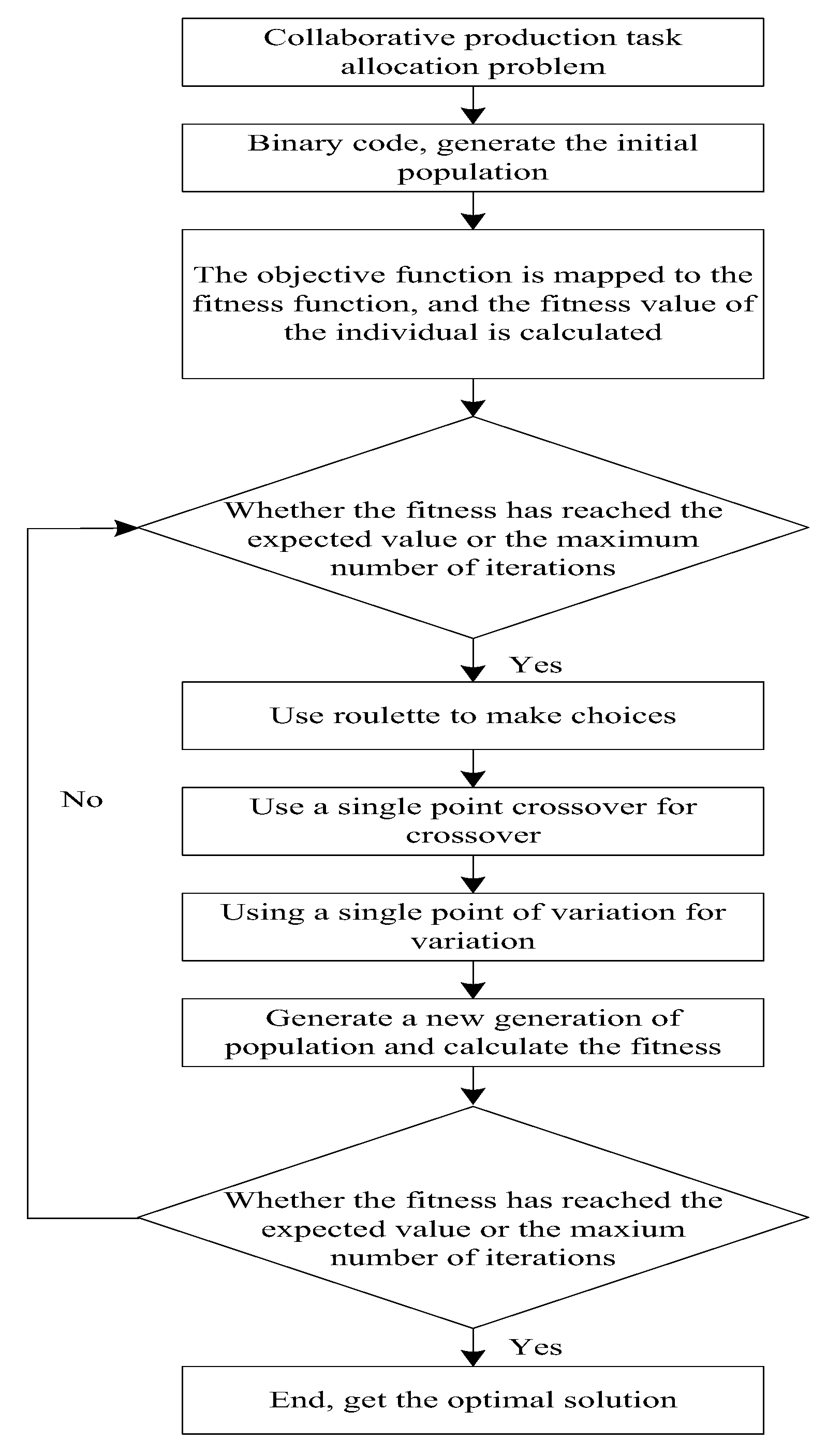
Appendix B. Genetic Algorithm

Algorithm A1. Pseudocode for GA
Input: instance Q,
size M of population,
rate Pc of crossover,
rate Pm of mutation,
number G of iterations,
value fmax of f(i)max
Output: solution Pop
//Initialization
    1 generate M feasible solutions randomly;
    2 save them in the population Pop;
//Loop until the terminal condition
    3 Initialize the empty population newPop
    4        Calculate the fitness f ( i ) = α 1 Q i Q max + α 2 S i S max + α 3 T i T min of each individual in population Pop
    5        Choose the best individuals according to the roulette system,
              g is chosen with probability f g / g = 1 M f g
    6        Two individuals were selected from population Pop by proportional selection algorithm based on fitness
    7        if (random (0,1) < Pc)
    8        Perform crossover operation on 2 individuals according to crossover probability Pc
    9        if (random (0, 1) < Pm)
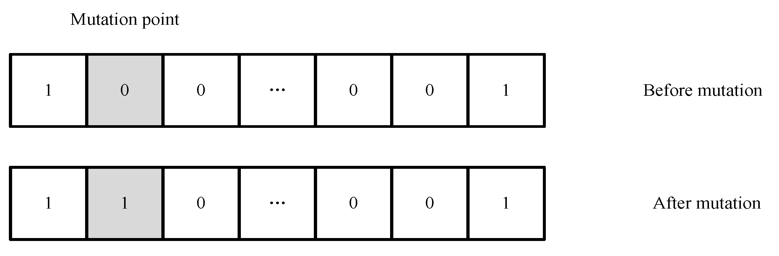
    10      Mutation operation was performed on 2 individuals according to mutation
probability Pm
    11 Add 2 new individuals to the population newPop
    12 until (M children are created)
    13 Replace Pop with newPop
    14 until (any chromosome score exceeds fmax, or reproductive algebra exceeds G)
Algorithm A2. Pseudocode for example of GA
1 Inherits the Problem superclass
2            Initialize name (function name, optionally set)
3            Set the row value of the matrix to i4 Set the column value of the matrix to j
5            Initialize Dim (Decision variable dimension
6            Initialize maxormins (list of target min Max flags, 1: minimize the target; -1: Maximize this goal)
7            Initialize varTypes (type of decision variable, 0: real; 1: integer)
8            Lower bound of decision variables
9            Upper bound of decision variables
10          Lower boundary of the decision variable (0 means the lower boundary of the variable is not included, 1 means included)
11          Upper boundary of a decision variable (0 means no upper boundary of the variable, 1 means included)
12          Call the parent class constructor to complete the instantiation
13          Defining the objective function
14          The decision variable matrix is obtained
15                        Returns the value of the matrix of service S
16                        Returns the value of the manufacturing time Tt matrix
17                        Returns the value of the transport time Td matrix
18                        Returns the value of the manufacturing cost Cm matrix
19                        Returns the value of the transport cost Cd matrix
20          The objective function1 is expressed
              as M i n T = T t + T d = ( i = 1 m j = 1 n T i j × N i j + i = 1 m j = 1 n T d i j ) × x i j
21          The objective function2 is expressed
              as M i n C = C m + C d = ( i = 1 m j = 1 n C i j × N i j + i = 1 m j = 1 n C d i j ) × x i j
22          The objective function3 is expressed
              as M a x Q = R C = N × P C = i = 1 m j = 1 n N i j × P i = 1 m j = 1 n N i j × C i j i = 1 m C d i j
23          The objective function4 is expressed
              as M a x S = ω S i j i = 1 m S i j , 0 ω i 1 and 0 ω i 1
24          Assign the obtained objective function value to ObjV of population pop

References

  1. Lu, Y. Industry 4.0: A survey on technologies, applications and open research issues. J. Ind. Inf. Integr. 2017, 6, 1–10. [Google Scholar] [CrossRef]
  2. Li, S.; Li, D.X.; Zhao, S. 5G Internet of Things: A survey. J. Ind. Inf. Integr. 2018, 10, 1–9. [Google Scholar] [CrossRef]
  3. Li, L. China’s manufacturing locus in 2025: With a comparison of “Made-in-China 2025” and “Industry 4.0”. Technol. Soc. Chang. 2018, 135, 66–74. [Google Scholar] [CrossRef]
  4. Cheng, Y.; Sun, F.Y.; Zhang, Y.P.; Tao, F. Task allocation in manufacturing: A review. J. Ind. Inf. Integr. 2019, 15, 207–218. [Google Scholar] [CrossRef]
  5. Ebadifard, F.; Babamir, S.M. Federated Geo-Distributed Clouds: Optimizing Resource Allocation Based on Request Type Using Autonomous and Multi-objective Resource Sharing Model. Big Data Res. 2021, 24, 100188. [Google Scholar] [CrossRef]
  6. Zhao, Y.; Guo, J.; Chen, X.; Hao, J.; Zheng, K. Coalition-based Task Assignment in Spatial Crowdsourcing. In Proceedings of the 2021 IEEE 37th International Conference on Data Engineering (ICDE), Chania, Greece, 1 April 2021; pp. 241–252. [Google Scholar]
  7. Liu, J.X.; Zhang, C. Research on member selection mechanism of virtual alliance and collaborative manufacturing among alliance enterprises under public service platform. Chin. J. Manag. Sci. 2020, 28, 126–135. [Google Scholar]
  8. Zhou, Q.; Fang, M. Research on crowdsourcing task allocation algorithm based on Multi-agent. Intell. Comput. Appl. 2019, 9, 104–107. [Google Scholar]
  9. Shahrabi, J.; Adibi, M.A.; Mahootchi, M. A reinforcement learning approach to parameter estimation in dynamic job shop scheduling. Comput. Ind. Eng. 2017, 110, 75–82. [Google Scholar] [CrossRef]
  10. Erişgin Barak, M.Z.; Koyuncu, M. Fuzzy Order Acceptance and Scheduling on Identical Parallel Machines. Symmetry 2021, 13, 1236. [Google Scholar] [CrossRef]
  11. Zhou, C.; Jiang, J.J.; Yin, M. Task allocation optimization for remote distributed collaborative development based on hybrid leapfrog algorithm. J. Ind. Eng. Eng. Manag. 2020, 34, 148–155. [Google Scholar]
  12. Chaouch, I.; Driss, O.B.; Ghedira, K. A novel dynamic assignment rule for the distributed job shop scheduling problem using a hybrid ant-based algorithm. Appl. Intell. 2019, 49, 1903–1924. [Google Scholar] [CrossRef]
  13. Kurdi, M. An effective new island model genetic algorithm for job shop scheduling problem. Comput. Oper. Res. 2016, 67, 132–142. [Google Scholar] [CrossRef]
  14. Nouri, H.E.; Driss, O.B.; Ghédira, K. Hybrid metaheuristics for scheduling of machines and transport robots in job shop environment. Appl. Intell. 2016, 45, 1–21. [Google Scholar] [CrossRef]
  15. Salido, M.A.; Escamilla, J.; Giret, A.; Barber, F. A genetic algorithm for energy-efficiency in job-shop scheduling. Int. J. Adv. Manuf. Technol. 2016, 85, 1303–1314. [Google Scholar] [CrossRef]
  16. Agárdi, A.; Nehéz, K.; Hornyák, O.; Koczy, L.T. A Hybrid Discrete Bacterial Memetic Algorithm with Simulated Annealing for Optimization of the Flow Shop Scheduling Problem. Symmetry 2021, 13, 1131. [Google Scholar] [CrossRef]
  17. Zhou, P.; Xu, H.; Lu, F. Manufacturer’s optimal output decision with bargaining power and co-production of by-products. Chin. J. Manag. Sci. 2020, 28, 156–163. [Google Scholar]
  18. Wang, X.L.; Chai, X.D.; Zhang, C.; Zhao, X.F. Cross-enterprise collaborative production scheduling algorithm in cloud manufacturing environment. Comput. Integr. Manuf. Syst. 2019, 25, 412–420. [Google Scholar]
  19. Meng, J.; Li, W.J.; Yu, G.R.; Wang, J.M.; Zhang, B.L. Utility maximization oriented dynamic resource allocation in data centers. Appl. Res. Comput. 2021, 38, 1728–1733, 1779. [Google Scholar]
  20. Ren, L.; Ren, M.L. Collaborative assignment model of intelligent manufacturing tasks based on mixed task networks. Comput. Integr. Manuf. Syst. 2018, 24, 838–850. [Google Scholar]
  21. Zheng, T.; Wang, Y.Y.; Xie, Z.H. Research on Multi-supplier collaborative Production Task allocation based on Big Data. Inn. Mong. Sci. Technol. Econ. 2019, 13, 44–47. [Google Scholar]
  22. Wang, Q.; Tan, L. Task assignment algorithm for big data group computing based on user topic accurate perception. J. Comput. Appl. 2016, 36, 2777–2783. [Google Scholar]
  23. Dickson, G.W. An analysis of vendor selection systems and decisions. J. Purch. 1966, 2, 5–17. [Google Scholar] [CrossRef]
  24. Al-Shihabi, S.; Al-Durgam, M. Multi-objective optimization for the multi-mode finance-based project scheduling problem. Front. Eng. Manag. 2020, 7, 223–237. [Google Scholar] [CrossRef]
  25. Kucuksayacigil, F.; Ulusoy, G. Hybrid genetic algorithm for bi-objective resource-constrained project scheduling. Front. Eng. Manag. 2020, 7, 426–446. [Google Scholar] [CrossRef]
Figure 1. The 5S management method and big data processing.
Symmetry 13 02268 g001
Figure 2. Conceptual model of task decomposition and allocation for collaborative production.
Symmetry 13 02268 g002
Figure 3. Manufacturing service provider hierarchy model.
Symmetry 13 02268 g003
Figure 4. Comprehensive scores of manufacturing service providers.
Symmetry 13 02268 g004
Figure 5. Initial population.
Symmetry 13 02268 g005
Figure 6. Parent individual binary code string.
Symmetry 13 02268 g006
Figure 7. Offspring individual binary code string.
Symmetry 13 02268 g007
Figure 8. Mutation operation.
Symmetry 13 02268 g008
Figure 9. Genetic algorithm-solving process.
Symmetry 13 02268 g009
Table 1. Symbols and their meanings.
VariableSignificance
RRevenue after a product is sold
CThe total cost of carrying out manufacturing activities in a manufacturing firm
QThe profit generated when i carries out production activities can be expressed by R-C
NThe number of products sold in a collaborative production activity
NijThe quantity produced by manufacturing service provider i to complete production task j
PThe price at which a product is sold in a collaborative production activity
iManufacturing service providers participating in collaborative production, i = 1,2,…,m
jCooperate with assigned tasks in production, j = 1,2,…,n
TThe total time it takes a manufacturing firm to complete manufacturing
xij1, Manufacturing service provider i is assigned to a collaborative production task j, and Nij exists
0, Manufacturing service provider i is not assigned to a collaborative production task j, Nij = 0
TtThe time generated during the transportation of the produced products, including the time required by Tij manufacturing service provider i to complete the production task j
TdThe time generated in the transportation process of the produced products, and the time generated in the transportation process of the product j produced by Tdij for manufacturing service provider i
CdThe cost generated in the process of product transportation, where Cdij is the time generated in the process of manufacturing service provider i producing product j
CmThe manufacturing cost generated during production or things, where Cij is the cost required by manufacturing service provider i to complete the production task j
SService evaluation of manufacturing service provider
SijService evaluation of manufacturing service provider i in completing production task j
Table 2. Information table of candidate manufacturing service providers participating in collaborative production tasks.
Production TaskTime/
Day
Cost (CNY)Service Quality EvaluationLocation of
Manufacturing
Service
Provider
Manufacturing Service
Provider
H122900.60AP1
2.52200.80BP2
32400.75CP3
H233200.90AP1
21700.70BP2
42500.80CP3
H378900.70AP1
79200.95BP2
68600.65CP3
H4156700.80AP1
125750.70BP2
145800.60CP3
H584000.50AP1
113200.90BP2
93000.80CP3
Table 3. Transport schedule between regions.
Transportation/DayRegion ARegion BRegion C
Region A023
Region B204
Region C340
Table 4. Transportation cost.
Cost (CNY)Region ARegion BRegion C
Region A0180260
Region B1800320
Region C2603200
Publisher’s Note: MDPI stays neutral with regard to jurisdictional claims in published maps and institutional affiliations.

