
A Novel Shuffled Frog-Leaping Algorithm for Unrelated Parallel Machine Scheduling with Deteriorating Maintenance and Setup Time

Abstract
:1. Introduction
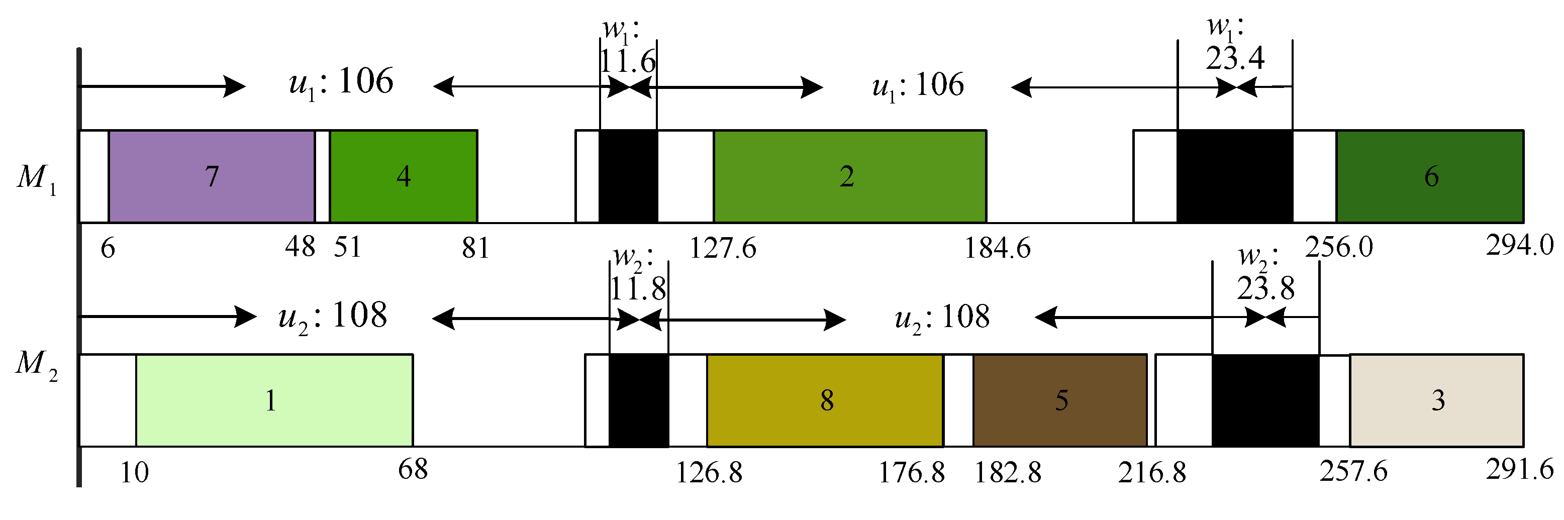
2. Problem Description
- ■
- Each job and machine is available at time zero.
- ■
- Each job can be processed on only one machine at a time.
- ■
- Operations cannot be interrupted.
- ■
- Preemption is not allowed.
3. Introduction to SFLA
4. DSFLA for UPMSP with Deteriorating PM and SDST
4.1. Initialization, Population Division, and the First Phase
4.2. The Second Phase
- (1)
- Perform population division, compute for all memeplexes, sort them in descending order of , and construct set .
- (2)
- For each memeplex , , repeat the following steps times if , execute global search between and a randomly chosen ; else perform global search between and a solution with for all .
- (3)
- For each memeplex ,
- 1
- sort all solutions in in the ascending order of makespan, suppose , and construct a set .
- 2
- Repeat the following steps times, and randomly choose a solution ; if , then select a solution by roulette selection based on , execute global search between and y, and update memory ; else execute global search between and a solution z with for all and update memory .
- (4)
- Execute multiple neighborhood searches on each solution .
- (5)
- Perform new population shuffling.
4.3. Algorithm Description
- (1)
- Initialization. Randomly produce initial population P with N solutions, and let initial be empty.
- (2)
- Population division. execute search process within each memeplex.
- (3)
- Perform population shuffling.
- (4)
- If the stopping condition of the first phase is not met, then go to step (2).
- (5)
- Execute the second phase until the stopping condition is met.
5. Computational Experiments
5.1. Instances and Comparative Algorithms
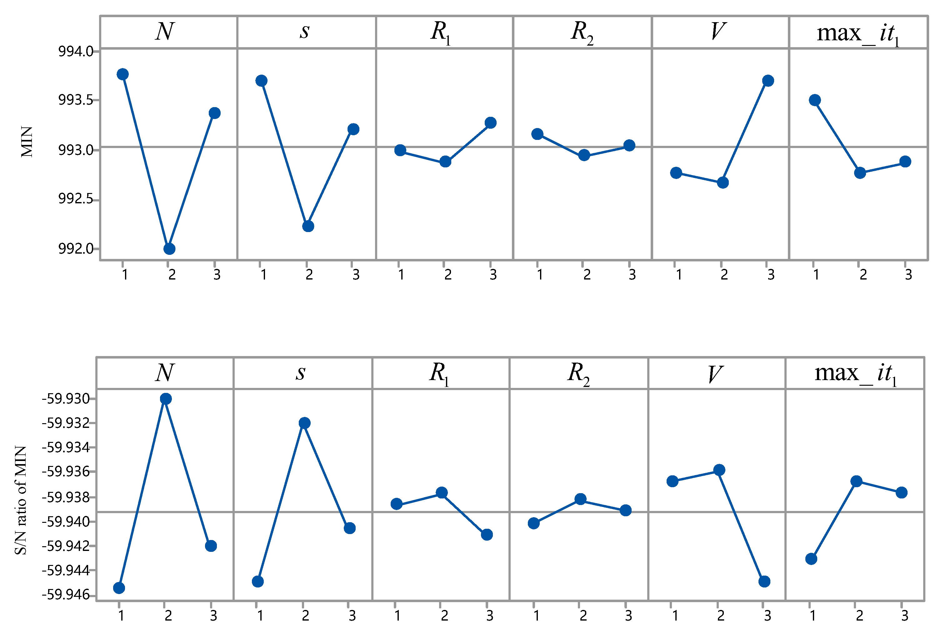
5.2. Parameter Settings
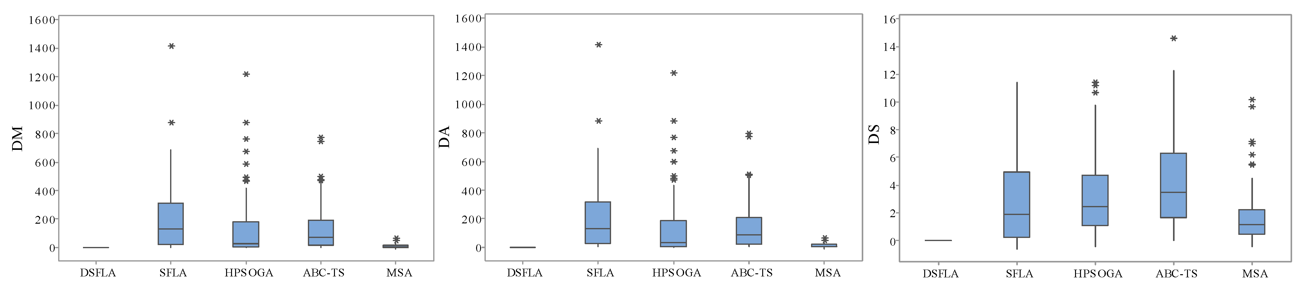
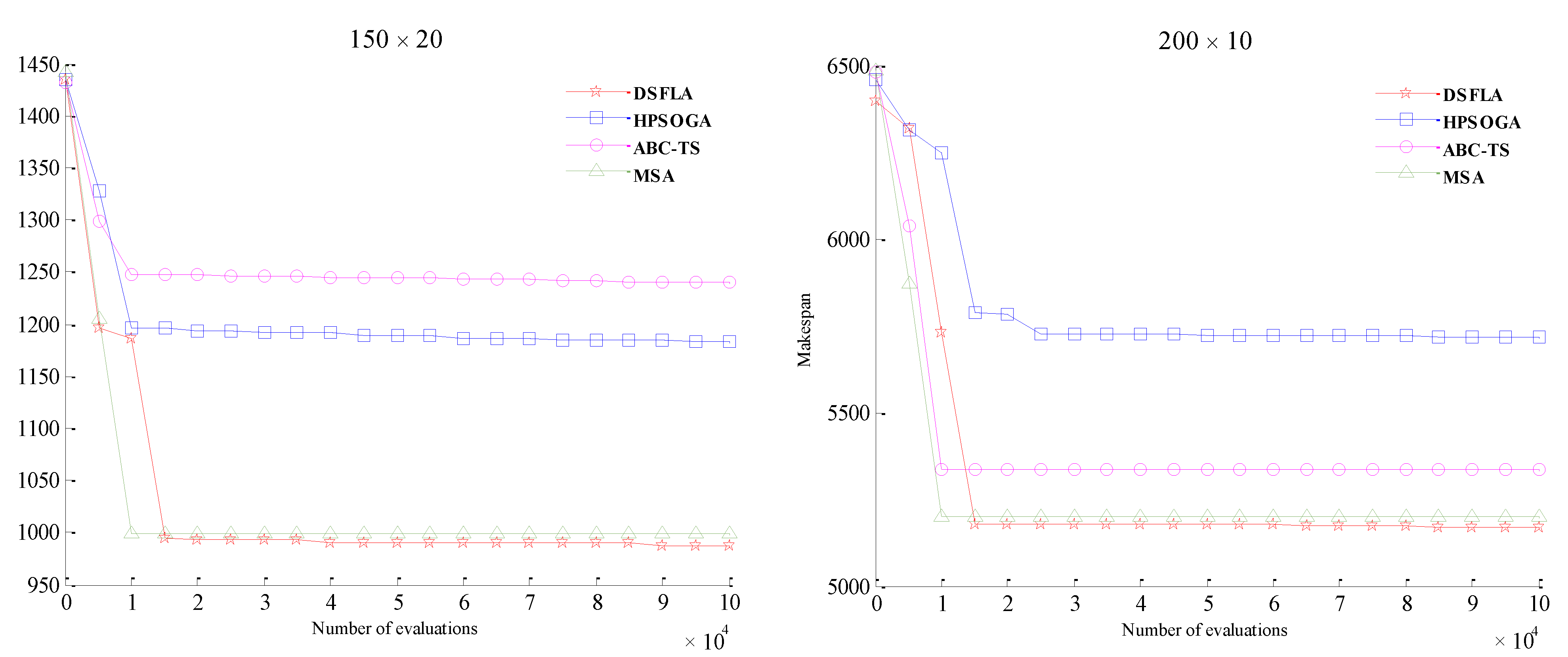
5.3. Results and Analyses
6. Conclusions
Author Contributions
Funding
Conflicts of Interest
References
- Kim, Y.-H.; Kim, R.-S. Insertion of new idle time for unrelated parallel machine scheduling with job splititing and machine breakdown. Comput. Ind. Eng. 2020, 147, 106630. [Google Scholar] [CrossRef]
- Wang, X.M.; Li, Z.T.; Chen, Q.X.; Mao, N. Meta-heuristics for unrelated parallel machines scheduling with random rework to minimize expected total weighted tardiness. Comput. Ind. Eng. 2020, 145, 106505. [Google Scholar] [CrossRef]
- Ding, J.; Shen, L.J.; Lu, Z.P.; Peng, B. Parallel machine scheduling with completion-time based criteria and sequence-dependent deterioration. Comput. Oper. Res. 2019, 103, 35–45. [Google Scholar] [CrossRef]
- Tavana, M.; Zarook, Y.; Santos-Arteaga, F.J. An integrated three-stage maintenance scheduling model for unrelated parallel machines with aging effect and multimaintenance activities. Comput. Ind. Eng. 2015, 83, 226–236. [Google Scholar] [CrossRef]
- Yang, D.L.; Cheng, T.C.E.; Yang, S.J.; Hsu, C.J. Unrelated parallel-machine scheduling with aging effects and multi-maintenance activities. Comput. Oper. Res. 2013, 39, 1458–1464. [Google Scholar] [CrossRef]
- Wang, S.J.; Liu, M. Multi-objective optimization of parallel machine scheduling integrated with multi-resources preventive maintenance planning. J. Manuf. Syst. 2015, 37, 182–192. [Google Scholar] [CrossRef]
- Gara-Ali, A.; Finke, G.; Espinouse, M.L. Parallel-machine scheduling with maintenance: Praising the assignment problem. Eur. J. Oper. Res. 2016, 252, 90–97. [Google Scholar] [CrossRef]
- Lei, D.M.; Liu, M.Y. An artificial bee colony with division for distributed unrelated parallel machine scheduling with preventive maintenance. Comput. Ind. Eng. 2020, 141, 106320. [Google Scholar] [CrossRef]
- Cheng, T.C.E.; Hsu, C.-J.; Yang, D.-L. Unrelated parallel-machine scheduling with deteriorating maintenance activities. Comput. Ind. Eng. 2011, 60, 602–605. [Google Scholar] [CrossRef]
- Hsu, C.-J.; Ji, M.; Guo, J.Y.; Yang, D.-L. Unrelated parallel-machine scheduling problems with aging effects and deteriorating maintenance activities. Infor. Sci. 2013, 253, 163–169. [Google Scholar] [CrossRef]
- Lu, S.J.; Liu, X.B.; Pei, J.; Thai, M.T.; Pardalos, P.M. A hybrid ABC-TS algorithm for the unrelated parallel-batching machines scheduling problem with deteriorating jobs and maintenance activity. Appl. Soft. Comput. 2018, 66, 168–182. [Google Scholar] [CrossRef]
- Allahverdi, A.; Gupta, J.N.; Aldowaisan, T. A review of scheduling research involving setup considerations. Omega 1999, 27, 219–239. [Google Scholar] [CrossRef]
- Parker, R.G.; Deana, R.H.; Holmes, R.A. On the use of a vehicle routing algorithm for the parallel processor problem with sequence dependent changeover costs. IIE Trans. 1977, 9, 155–160. [Google Scholar] [CrossRef]
- Kurz, M.; Askin, R. Heuristic scheduling of parallel machines with sequence-dependent set-up times. Int. J. Prod. Res. 2001, 39, 3747–3769. [Google Scholar] [CrossRef]
- Arnaout, J.P.; Rabad, G.; Musa, R. A two-stage ant colony optimization algorithm to minimize the makespan on unrelated parallel machines with sequence-dependent setup times. J. Intell. Manuf. 2010, 21, 693–701. [Google Scholar] [CrossRef]
- Vallada, E.; Ruiz, R. A genetic algorithm for the unrelated machine scheduling problem with sequence dependent setup times. Eur. J. Oper. Res. 2011, 211, 612–622. [Google Scholar] [CrossRef] [Green Version]
- Lin, S.W.; Ying, K.-C. ABC-based manufacturing scheduling for unrelated parallel machines with machine-dependent and job sequence-dependent setup times. Comput. Oper. Res. 2014, 51, 172–181. [Google Scholar] [CrossRef]
- Caniyilmaz, E.; Benli, B.; IIkay, M.S. An artificial bee colony algorithm approach for unrelated parallel machine scheduling with processing set restrictions, job sequence-dependent setup times, and due date. Int. J. Adv. Manuf. Technol. 2015, 77, 2105–2115. [Google Scholar] [CrossRef]
- Diana, R.O.M.; Filho, M.F.D.F.; Souza, S.R.D.; Vitor, J.F.D.A. An immune-inspired algorithm for an unrelated parallel machines scheduling problem with sequence and machine dependent setup-times for makespan minimisation. Neurocomputing 2015, 163, 94–105. [Google Scholar] [CrossRef]
- Wang, L.; Zheng, X.L. A hybrid estimation of distribution algorithm for unrelated parallel machine scheduling with sequence-dependent setup times. IEEE-CAA J. Autom. 2016, 3, 235–246. [Google Scholar]
- Ezugwu, A.E.; Akutsah, F. An improved firefly algorithm for the unrelated parallel machines scheduling problem with sequence-dependent setup times. IEEE Acc. 2018, 4, 54459–54478. [Google Scholar] [CrossRef]
- Fanjul-Peyro, L.; Ruiz, R.; Perea, F. Reformulations and an exact algorithm for unrelated parallel machine scheduling problems with setup times. Comput. Oper. Res. 2019, 10, 1173–1182. [Google Scholar] [CrossRef]
- Bektur, G.; Sarac, T. A mathematical model and heuristic algorithms for an unrelated parallel machine scheduling problem with sequence-dependent setup times, machine eligibility restrictions and a common server. Comput. Oper. Res. 2019, 103, 46–63. [Google Scholar] [CrossRef]
- Cota, L.P.; Coelho, V.N.; Guimaraes, F.G.; Souza, M.F. Bi-criteria formulation for green scheduling with unrelated parallel machines with sequence-depedent setup times. Int. Trans. Oper. Res. 2021, 28, 996–1007. [Google Scholar] [CrossRef]
- Avalos-Rosales, O.; Angel-Bello, F.; Alvarez, A.; Cardona-Valdes, Y. Including preventive maintenance activities in an unrelated parallel machine environment with dependent setup times. Comput. Ind. Eng. 2018, 123, 364–377. [Google Scholar] [CrossRef]
- Wang, M.; Pan, G.H. A novel imperialist competitive algoirthm with multi-elite individuals guidance for multi-objective unrelated parallel machine scheduling problem. IEEE Acc. 2019, 7, 121223–121235. [Google Scholar] [CrossRef]
- Eusuff, M.M.; Lansey, K.E.; Pasha, F. Shuffled frog-leaping algorithm: A memetic meta-heuristic for discrete optimization. Eng. Optim. 2006, 38, 129–154. [Google Scholar] [CrossRef]
- Rahimi-Vahed, A.; Mirzaei, A.H. Solving a bi-criteria permutation flow-shop problem using shuffled frog-leaping algorithm. Appl. Soft. Comput. 2008, 12, 435–452. [Google Scholar] [CrossRef]
- Pan, Q.K.; Wang, L.; Gao, L.; Li, J.Q. An effective shuffled frog-leaping algorithm for lot-streaming flow shop scheduling problem. Int. J. Adv. Manuf. Technol. 2011, 52, 699–713. [Google Scholar] [CrossRef]
- Li, J.Q.; Pan, Q.K.; Xie, S.X. An effective shuffled frog-leaping algorithm for multi-objective flexible job shop scheduling problems. Appl. Math. Comput. 2012, 218, 9353–9371. [Google Scholar] [CrossRef]
- Xu, Y.; Wang, L.; Liu, M.; Wang, S.Y. An effective shuffled frog-leaping algorithm for hybrid flow-shop scheduling with multiprocessor tasks. Int. J. Adv. Manuf. Technol. 2013, 68, 1529–1537. [Google Scholar] [CrossRef]
- Lei, D.M.; Guo, X.P. A shuffled frog-leaping algorithm for hybrid flow shop scheduling with two agents. Expert Syst. Appl. 2015, 42, 9333–9339. [Google Scholar] [CrossRef]
- Lei, D.M.; Guo, X.P. A shuffled frog-leaping algorithm for job shop scheduling with outsourcing options. Int. J. Prod. Res. 2016, 54, 4793–4804. [Google Scholar] [CrossRef]
- Lei, D.M.; Zheng, Y.L.; Guo, X.P. A shuffled frog-leaping algorithm for flexible job shop scheduling with the consideration of energy consumption. Int. J. Prod. Res. 2017, 55, 3126–3140. [Google Scholar] [CrossRef]
- Lei, D.M.; Wang, T. Solving distributed two-stage hybrid flowshop scheduling using a shuffled frog-leaping algorithm with memeplex grouping. Eng. Optim. 2020, 52, 1461–1474. [Google Scholar] [CrossRef]
- Cai, J.C.; Zhou, R.; Lei, D.M. Dynamic shuffled frog-leaping algorithm for distributed hybrid flow shop scheduling with multiprocessor tasks. Eng. Appl. Artif. Intell. 2020, 90, 103540. [Google Scholar] [CrossRef]
- Kong, M.; Liu, X.B.; Pei, J.; Pardalos, P.M.; Mladenovic, N. Parallel-batching scheduling with nonlinear processing times on a single and unrelated parallel machines. J. Glob. Optim. 2020, 78, 693–715. [Google Scholar] [CrossRef]
- Lu, K.; Ting, L.; Keming, W.; Hanbing, Z.; Makoto, T.; Bin, Y. An improved shuffled frog-leaping algorithm for flexible job shop scheduling problem. Algorithms 2015, 8, 19–31. [Google Scholar] [CrossRef] [Green Version]
- Fernez, G.S.; Krishnasamy, V.; Kuppusamy, S.; Ali, J.S.; Ali, Z.M.; El-Shahat, A.; Abdel Aleem, S.H. Optimal dynamic scheduling of electric vehicles in a parking lot using particle swarm optimization and shuffled frog leaping algorithm. Energies 2020, 13, 6384. [Google Scholar]
- Yang, W.; Ho, S.L.; Fu, W. A modified shuffled frog leaping algorithm for the topology optimization of electromagnet devices. Appl. Sci. 2020, 10, 6186. [Google Scholar] [CrossRef]
- Moayedi, H.; Bui, D.T.; Thi Ngo, P.T. Shuffled frog leaping algorithm and wind-driven optimization technique modified with multilayer perceptron. Appl. Sci. 2020, 10, 689. [Google Scholar] [CrossRef] [Green Version]
- Hsu, H.-P.; Chiang, T.-L. An improved shuffled frog-leaping algorithm for solving the dynamic and continuous berth allocation problem (DCBAP). Appl. Sci. 2019, 9, 4682. [Google Scholar] [CrossRef] [Green Version]
- Mora-Melia, D.; Iglesias-Rey, P.L.; Martínez-Solano, F.J.; Muñoz-Velasco, P. The efficiency of setting parameters in a modified shuffled frog leaping algorithm applied to optimizing water distribution networks. Water 2016, 8, 182. [Google Scholar] [CrossRef] [Green Version]
- Amiri, B.; Fathian, M.; Maroosi, A. Application of shuffled frog-leaping algorithm on clustering. Int. J. Adv. Manuf. Technol. 2009, 45, 199–209. [Google Scholar] [CrossRef]
- Elbeltagi, E.; Hegazy, T.; Grierson, D. A modified shuffled frog-leaping optimization algorithm: Applications to project management. Struct. Infrastruct. Eng. 2007, 3, 53–60. [Google Scholar] [CrossRef]
- Gao, J.Q.; He, G.X.; Wang, Y.S. A new parallel genetic algorithm for solving multiobjective scheduling problems subjected to special process constraint. Int. J. Adv. Manuf. Technol. 2009, 43, 151–160. [Google Scholar] [CrossRef]
- Afzalirad, M.; Rezaein, J. A realistic variant of bi-objective unrelated parallel machine scheduling problem NSGA-II and MOACO approaches. Appl. Soft Comput. 2017, 50, 109–123. [Google Scholar] [CrossRef]
- Mir, M.S.S.; Rezaeian, J. A robust hybrid approach based on particle swarm optimization and genetic algorithm to minimize the total machine load on unrelated parallel machines. Appl. Soft Comput. 2016, 41, 488–504. [Google Scholar]
- Taguchi, G. Introduction to Quality Engineering; Asian Productivity Organization: Tokyo, Japan, 1986. [Google Scholar]


| Job | 1 | 2 | 3 | 4 | 5 | 6 | 7 | 8 |
|---|---|---|---|---|---|---|---|---|
| 56 | 57 | 51 | 30 | 70 | 38 | 42 | 62 | |
| 58 | 55 | 34 | 69 | 34 | 57 | 69 | 50 |
| 1 | 2 | 3 | 4 | 5 | 6 | 7 | 8 | 1 | 2 | 3 | 4 | 5 | 6 | 7 | 8 | ||||
|---|---|---|---|---|---|---|---|---|---|---|---|---|---|---|---|---|---|---|---|
| 0 | 6 | 10 | 6 | 9 | 8 | 8 | 6 | 7 | j = 0 | 0 | 10 | 9 | 6 | 9 | 5 | 8 | 8 | 7 | |
| 1 | 8 | 0 | 10 | 5 | 7 | 10 | 8 | 10 | 7 | 1 | 5 | 0 | 7 | 9 | 9 | 7 | 9 | 8 | 6 |
| 2 | 8 | 5 | 0 | 6 | 7 | 9 | 8 | 5 | 8 | 2 | 8 | 7 | 0 | 8 | 10 | 6 | 7 | 7 | 5 |
| 3 | 7 | 7 | 9 | 0 | 7 | 5 | 9 | 9 | 7 | 3 | 10 | 6 | 7 | 0 | 6 | 10 | 8 | 5 | 5 |
| 4 | 5 | 7 | 7 | 10 | 0 | 6 | 10 | 6 | 9 | 4 | 6 | 10 | 9 | 5 | 0 | 7 | 9 | 10 | 7 |
| 5 | 8 | 10 | 6 | 7 | 10 | 0 | 9 | 6 | 5 | 5 | 10 | 7 | 10 | 9 | 9 | 0 | 8 | 6 | 6 |
| 6 | 8 | 7 | 7 | 9 | 8 | 6 | 0 | 8 | 10 | 6 | 6 | 6 | 10 | 7 | 7 | 6 | 0 | 5 | 8 |
| 7 | 6 | 9 | 8 | 9 | 3 | 9 | 7 | 0 | 10 | 7 | 6 | 7 | 9 | 5 | 8 | 8 | 6 | 0 | 8 |
| 8 | 8 | 10 | 10 | 5 | 7 | 5 | 5 | 6 | 0 | 8 | 10 | 9 | 8 | 6 | 7 | 6 | 7 | 9 | 0 |
| Parameters | Factor Level | ||
|---|---|---|---|
| 1 | 2 | 3 | |
| N | 60 | 80 | 100 |
| s | 4 | 5 | 10 |
| 30 | 50 | 70 | |
| 80 | 100 | 120 | |
| V | 220 | 240 | 260 |
| 5000 | 10,000 | 15,000 |
| Instance | DSFLA | SFLA | HPSOGA | ABC-TS | MSA | Instance | DSFLA | SFLA | HPSOGA | ABC-TS | MSA |
|---|---|---|---|---|---|---|---|---|---|---|---|
| 15 × 2 | 942 | 963 | 946 | 976 | 947 | 120 × 10 | 1889 | 2085 | 1908 | 2188 | 1889 |
| 15 × 4 | 365 | 368 | 379 | 381 | 375 | 120 × 15 | 1005 | 1151 | 1165 | 1403 | 1008 |
| 15 × 6 | 251 | 259 | 252 | 263 | 256 | 120 × 20 | 667 | 812 | 813 | 995 | 667 |
| 15 × 8 | 153 | 156 | 164 | 165 | 157 | 120 × 25 | 510 | 645 | 646 | 822 | 521 |
| 20 × 2 | 1343 | 1368 | 1340 | 1395 | 1404 | 120 × 30 | 391 | 519 | 516 | 677 | 388 |
| 20 × 4 | 500 | 509 | 504 | 514 | 514 | 150 × 10 | 2854 | 3097 | 2858 | 3543 | 2854 |
| 20 × 6 | 367 | 375 | 367 | 379 | 368 | 150 × 15 | 1413 | 1617 | 1614 | 1884 | 1413 |
| 20 × 8 | 258 | 260 | 260 | 267 | 258 | 150 × 20 | 985 | 1150 | 1166 | 1184 | 994 |
| 25 × 2 | 2031 | 2076 | 2076 | 2061 | 2078 | 150 × 25 | 673 | 825 | 810 | 1008 | 673 |
| 25 × 4 | 779 | 794 | 804 | 794 | 755 | 150 × 30 | 526 | 664 | 673 | 821 | 521 |
| 25 × 6 | 491 | 499 | 498 | 499 | 493 | 170 × 10 | 3650 | 3977 | 3650 | 4534 | 3654 |
| 25 × 8 | 365 | 367 | 365 | 376 | 368 | 170 × 15 | 1867 | 1881 | 1877 | 2422 | 1872 |
| 30 × 2 | 2730 | 2765 | 2796 | 2804 | 2736 | 170 × 20 | 1177 | 1358 | 1207 | 1613 | 1176 |
| 30 × 4 | 943 | 962 | 963 | 979 | 952 | 170 × 25 | 827 | 989 | 1010 | 1179 | 827 |
| 30 × 6 | 515 | 517 | 517 | 623 | 517 | 170 × 30 | 682 | 820 | 824 | 988 | 668 |
| 30 × 8 | 380 | 382 | 380 | 391 | 382 | 200 × 10 | 5171 | 5721 | 5176 | 5638 | 5179 |
| 35 × 2 | 3888 | 3978 | 3931 | 3945 | 3933 | 200 × 15 | 2480 | 2491 | 2513 | 2753 | 2485 |
| 35 × 4 | 1162 | 1164 | 1163 | 1175 | 1164 | 200 × 20 | 1418 | 1620 | 1636 | 1869 | 1419 |
| 35 × 6 | 645 | 653 | 650 | 665 | 657 | 200 × 25 | 1011 | 1196 | 1204 | 1389 | 1004 |
| 35 × 8 | 494 | 504 | 500 | 517 | 499 | 200 × 30 | 822 | 991 | 999 | 1168 | 829 |
| 50 × 10 | 514 | 524 | 523 | 667 | 516 | 220 × 10 | 6458 | 7046 | 7131 | 7936 | 6459 |
| 50 × 15 | 376 | 379 | 381 | 507 | 379 | 220 × 15 | 2853 | 3138 | 2856 | 3989 | 2865 |
| 50 × 20 | 260 | 268 | 273 | 368 | 260 | 220 × 20 | 1650 | 1894 | 1897 | 2443 | 1652 |
| 50 × 25 | 162 | 262 | 259 | 276 | 163 | 220 × 25 | 1184 | 1405 | 1600 | 1633 | 1202 |
| 50 × 30 | 159 | 160 | 170 | 271 | 160 | 220 × 30 | 994 | 1166 | 1191 | 1397 | 983 |
| 70 × 10 | 820 | 829 | 828 | 986 | 820 | 250 × 10 | 8908 | 9685 | 9784 | 9680 | 8916 |
| 70 × 15 | 511 | 520 | 519 | 658 | 514 | 250 × 15 | 3614 | 4020 | 4076 | 4079 | 3651 |
| 70 × 20 | 382 | 389 | 386 | 520 | 379 | 250 × 20 | 2175 | 2440 | 2488 | 2777 | 2177 |
| 70 × 25 | 267 | 375 | 276 | 395 | 269 | 250 × 25 | 1418 | 1841 | 1888 | 1891 | 1420 |
| 70 × 30 | 263 | 269 | 273 | 389 | 264 | 250 × 30 | 1189 | 1389 | 1422 | 1615 | 1173 |
| 100 × 10 | 1398 | 1566 | 1401 | 1647 | 1399 | 300 × 10 | 14,919 | 16,333 | 14,924 | 16,359 | 14,919 |
| 100 × 15 | 814 | 829 | 824 | 1004 | 819 | 300 × 15 | 5175 | 5726 | 6387 | 6241 | 5175 |
| 100 × 20 | 524 | 650 | 643 | 818 | 520 | 300 × 20 | 2859 | 3524 | 3615 | 3598 | 2861 |
| 100 × 25 | 390 | 513 | 502 | 652 | 393 | 300 × 25 | 1908 | 2484 | 2495 | 2503 | 1908 |
| 100 × 30 | 382 | 393 | 395 | 523 | 376 | 300 × 30 | 1420 | 1882 | 1909 | 2145 | 1422 |
| Instance | DSFLA | SFLA | HPSOGA | ABC-TS | MSA | Instance | DSFLA | SFLA | HPSOGA | ABC-TS | MSA |
|---|---|---|---|---|---|---|---|---|---|---|---|
| 15 × 2 | 942 | 963 | 946 | 976 | 947 | 120 × 10 | 1889 | 2098 | 1910 | 2198 | 1890 |
| 15 × 4 | 365 | 368 | 380 | 382 | 375 | 120 × 15 | 1005 | 1178 | 1168 | 1419 | 1008 |
| 15 × 6 | 251 | 260 | 254 | 267 | 256 | 120 × 20 | 669 | 819 | 818 | 1007 | 668 |
| 15 × 8 | 153 | 160 | 165 | 173 | 158 | 120 × 25 | 511 | 662 | 658 | 826 | 523 |
| 20 × 2 | 1343 | 1368 | 1342 | 1395 | 1404 | 120 × 30 | 393 | 523 | 522 | 681 | 389 |
| 20 × 4 | 500 | 509 | 506 | 517 | 514 | 150 × 10 | 2855 | 3103 | 2861 | 3569 | 2856 |
| 20 × 6 | 367 | 375 | 369 | 383 | 369 | 150 × 15 | 1413 | 1626 | 1624 | 1905 | 1414 |
| 20 × 8 | 258 | 261 | 262 | 268 | 258 | 150 × 20 | 993 | 1162 | 1168 | 1195 | 996 |
| 25 × 2 | 2031 | 2076 | 2076 | 2062 | 2078 | 150 × 25 | 673 | 831 | 818 | 1026 | 673 |
| 25 × 4 | 779 | 794 | 804 | 797 | 755 | 150 × 30 | 526 | 668 | 691 | 826 | 521 |
| 25 × 6 | 491 | 499 | 498 | 505 | 493 | 170 × 10 | 3653 | 3984 | 3650 | 4539 | 3655 |
| 25 × 8 | 365 | 367 | 365 | 381 | 368 | 170 × 15 | 1868 | 1896 | 1881 | 2433 | 1872 |
| 30 × 2 | 2730 | 2765 | 2796 | 2805 | 2736 | 170 × 20 | 1179 | 1372 | 1218 | 1619 | 1185 |
| 30 × 4 | 943 | 963 | 965 | 983 | 953 | 170 × 25 | 827 | 1001 | 1013 | 1191 | 828 |
| 30 × 6 | 515 | 518 | 518 | 625 | 518 | 170 × 30 | 684 | 825 | 837 | 1005 | 669 |
| 30 × 8 | 380 | 383 | 384 | 400 | 383 | 200 × 10 | 5172 | 5723 | 5177 | 5678 | 5179 |
| 35 × 2 | 3888 | 3978 | 3931 | 3946 | 3934 | 200 × 15 | 2480 | 2504 | 2520 | 2783 | 2485 |
| 35 × 4 | 1162 | 1164 | 1163 | 1177 | 1164 | 200 × 20 | 1421 | 1641 | 1644 | 1886 | 1420 |
| 35 × 6 | 646 | 654 | 651 | 667 | 658 | 200 × 25 | 1012 | 1202 | 1215 | 1401 | 1005 |
| 35 × 8 | 495 | 505 | 503 | 519 | 501 | 200 × 30 | 827 | 998 | 1007 | 1188 | 829 |
| 50 × 10 | 515 | 524 | 525 | 674 | 517 | 220 × 10 | 6459 | 7049 | 7133 | 7947 | 6459 |
| 50 × 15 | 377 | 379 | 384 | 515 | 380 | 220 × 15 | 2853 | 3141 | 2858 | 3995 | 2890 |
| 50 × 20 | 261 | 268 | 275 | 385 | 261 | 220 × 20 | 1650 | 1912 | 1919 | 2459 | 1653 |
| 50 × 25 | 163 | 262 | 264 | 280 | 165 | 220 × 25 | 1185 | 1410 | 1616 | 1645 | 1204 |
| 50 × 30 | 159 | 167 | 171 | 273 | 160 | 220 × 30 | 996 | 1176 | 1196 | 1410 | 984 |
| 70 × 10 | 821 | 829 | 831 | 1003 | 822 | 250 × 10 | 8909 | 9691 | 9788 | 9701 | 8918 |
| 70 × 15 | 512 | 520 | 521 | 667 | 515 | 250 × 15 | 3615 | 4029 | 4084 | 4087 | 3651 |
| 70 × 20 | 382 | 389 | 391 | 524 | 380 | 250 × 20 | 2177 | 2471 | 2498 | 2784 | 2177 |
| 70 × 25 | 268 | 375 | 278 | 396 | 270 | 250 × 25 | 1419 | 1855 | 1899 | 1906 | 1421 |
| 70 × 30 | 263 | 269 | 276 | 392 | 267 | 250 × 30 | 1190 | 1404 | 1429 | 1621 | 1173 |
| 100 × 10 | 1400 | 1566 | 1403 | 1652 | 1400 | 300 × 10 | 14,921 | 16,335 | 14,927 | 16,364 | 14,920 |
| 100 × 15 | 815 | 829 | 827 | 1019 | 823 | 300 × 15 | 5176 | 5734 | 6388 | 6269 | 5175 |
| 100 × 20 | 526 | 650 | 651 | 825 | 521 | 300 × 20 | 2860 | 3546 | 3618 | 3627 | 2862 |
| 100 × 25 | 390 | 513 | 513 | 667 | 394 | 300 × 25 | 1909 | 2502 | 2502 | 2508 | 1909 |
| 100 × 30 | 384 | 393 | 397 | 529 | 378 | 300 × 30 | 1421 | 1897 | 1916 | 2165 | 1423 |
| Instance | DSFLA | SFLA | HPSOGA | ABC-TS | MSA | Instance | DSFLA | SFLA | HPSOGA | ABC-TS | MSA |
|---|---|---|---|---|---|---|---|---|---|---|---|
| 15 × 2 | 0.00 | 0.00 | 0.00 | 0.00 | 0.60 | 120 × 10 | 0.00 | 8.72 | 1.20 | 10.06 | 0.75 |
| 15 × 4 | 0.00 | 0.00 | 0.90 | 0.46 | 0.66 | 120 × 15 | 1.50 | 9.40 | 2.84 | 5.83 | 0.00 |
| 15 × 6 | 0.65 | 1.20 | 1.77 | 2.22 | 0.30 | 120 × 20 | 0.87 | 3.50 | 5.10 | 5.85 | 0.66 |
| 15 × 8 | 1.50 | 2.21 | 1.04 | 2.30 | 1.57 | 120 × 25 | 0.66 | 5.83 | 11.31 | 2.75 | 1.64 |
| 20 × 2 | 0.00 | 0.00 | 2.10 | 0.00 | 0.46 | 120 × 30 | 1.47 | 2.21 | 5.76 | 3.10 | 0.94 |
| 20 × 4 | 0.00 | 0.00 | 2.29 | 2.32 | 0.49 | 150 × 10 | 1.25 | 3.69 | 4.27 | 9.70 | 1.86 |
| 20 × 6 | 0.00 | 0.43 | 1.73 | 1.61 | 1.75 | 150 × 15 | 0.80 | 7.45 | 10.06 | 11.95 | 0.54 |
| 20 × 8 | 0.64 | 0.60 | 2.28 | 0.83 | 0.54 | 150 × 20 | 2.80 | 5.70 | 2.49 | 5.55 | 1.18 |
| 25 × 2 | 0.00 | 0.00 | 0.00 | 0.80 | 1.20 | 150 × 25 | 0.00 | 3.24 | 3.75 | 7.00 | 1.31 |
| 25 × 4 | 0.00 | 0.00 | 0.00 | 1.04 | 0.00 | 150 × 30 | 0.00 | 2.46 | 7.35 | 3.10 | 0.30 |
| 25 × 6 | 0.40 | 0.00 | 0.30 | 2.92 | 0.00 | 170 × 10 | 0.98 | 5.54 | 2.02 | 2.76 | 2.19 |
| 25 × 8 | 0.00 | 0.30 | 0.00 | 2.27 | 0.40 | 170 × 15 | 0.49 | 8.59 | 4.23 | 6.99 | 0.00 |
| 30 × 2 | 0.00 | 0.00 | 0.00 | 0.40 | 0.00 | 170 × 20 | 0.60 | 5.84 | 10.41 | 5.12 | 2.97 |
| 30 × 4 | 0.00 | 0.92 | 2.40 | 1.60 | 1.36 | 170 × 25 | 1.20 | 5.24 | 3.67 | 4.68 | 1.72 |
| 30 × 6 | 0.00 | 0.66 | 1.03 | 1.20 | 1.09 | 170 × 30 | 1.86 | 3.87 | 11.79 | 6.68 | 0.64 |
| 30 × 8 | 0.63 | 0.93 | 3.78 | 4.61 | 1.81 | 200 × 10 | 1.10 | 1.26 | 1.15 | 13.37 | 3.25 |
| 35 × 2 | 0.00 | 0.00 | 0.00 | 0.49 | 0.64 | 200 × 15 | 0.30 | 9.48 | 5.87 | 10.91 | 0.30 |
| 35 × 4 | 0.00 | 0.30 | 0.00 | 3.15 | 0.60 | 200 × 20 | 1.99 | 10.41 | 6.59 | 5.95 | 1.36 |
| 35 × 6 | 1.18 | 0.84 | 0.23 | 1.43 | 0.30 | 200 × 25 | 0.30 | 3.81 | 8.62 | 6.43 | 0.50 |
| 35 × 8 | 0.77 | 0.91 | 3.22 | 1.75 | 1.94 | 200 × 30 | 3.33 | 5.29 | 5.41 | 7.42 | 0.78 |
| 50 × 10 | 0.49 | 2.68 | 1.94 | 3.68 | 0.80 | 220 × 10 | 0.40 | 1.75 | 1.84 | 6.78 | 0.30 |
| 50 × 15 | 0.40 | 1.52 | 3.03 | 4.76 | 0.87 | 220 × 15 | 1.02 | 2.96 | 3.16 | 3.11 | 11.20 |
| 50 × 20 | 0.15 | 1.65 | 2.19 | 5.80 | 0.38 | 220 × 20 | 0.30 | 8.56 | 8.77 | 11.27 | 3.04 |
| 50 × 25 | 2.70 | 1.64 | 5.19 | 2.26 | 1.89 | 220 × 25 | 1.94 | 3.22 | 7.75 | 5.72 | 2.69 |
| 50 × 30 | 0.00 | 1.62 | 1.16 | 1.71 | 0.49 | 220 × 30 | 0.48 | 5.39 | 5.05 | 6.95 | 0.98 |
| 70 × 10 | 1.02 | 3.75 | 1.11 | 9.89 | 2.12 | 250 × 10 | 1.19 | 3.81 | 4.67 | 7.66 | 0.81 |
| 70 × 15 | 1.10 | 2.56 | 2.94 | 4.61 | 1.76 | 250 × 15 | 0.46 | 4.72 | 5.90 | 4.36 | 0.00 |
| 70 × 20 | 0.49 | 1.92 | 4.85 | 2.87 | 1.30 | 250 × 20 | 1.08 | 13.19 | 8.65 | 4.07 | 0.90 |
| 70 × 25 | 2.77 | 2.03 | 1.01 | 1.76 | 0.89 | 250 × 25 | 2.10 | 7.69 | 9.60 | 9.52 | 1.76 |
| 70 × 30 | 0.65 | 2.00 | 2.46 | 2.09 | 1.36 | 250 × 30 | 0.49 | 6.70 | 8.72 | 7.08 | 0.49 |
| 100 × 10 | 1.85 | 5.68 | 1.20 | 2.17 | 0.54 | 300 × 10 | 1.37 | 2.27 | 3.41 | 4.04 | 0.66 |
| 100 × 15 | 1.50 | 1.90 | 2.70 | 5.06 | 3.36 | 300 × 15 | 0.46 | 5.14 | 3.67 | 9.68 | 0.30 |
| 100 × 20 | 1.30 | 2.83 | 5.44 | 4.52 | 1.25 | 300 × 20 | 1.56 | 8.65 | 2.39 | 14.59 | 1.81 |
| 100 × 25 | 0.35 | 2.25 | 11.52 | 5.51 | 1.34 | 300 × 25 | 0.50 | 11.93 | 4.63 | 4.57 | 1.40 |
| 100 × 30 | 0.53 | 3.76 | 1.59 | 3.95 | 1.46 | 300 × 30 | 0.50 | 7.12 | 3.73 | 6.80 | 1.04 |
| Instance | DSFLA | HPSOGA | ABC-TS | MSA | Instance | DSFLA | HPSOGA | ABC-TS | MSA |
|---|---|---|---|---|---|---|---|---|---|
| 15 × 2 | 0.25 | 0.19 | 0.63 | 0.10 | 120 × 10 | 3.56 | 3.88 | 12.42 | 3.04 |
| 15 × 4 | 0.22 | 0.20 | 0.35 | 0.17 | 120 × 15 | 3.28 | 3.77 | 7.53 | 4.50 |
| 15 × 6 | 0.24 | 0.23 | 0.27 | 0.20 | 120 × 20 | 2.94 | 3.73 | 5.70 | 5.64 |
| 15 × 8 | 0.33 | 0.23 | 0.23 | 0.20 | 120 × 25 | 2.77 | 3.86 | 4.69 | 7.43 |
| 20 × 2 | 0.20 | 0.31 | 1.22 | 0.28 | 120 × 30 | 2.74 | 4.02 | 4.77 | 9.53 |
| 20 × 4 | 0.28 | 0.40 | 0.59 | 0.30 | 150 × 10 | 4.79 | 5.10 | 20.41 | 4.90 |
| 20 × 6 | 0.27 | 0.40 | 0.43 | 0.36 | 150 × 15 | 4.12 | 5.29 | 14.93 | 5.91 |
| 20 × 8 | 0.22 | 0.40 | 0.36 | 0.29 | 150 × 20 | 3.82 | 5.38 | 10.08 | 7.10 |
| 25 × 2 | 0.24 | 0.41 | 2.10 | 0.31 | 150 × 25 | 3.27 | 5.55 | 7.71 | 11.27 |
| 25 × 4 | 0.19 | 0.46 | 0.93 | 0.38 | 150 × 30 | 3.55 | 5.53 | 7.18 | 12.94 |
| 25 × 6 | 0.27 | 0.47 | 0.66 | 0.38 | 170 × 10 | 5.60 | 6.64 | 28.42 | 5.26 |
| 25 × 8 | 0.20 | 0.47 | 0.55 | 0.40 | 170 × 15 | 4.80 | 6.42 | 18.54 | 6.23 |
| 30 × 2 | 0.22 | 0.48 | 3.25 | 0.41 | 170 × 20 | 4.06 | 7.30 | 12.97 | 8.32 |
| 30 × 4 | 0.37 | 0.49 | 1.36 | 0.46 | 170 × 25 | 3.59 | 8.62 | 10.17 | 10.86 |
| 30 × 6 | 0.37 | 0.57 | 0.94 | 0.57 | 170 × 30 | 3.95 | 8.20 | 9.06 | 12.14 |
| 30 × 8 | 0.23 | 0.56 | 0.73 | 0.58 | 200 × 10 | 7.31 | 10.33 | 39.29 | 7.85 |
| 35 × 2 | 0.33 | 0.55 | 5.81 | 1.36 | 200 × 15 | 5.76 | 8.48 | 25.82 | 9.22 |
| 35 × 4 | 0.33 | 0.65 | 1.97 | 1.34 | 200 × 20 | 5.00 | 8.57 | 19.34 | 9.60 |
| 35 × 6 | 0.27 | 0.62 | 1.29 | 1.30 | 200 × 25 | 4.64 | 8.88 | 14.62 | 10.07 |
| 35 × 8 | 0.35 | 0.70 | 1.21 | 1.39 | 200 × 30 | 4.77 | 9.11 | 13.03 | 11.11 |
| 50 × 10 | 1.85 | 0.97 | 2.20 | 1.72 | 220 × 10 | 8.50 | 10.66 | 48.66 | 8.03 |
| 50 × 15 | 1.63 | 1.01 | 1.29 | 1.93 | 220 × 15 | 6.70 | 8.98 | 33.07 | 9.93 |
| 50 × 20 | 1.70 | 1.20 | 1.08 | 0.86 | 220 × 20 | 5.64 | 8.94 | 24.60 | 10.01 |
| 50 × 25 | 1.58 | 1.21 | 6.04 | 1.81 | 220 × 25 | 5.03 | 9.03 | 18.63 | 11.16 |
| 50 × 30 | 1.80 | 0.96 | 5.86 | 2.24 | 220 × 30 | 5.20 | 9.06 | 16.30 | 11.54 |
| 70 × 10 | 2.22 | 1.62 | 3.45 | 2.27 | 250 × 10 | 10.17 | 11.91 | 69.33 | 10.14 |
| 70 × 15 | 2.01 | 1.78 | 2.49 | 2.43 | 250 × 15 | 8.16 | 10.08 | 42.52 | 10.95 |
| 70 × 20 | 2.06 | 1.78 | 1.98 | 2.59 | 250 × 20 | 6.94 | 10.45 | 31.35 | 11.06 |
| 70 × 25 | 1.98 | 1.83 | 1.74 | 2.73 | 250 × 25 | 5.86 | 10.40 | 25.25 | 10.96 |
| 70 × 30 | 2.12 | 2.02 | 1.63 | 2.02 | 250 × 30 | 6.11 | 10.59 | 22.36 | 11.62 |
| 100 × 10 | 3.06 | 2.63 | 7.95 | 2.49 | 300 × 10 | 13.85 | 15.42 | 103.58 | 13.51 |
| 100 × 15 | 2.67 | 2.78 | 5.27 | 2.67 | 300 × 15 | 10.31 | 14.77 | 79.38 | 14.03 |
| 100 × 20 | 2.61 | 2.74 | 3.94 | 2.37 | 300 × 20 | 8.87 | 14.23 | 59.08 | 14.16 |
| 100 × 25 | 2.46 | 3.19 | 3.35 | 3.01 | 300 × 25 | 7.88 | 14.02 | 54.39 | 14.58 |
| 100 × 30 | 2.50 | 3.24 | 3.09 | 3.62 | 300 × 30 | 7.73 | 14.99 | 56.85 | 15.04 |
Publisher’s Note: MDPI stays neutral with regard to jurisdictional claims in published maps and institutional affiliations. |
© 2021 by the authors. Licensee MDPI, Basel, Switzerland. This article is an open access article distributed under the terms and conditions of the Creative Commons Attribution (CC BY) license (https://creativecommons.org/licenses/by/4.0/).
Share and Cite
Lei, D.; Yi, T. A Novel Shuffled Frog-Leaping Algorithm for Unrelated Parallel Machine Scheduling with Deteriorating Maintenance and Setup Time. Symmetry 2021, 13, 1574. https://doi.org/10.3390/sym13091574
Lei D, Yi T. A Novel Shuffled Frog-Leaping Algorithm for Unrelated Parallel Machine Scheduling with Deteriorating Maintenance and Setup Time. Symmetry. 2021; 13(9):1574. https://doi.org/10.3390/sym13091574
Chicago/Turabian StyleLei, Deming, and Tian Yi. 2021. "A Novel Shuffled Frog-Leaping Algorithm for Unrelated Parallel Machine Scheduling with Deteriorating Maintenance and Setup Time" Symmetry 13, no. 9: 1574. https://doi.org/10.3390/sym13091574
APA StyleLei, D., & Yi, T. (2021). A Novel Shuffled Frog-Leaping Algorithm for Unrelated Parallel Machine Scheduling with Deteriorating Maintenance and Setup Time. Symmetry, 13(9), 1574. https://doi.org/10.3390/sym13091574