1. Introduction
Our introduction starts with some well-known definitions, which can be found in many textbooks, e.g., [
1,
2]. Let us consider an undirected graph
G. Obviously,
G is a symmetric object, since its edges are bidirectional. Or differently speaking, the adjacency matrix of
G is symmetric [
1]. An
independent set is a set of vertices of
G that are not adjacent to each other. Suppose that vertices of
G are given non-negative weights. Then, the weight of an independent set is defined as the sum of its vertex weights. The (conventional) maximum weighted independent set (MWIS) problem consists of finding an independent set whose weight is as large as possible.
Our work is concerned with
robust optimization [
3,
4,
5,
6,
7]. We consider robust variants of the MWIS problem, where vertex weights are uncertain [
8,
9,
10,
11,
12]. Thereby, uncertainty is expressed through a finite set of scenarios. Each scenario gives one possible combination of vertex weights. It is assumed that all weights are non-negative integers. The set of scenarios can be given explicitly—then we speak about
discrete uncertainty. Or possible weights of a vertex can be given by an interval—then the set of all scenarios is implicitly given as the Cartesian product of all intervals, and we speak about
interval uncertainty.
No matter which uncertainty representation is used, there are still several possibilities how to choose a robust solution of a problem. Each possibility corresponds to a different
criterion of robustness. In this paper, two robust variants of the MWIS problem are considered, which correspond to the two most popular robustness criteria. The first criterion is called max–min [
3] or absolute robustness [
7]—it selects the independent set whose minimal weight over all scenarios is as large as possible. The second criterion is called min–max regret [
3] or robust deviation [
7]—it selects the independent set whose maximal deviation of weight from the conventional optimum, measured over all scenarios, is as small as possible.
Although the considered robust MWIS problem variants seem to be quite abstract, they actually occur in many applications. Thereby uncertainty in vertex weights corresponds to the fact that in real-life situations, many input parameters are loosely defined or subject to change. The most common application is facility location [
13], where positions of facilities (e.g., shopping malls, gas stations) need to be chosen, so that some kind of profit is maximized and the facilities are not too close one to another. Another interesting application is selection of program slots of television channels for giving an advertisement [
14]. To maximize the effect of advertising, it is important that the slots do not overlap in time and that they attract as many viewers as possible. A relatively new application is labeling of digital maps [
10,
15]. Such maps must display labels that correspond to certain points of interest (restaurants, cinemas, etc.). The shown labels should be chosen according to personal preferences of the viewer, and they should not overlap on the display.
This paper is concerned with solving the mentioned two robust MWIS problem variants on a special type of graphs, i.e., on undirected trees (or trees for short). Thereby, it is assumed that uncertainty in vertex weights is represented by intervals. Our goal is to study computational complexity of the considered robust variants, and also to propose suitable exact or approximate algorithms for their solution.
Now, we will explain our motivation for considering trees. Since the conventional MWIS problem is NP-hard in general [
16], it is obvious that all its robust variants must also be NP-hard in general. But on the other hand, it is known that the conventional MWIS problem can be solved in polynomial (even linear) time if the involved graph is a tree [
17]. This leaves a possibility that robust variants of the same problem can also be solved more efficiently on trees than on general graphs. Thus an interesting topic for research would be to explore computational complexity of robust MWIS problem variants on trees. Or in other words, it would be interesting to see whether restriction to trees assures the same computational advantage in the robust setting as in the conventional setting. Additional motivation for considering trees comes from the fact that such graphs occur in certain applications, e.g., some forms of facility location.
Our work is related to some other works from the literature. We have been inspired by [
8,
12], where an analogous complexity analysis of robust MWIS problem variants has been done for so-called interval graphs rather than for trees. Interval graphs are another class of graphs where the conventional MWIS problem can be solved in polynomial time [
14,
18]. It is important to note that interval graphs and trees are two different classes, i.e., none of them is a subset of the other [
11]. Thus the available results from [
8,
12] regarding interval graphs cannot be applied to trees, and a separate study of complexity is needed.
This work is also in a close relationship with our previous paper [
11], in which the same robust MWIS problem variants on trees have been considered under discrete uncertainty representation. More precisely, this paper is in fact a sequel of [
11], where the results from [
11] are extended to interval uncertainty representation. Thereby a seemingly small difference, dealing with uncertainty representation, produces radically different results. Indeed, the max–min problem variant considered in [
11] is NP-hard, while in this paper it is solvable in linear time. The min–max regret variant turns out to be NP-hard in both papers, but the corresponding proofs of NP-hardness are quite different. The algorithms proposed in the two papers do not resemble one to another since they assume different sets of scenarios.
Apart from this introduction, the rest of the paper is organized as follows.
Section 2 is concerned with solving the max–min variant of the MWIS problem on trees under interval uncertainty.
Section 3 studies complexity of the corresponding min–max regret variant.
Section 4 presents a simple approximation algorithm for the min–max regret variant, and analyzes its speed and accuracy when it is applied to our problem instances.
Section 5 constructs an extended version of the same algorithm aimed to achieve better accuracy.
Section 6 reports on an experimental evaluation of both algorithms within our setting. The final
Section 7 gives conclusions.
2. Max–Min Variant
As already announced, we study robust variants of the MWIS problem. Thus, we consider independent sets in a graph G whose vertices are assigned non-negative integer weights. Uncertainty in weights is expressed through a finite set of scenarios S. More precisely, let n be the number of vertices in G. Denote the vertices with . Then, each scenario is specified by a list of integers , where is the weight of under s.
Let us denote the weight of an independent set X under scenario s by . Obviously, it holds that . In this section, we restrict it to the max–min variant of the problem, which is defined in terms of as follows.
Definition 1. A max–min solution to the MWIS problem is an independent set that maximizes the function over the whole collection of possible independent sets.
From now on, it is assumed that uncertainty in vertex weights is expressed by intervals. It means that the weight of can take any integer value from a given integer interval . The set of scenarios S is then implicitly given as the Cartesian product of all intervals. For any scenario it holds that .
Solving the max–min variant of the MWIS problem under interval uncertainty is closely related to the so-called minimum scenario. It is the scenario s where each vertex has the minimum possible weight, i.e., . Namely, the following well-know claim is valid.
Proposition 1. Under interval uncertainty, a max–min solution to the MWIS problem is obtained by solving the conventional (non-robust) MWIS problem according to the minimum scenario.
The proof of Proposition 1 can be found in [
12]. The same claim in a more general setting is also stated without proof in [
3]. According to Proposition 1, the max–min variant of the MWIS problem under interval uncertainty is as hard as the conventional variant. However, let us now assume additionally that our graph
G is a tree. Then, according to [
17], the conventional variant can be solved in linear time. Thus, the following consequence of Proposition 1 and [
17] holds.
Proposition 2. With restriction to trees and under interval uncertainty, a max–min solution to the MWIS problem can be obtained in time . Here, n is the number of vertices in the involved tree.
Proof. The conventional problem instance based on the minimum scenario specified by Proposition 1 can be constructed in time
. The constructed instance can be solved by the algorithm from [
17] again in time
. Thus, the total time is
. □
Thus, in our considered situation (restriction to trees, interval uncertainty), the max–min variant of the MWIS problem is easy to solve. Indeed, a very fast exact algorithm is available. There is no need to design new algorithms. Therefore the max–min variant will be skipped from the rest of the paper.
3. Min–Max Regret Variant
As in the previous section, we again study a robust variant of the MWIS problem. Thus, we again consider independent sets in a graph G whose vertices are assigned non-negative integer weights. Uncertainty in weights is still expressed through a finite set of scenarios S. However, now we focus on the min–max regret variant of the problem.
Along with the notation from the previous section, some additional symbols will also be used. Indeed, will denote the optimal solution weight for the conventional MWIS problem instance with vertex weights set according to scenario . For an independent set X and a scenario s, will be the “regret" (deviation from optimum) of X under s, i.e., . For an independent set X, will denote the maximal regret of X, i.e., . With this notation, the min–max regret variant is defined as follows.
Definition 2. A min–max regret solution to the MWIS problem is an independent set that minimizes the function over the whole collection of possible independent sets.
From now on, it will again be assumed that uncertainty in vertex weights is expressed by intervals. Thus, again, the weight of a vertex can take any integer value from a given integer interval , and the set of scenarios is the Cartesian product of all those intervals. For any independent set X, we can construct the corresponding “worst" scenario , where the weight of is equal to if , and equal to if . It is interesting to note that the maximal regret of X can be characterized in terms of its worst scenario in the following way.
Proposition 3. Within the MWIS problem under interval uncertainty, the maximal regret of an independent set X is achieved on its worst scenario , i.e., Proof. In [
3], the same claim has been proved in a more general setting, but for the case where the associated conventional (non robust) problem is a minimization problem. That proof will now be adjusted for maximization, as it is needed for our MWIS problem. Indeed, let
X be an independent set,
a scenario,
the worst scenario for
X,
the optimal solution for scenario
s, and
the optimal solution for scenario
. Then, it holds:
Thus, for any s, and therefore . □
As in the previous section, we are again interested in a special situation under interval uncertainty, where the graph G involved in the MWIS problem is a tree. Since in such situation both the conventional and the max–min variant of the problem can be solved in linear time, one can hope that the min–max regret variant can also be solved with the same efficiency. Unfortunately, this is not true. Namely, the following theorem holds.
Theorem 1. With restriction to trees and under interval uncertainty, finding a min–max regret solution to the MWIS problem is NP-hard.
Proof. In [
8], there is a similar theorem that refers to the so-called interval graphs instead of trees. Our proof is analogous to the proof from [
8], but adjusted for trees. It is based on polynomial reduction of the NP-complete
partition problem [
16] to our robust problem. Here is the definition of partition:
- Instance:
a list of positive integers .
- Question:
is there a subset of indices such that ?
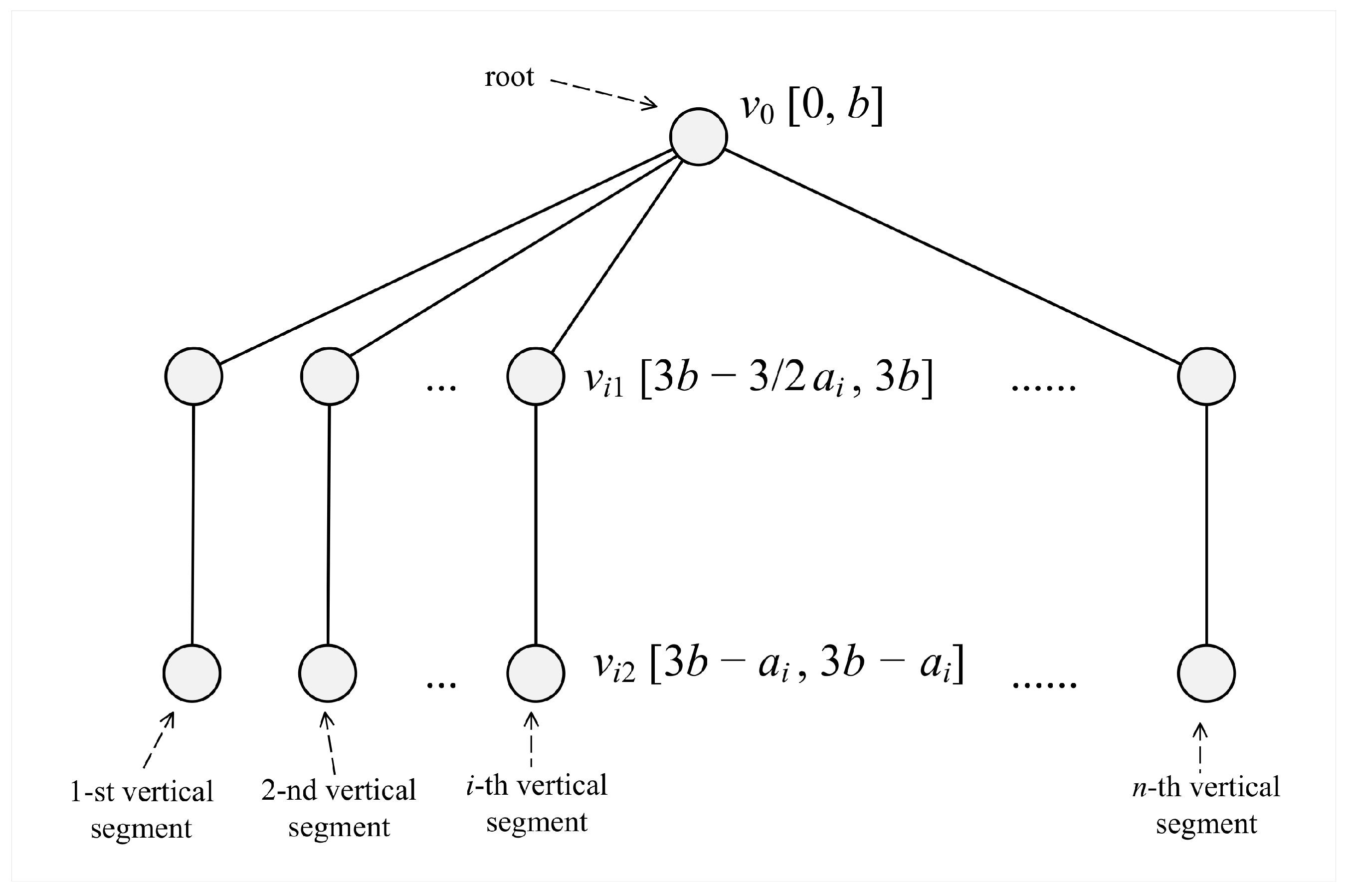
Our polynomial reduction works as follows. For a given instance of the partition problem we compute
and construct the corresponding instance of the MWIS problem shown by
Figure 1. The tree involved in our instance consists of the root
and of
n vertical segments. In the
i-th segment there are two vertices: the “upper” one
and the lower" one
. Uncertainty of vertex weights is expressed through intervals. More precisely:
The weight of is between 0 and b.
For any , the weight of is between and .
For any , the weight of is exactly .
In order to find the solution of our MWIS problem instance, one can restrict to nontrivial (non-expandable) independent sets (i.e., those that cannot be expanded with an additional vertex). Obviously, there exist two types of nontrivial independent sets:
- Type 1:
The root is included. For each the lower vertex is included.
- Type 2:
The root is not included. For each one among vertices and is included (but not both). For at least one i, the upper vertex is included.
Let us denote with the maximal regret of a min–max regret solution to our constructed MWIS problem instance, i.e., over all independent sets X of type 1 or 2. We claim the following:
The answer to the given partition problem instance is “yes" if and only if .
We prove the above claim by proving both directions.
The “if” direction. Suppose that the answer to the partition problem instance is “yes”. Then, there exists a set of indices such that . We construct the independent set X by excluding , and by choosing for and for , respectively. The worst scenario then looks as follows:
has weight b,
has weight if , and if ,
has weight if , and again if .
We compute
:
We compute
, i.e., we find the conventional optimum under scenario
by considering different solutions and identifying the best of them.
Type 1 solution has the weight
The best type 2 solution is obtained so that in each vertical segment of
T the heavier among two vertices is chosen. The obtained weight is
Thus,
Next, we apply Proposition 3 to compute the maximal regret for
X:
Since
is the minimum over all maximal regrets, it holds that
The “only if” direction. Suppose that . Then, there exists an independent set X such that . Thereby X cannot be of type 1, namely it can easily be checked that for the type 1 solution the maximal regret is equal to , which is surely . Thus, our X must be of type 2, i.e., it does not include , for any i it contains either or (but not both), and for at least one i it contains .
Let be the subset of such that if , and if . The worst scenario looks as follows:
has weight b,
has weight if , and if ,
has weight if , and again if .
We compute
:
We compute
. Thus, we search the conventional optimum under scenario
by comparing all feasible solutions.
Type 1 solution has the weight
The “heaviest" type 2 solution is obtained so that in each vertical segment of
T the heavier among two vertices is chosen. The obtained weight is
Thus,
Now, we can compute the maximal regret for
X by using Proposition 3:
From the fact that , one can conclude the following:
It cannot be true that since otherwise the left-hand part within the above would be .
It cannot be true that since otherwise the right-hand part within the above would be .
Thus, the exact equality must hold, i.e., , which means that determines a partition. □
4. Simple Algorithm
In the previous section, it has been proved that, under interval uncertainty, the min–max regret variant of the MWIS problem is NP hard, even with restriction to trees. Thus, unless P = NP, one cannot hope to find an efficient algorithm that solves the considered problem variant under the considered circumstances. The only feasible solution strategy is trying to find a good approximate algorithm.
In this section, we propose a simple approximate algorithm based on the so-called average scenario. It is the scenario where each vertex has the average weight from its interval , i.e., the (possibly non-integer) weight . Going into more details, the proposed algorithm works as follows.
For a given instance of the considered MWIS problem variant, find the average scenario.
Solve the conventional (non-robust) MWIS problem instance according to the average scenario.
The obtained solution (independent set) serves as an approximation of a min–max regret solution.
The considered algorithm is not only an approximate, but also an
approximation algorithm [
19], in the sense that it allows a constant approximation ratio. Allowing a constant approximation ratio
q means in our case the following. If
is an independent set produced by the algorithm and
is the maximal regret of a corresponding truly optimal independent set, then
. Thereby the same
q is used for all problem instances.
The described algorithm is in fact well known in the literature [
3,
8]. It can be applied in more general situations, but we believe that it is especially advantageous in our situation. Namely, its properties are then summarized by the following proposition.
Proposition 4. With restriction to trees and under interval uncertainty, the algorithm based on the average scenario finds an approximate min–max regret solution to the MWIS problem in time . Here, n is the number of vertices in the involved tree. The algorithm achieves the approximation ratio 2, and this ratio cannot be improved for trees.
Proof. In [
8], it has been proved that the considered algorithm is an approximation algorithm with a constant approximation ratio not greater than 2. The proof from [
8] is valid for general graphs, and can therefore be applied to trees. Our estimate for computing time is specific for trees, and it comes from the fact that the associate conventional problem (with the average scenario) can be solved by the linear-time algorithm from [
17]. Note that the algorithm from [
17] also works correctly when vertex weights are non-negative real numbers. To complete the proof, one must demonstrate that the general approximation ratio 2 from [
8] cannot be improved for trees. We do this by presenting our own original problem instance involving a tree, where the algorithm returns a solution
such that
is exactly equal to
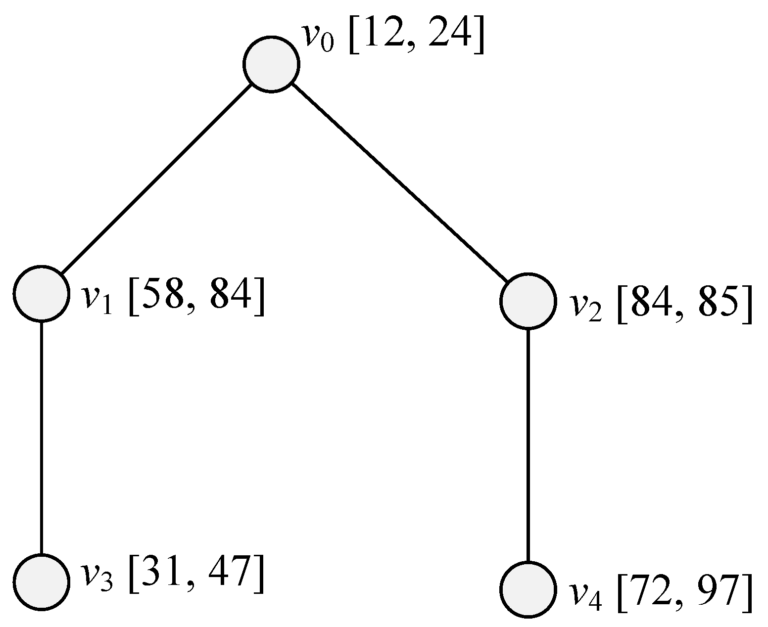
. Indeed, our problem instance is specified by
Figure 2. The figure shows a tree consisting of five vertices, each with a given interval for its weight. □
Now, the example from
Figure 2 will be explained in more detail. The vertices of the shown tree are denoted with
and
. The intervals for their weights are in turn
,
,
,
, and
. It is easy to check that there are only four nontrivial (non-expandable) independent sets, i.e.,
,
,
, and
. The weights of the five vertices according to the average scenario are in turn 18, 71, 84.5, 39, and 84.5. The weights of the four independent sets under the average scenario are in turn 123.5, 155.5, 155.5, and 123.5. Thus, our approximation algorithm can return the independent set
as its approximate solution. On the other hand, it can be checked by straightforward computation that the maximal regrets for the four independent sets are in turn 54, 26, 13, and 66. Thus, the maximal regret of our approximate solution is
, while the minimal maximal regret over all solutions is
. Thus, it really holds that
.
5. Extended Algorithm
In this section, we present an extended algorithm for solving the min–max regret variant of the MWIS problem on trees and under interval uncertainty. It is built upon the simple algorithm from the previous section. It starts with the solution obtained by the simple algorithm and tries to improve that solution through local search. Obviously, the solution obtained with the extended algorithm is never worse than the one obtained with the simple algorithm. Consequently, the extended algorithm can also be regarded as an approximation algorithm with the same or better approximation ratio.
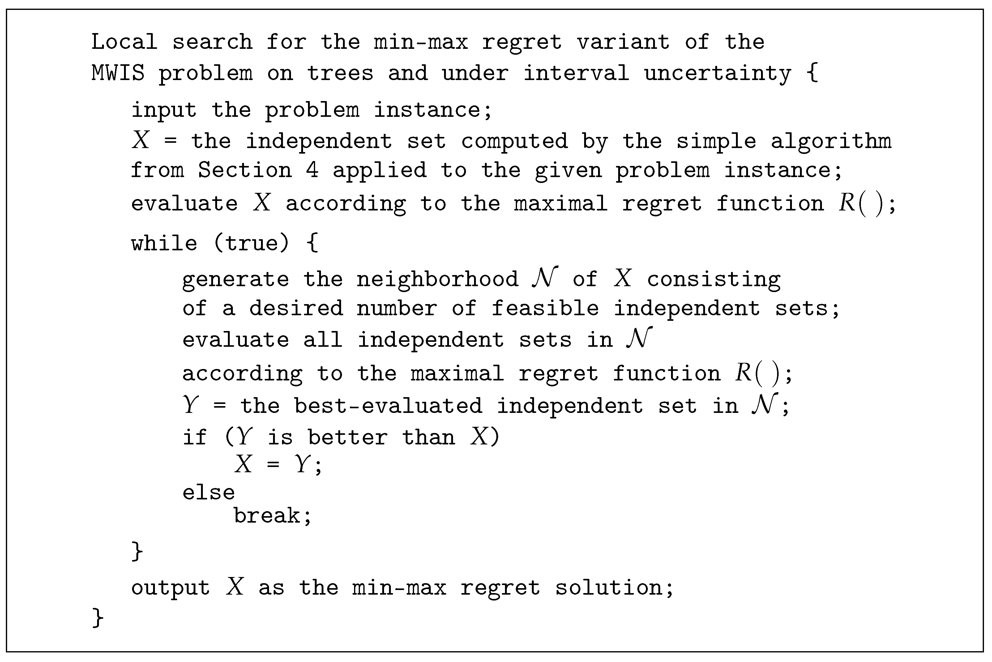
The outline of our extended algorithm is described by the pseudo-code from
Figure 3. The code obeys the standard local-search strategy developed, e.g., in [
20,
21]. Thus, for a given robust MWIS problem instance the algorithm first finds an
initial solution, i.e., a feasible independent set. In our case the initial solution is constructed by invoking the simple algorithm from the previous section. Next, the initial solution is repeatedly improved, thus producing a series of
current solutions. In each iteration, the algorithm generates a
neighborhood, which consists of various feasible perturbations of the current solution. All independent sets in the neighborhood are evaluated according to the maximal regret function
. The best member of the neighborhood (i.e., the one whose maximal regret is minimal) is identified. If that member is better than the current solution (i.e., its maximal regret is smaller), it becomes the new current solution and the algorithm resumes with a new iteration. Otherwise, the algorithm stops. The last current solution is regarded as nearly optimal (according to the min–max regret criterion).
A special property of our extended algorithm is that it considers only such solutions (independent sets) that are optimal (in the conventional sense) for some scenario. That scenario can consist either of integer or of real vertex weights. The mentioned property holds not only for the initial solution (which is optimal for the average scenario), but also for all subsequently generated current solutions and members of their neighborhoods. Consequently, each considered solution can be identified with its scenario. Modification of a current solution within local search is accomplished by perturbing the respective scenario rather than perturbing the independent set itself. Indeed, it is much easier to perturb the scenario in a feasible way. Transformation of a scenario into the corresponding independent set is accomplished by the linear-time algorithm from [
17].
Now, it will be explained in more detail how the solutions considered by our extended algorithm are evaluated and compared.
Let
be the current scenario (equivalent of the current solution). We compute the respective independent set
X by applying the algorithm from [
17]. In order to evaluate
X, we first construct its “worst” scenario
(see
Section 3), and then compute its maximal regret
according to the formula from Proposition 3:
Note that
in the above formula requires an additional call of the algorithm from [
17].
Suppose that the current scenario
has been perturbed in some way. Let
be the obtained perturbed version of
. Similarly as before, we switch from
to its corresponding independent set
Y by using the algorithm from [
17]. To evaluate
Y, we again construct its “worst" scenario
and compute its maximal regret
Thereby the value
is obtained by calling once more the algorithm from [
17].
Within one iteration of local search, usually does not need to be evaluated since its respective maximal regret is already available from the previous iteration. However, construction and evaluation of must be repeated many times in order to produce a neighborhood with a desired size. Among all instances of , one is identified whose respective Y has the smallest maximal regret . As explained earlier, the identified will become the next current scenario if its is smaller than .
Next, we have to explain how a current scenario is transformed into one of its perturbed versions . Perturbation can be done in many ways. In the present variant of the algorithm, two parameters with values between 0 and 1 are chosen in advance:
Then, for each vertex in the tree the probability that its weight will change during perturbation is equal to . The increase or decrease of weight (when it happens) is limited to the respective weight-interval width multiplied by the factor . Of course, change is done only to the extent that would not violate the original interval restriction for that particular weight. For instance, let the number of vertices be and . Let vertex weights be in the range between 1 and 50 and . Then, each of 500 vertices perturbs its weight independently one from another with probability 20%. Whenever a weight changes, the amount of change is a random number between of 50 (i.e., between −5 and +5).
Let us say something about computational complexity of the extended algorithm. Construction of an instance of
is done in time linear with respect to the tree size
n. Evaluation of
or of any instance of
requires two invocations of the (linear-time) algorithm from [
17]. Consequently, for a constant neighborhood size, the computing time of an iteration is linear with respect to
n.
Regarding space complexity, the extended algorithm does not require a lot of memory. It only needs to store information about the tree and about the current best solution. Iterations do not require new space because a new better solution replaces the current best solution. Consequently, the total space requirement is linear with respect to the tree size n.
6. Experimental Evaluation
In this section, we present our experimental evaluation of the two algorithms from
Section 4 and
Section 5, respectively. It would be nice if the algorithms could be tested on some established benchmark instances for robust variants of the MWIS problem. However, to the best of our knowledge, such benchmarks do not exist, especially not on trees or with interval uncertainty. Therefore, we have generated our own three test groups, the first comprising 30, the second 120, and the third again 120 robust MWIS problem instances. We call the three groups
small,
medium-sized and
large instances, respectively.
Here follows a more detailed description of our test data. Of course, all instances in our test groups are posed on trees, and uncertainty of their vertex weights is expressed by intervals. Additionally, all instances are meant to be solved according to the min–max regret criterion. Some parameters, such as numbers of vertices, bounds for tree outspread or bounds for vertex weights, are chosen in advance. The remaining details are generated randomly. Indeed:
Small instances are based on random trees consisting of vertices, where each vertex has at most 3 children. The lower bound for a vertex weight is always 1, and the upper bound is at most 5.
Medium-sized instances comprise random trees with vertices. There are four subgroups of 30 instances, characterized by different outspread bounds. More precisely, in the first subgroup, each vertex in a tree can have at most three children, while the maximum number of children in the second, third and fourth subgroup is 5, 10 and 15, respectively. Regardless of a subgroup, the range for a vertex weight is from 1 to at most 50.
Large instances contain random trees having vertices. Again, there are four subgroups of 30 instances, characterized by different outspread bounds. Depending on a subgroup, a vertex can have at most 3, 5, 10 and 15 children, respectively. In all four subgroups, vertex weights are in the interval from 1 to at most 1000.
The instances from the first group may look rather small (only 20 vertices). However, according to our experience, they are in fact the largest ones that can be solved to optimality by using a straightforward mathematical model and a general-purpose software such as CPLEX [
22]. Indeed, our straightforward model is based on constraints corresponding to extremal scenarios [
12]. For 20 vertices, there are as many as
1,048,576 such constraints. All of them are explicitly listed in the model, thus reaching the limits of CPLEX capabilities. It is true that some larger problem instances could still be solved exactly by more sophisticated models and algorithms [
3], where only a small part of the constraint set is initially used and then gradually extended. However, exploration of such methods is beyond the scope of this paper.
The simple algorithm from
Section 4, as well as the extended algorithm from
Section 5, have been implemented in the Java programming language. Both implementations also comprise the linear-time algorithm from [
17] as a subroutine. In the second implementation, the two parameters
and
(see
Section 5), as well as the neighborhood size for local search, can freely be chosen and specified as input data. To measure accuracy of our approximation algorithms (at least on small instances), we have also used the previously mentioned CPLEX package. All software has been installed on the same computer, with an Intel Core I7-975OH @2.60 GHz processor and 16 GB of RAM, running a 64-bit operating system. Our original source code is available in the same repository as the problem instances.
In the experiments we have solved each problem instance from each of the three test groups by both approximation algorithms. The small instances (first test group) have additionally been solved to optimality by CPLEX (with the straightforward mathematical model and explicitly listed constraints). The medium-sized and large instances (second and third test group) have repeatedly been solved by the extended algorithm, each time with a different combination of parameters and . In all experiments, the neighborhood size within local search has been fixed to 100.
For each solution we have recorded the obtained maximal regret
and the corresponding computing time. The results of the experiments are summarized in
Table 1,
Table 2 and
Table 3. Thereby
Table 1 corresponds to small,
Table 2 to medium-sized, and
Table 3 to large instances.
Let us now take a closer look at
Table 1. Each row of the table corresponds to one of the 30 small problem instances. For each instance, its identifier is shown (comprising its number of vertices, tree outspread bound and bound for vertex weights). Additionally, there is the (truly minimal) maximal regret obtained by CPLEX and the maximal regrets computed by the simple and the extended algorithm, respectively. The results of the extended algorithm have been obtained with the parameter values
and
. Note that for 21 out of 30 instances, the simple algorithm reaches the same maximal regret as CPLEX. For 8 out of 9 remaining instances the extended algorithm improves the result obtained by the simple algorithm, thus reaching again the minimal maximal regret found by CPLEX. There is only one instance where both our approximation algorithms fail to produce the optimal solution. For each approximate solution the table also shows its empirical approximation ratio, i.e., the quotient of its maximal regret versus the minimal maximal regret. The average approximation ratio is 1.12 for the simple algorithm, and 1.01 for the extended algorithm. This is much better than the worst-case approximation ratio 2 from Proposition 4.
Next, we will explain in more detail
Table 2. Each row of that table corresponds to one subgroup of 30 medium-sized problem instances with a particular tree outspread bound. All instances within the same subgroup have identifiers with the same prefix, as shown in the first column of the table. The prefix comprises the number of vertices (i.e., 500), the tree outspread bound (i.e., at most 3, 5, 10 and 15 children per vertex, respectively), and the bound for vertex weights (between 1 and at most 50).
Table 2 does not contain truly optimal solutions since the instances are too large to be solved exactly by CPLEX. Instead, only the average maximal regrets obtained by the two approximation algorithms are shown, together with their corresponding average computing times in milliseconds. Additionally, there are the average improvements achieved by the extended algorithm versus the simple algorithm, and the average slowdowns of the extended algorithm versus the simple algorithm. Thereby the improvement for a particular problem instance is computed as the difference of the two corresponding maximal regrets divided by the larger maximal regret. Similarly, the slowdown for a particular problem instance is obtained as the larger computing time divided by the smaller computing time. All values for individual problem instances (maximal regrets, times, improvements, slowdowns) are averaged over each subgroup of 30 problem instances.
Table 2 also presents the concrete values of parameters
and
used within the extended algorithm. Thereby, for each subgroup of problem instances, different values have been chosen. In fact, in our experiments, we have tested various combinations of
and
:
The values shown in the table are those that assured the largest average improvements for particular subgroups. One can see that the extended algorithm always improves the results of the simple algorithm, but this improvement is paid by much longer computing time.
From
Table 2, one can also observe that improvement usually becomes better (larger) when tree outspread becomes smaller. The best improvement is achieved on trees whose vertices have up to 5 children, while the worst improvement occurs when vertices can have 15 children. On the other hand, slowdowns behave in the opposite way, i.e., they are better (smaller) for trees with larger outspread. Indeed, the best slowdown is accomplished if vertices can have 15 children, and the worst slowdown is for trees whose vertices do not have more than three children. This behavior can be explained as follows: when the total number of vertices is fixed, trees with larger outspread have less levels. And less levels means less independent sets, so there are less combinations to try. The extended algorithm will finish faster because the generated neighborhoods will contain small numbers of new independent sets.
Finally, let us say something about
Table 3. It deals with large problem instances, but otherwise is analogous to
Table 2. Again, one can see the average improvements and slowdowns of the extended algorithm versus the simple algorithm depending on the tree outspread bound. There is a similar correlation of improvement or slowdown versus tree outspread as in
Table 2. Compared to
Table 2, average improvements are roughly the same, but they are achieved with much smaller values for
. In fact, average improvements for medium-sized problem instances are optimal when
, while for large instances they are optimal when
. These two intervals do not have intersection. The perceived phenomenon regarding values of
can be explained in the following way. In order to get a new independent set, we need to change the current independent set, but the change must not be too drastic since the current independent set is already a good solution. Large problem instances have much more vertices, thus the same total amount of change is obtained with a smaller value of
. If one compares values of
from
Table 2 and
Table 3, one can see that there is no such big difference as for values of
. Thus, for both medium-sized and large problem instances, changes of vertex weights (when they occur) should have similar intensity.
It is interesting to note that average improvements in
Table 2 and
Table 3 stay similar, although large problem instances contain 20 times more vertices than medium-sized instances. In more detail, average improvements for medium-sized instances are slightly better on subgroups with five and 15 children, while for large instances they are slightly better on subgroups with three and 10 children. On the other hand, average slowdown does not increase 20 times on large instances. In fact, it increases between 2.4 and 12.5 times. The greatest increase is for trees with small outspread and it becomes smaller as the outspread grows. The observed nonlinearity assures that the extended algorithm can be used for very large trees, even larger than those involved in our experiments.
7. Conclusions
In this paper, we have studied two robust variants of the MWIS problem, i.e., the max–min and the min–max regret variant. Both of them have been posed on trees. Uncertainty has been restricted to vertex weights and represented by intervals. We have been interested in complexity aspects, as well as in algorithmic aspects.
On one hand, we have observed that the considered max–min variant can easily be solved in linear time, by an algorithm originally intended for the conventional (non-robust) variant. On the other hand, we have proved that the corresponding min–max regret variant is NP-hard, which justifies its approximate solution. Consequently, the algorithmic part of the paper has been devoted to two approximation algorithms for the min–max regret variant. They are called simple and extended algorithm, respectively. The first of them gives the solution based on the so-called average scenario, while the second one tries to improve that solution by local search.
The simple algorithm runs on our problem instances in linear time. However, its general worst-case approximation ratio 2 cannot be improved in spite of restriction to trees. Still, the experiments presented in the paper clearly indicate that the corresponding average approximation ratio, at least on small trees, is much better, i.e., slightly larger than 1. Regarding the extended algorithm, the experiments have confirmed that it produces even better solutions than the simple algorithm. Indeed, on large trees it improves accuracy of the simple algorithm up to 7%. However, this improvement in accuracy is paid by much larger computing time.
It is important to note that the min–max regret variant of the MWIS problem under interval uncertainty is fairly demanding in computational sense, even when restricted to trees. Namely, the number of implicitly given scenarios that must be considered grows exponentially with the number of vertices. According to our experience, state-of-the-art computers with available software are able to find exact solutions only on rather small trees having few dozens of vertices. At this moment, our approximation algorithms seem to be the only known solution methods that are suitable for larger trees.
In our future work, we will try to speed up the extended algorithm by parallel processing. It can be done since each iteration of the involved local search consists of parallelizable computations. Our second plan for the future is to develop an iterative exact algorithm for the min–max regret variant. The idea is to use a mathematical model, where an initial (small) constraint set is iteratively extended as long as the corresponding solution is infeasible. We expect that such an algorithm will be able to find exact solutions for problem instances of moderate size.


