Exact Solutions of Boundary Layer Equations in Polymer Solutions

Abstract

The paper presents new exact solutions of equations derived earlier. Three of them describe unsteady motions of a polymer solution near the stagnation point. A class of partially invariant solutions with a wide functional arbitrariness is found. An invariant solution of the stationary problem in which the solid boundary is a logarithmic curve is constructed.

1. Introduction

The theory of motion of a viscous fluid based on the Navier–Stokes equations is unable to describe the flow of a weak aqueous polymer solution, as the Navier–Stokes theory does not take into account the properties that the equilibrium state in the liquid, corresponding to the rheological Newton’s law, establishes, not instantly, after a change in external conditions, as required by this law, but after some time, characterized by the value of the relaxation time [1]. These relaxation properties of the liquid dramatically differ for water and polymer solutions. One of the models applied for the theoretical description of the dynamics of polymer solutions is the Pavlovskii model [1]:

$$\frac{d\mathbf{v}}{dt}=-\frac{1}{\rho }\nabla p+\nu \Delta \mathbf{v}+\kappa \frac{d\Delta \mathbf{v}}{dt},div\mathbf{v}=0,$$

(1)

where $\mathbf{v}$ is the velocity vector, p is the pressure, $\rho$ is the fluid density, $\nu$ is the kinematic viscosity and $\kappa$ is the normalized relaxation viscosity [2], ${\displaystyle \frac{d}{dt}=\frac{\partial }{\partial t}+\mathbf{v}·\nabla }$. The parameters $\nu$ and $\kappa$ are considered positive constants.

The above system of equations differs from the Navier–Stokes equations due to the presence of the term ${\displaystyle \kappa \frac{d\Delta \mathbf{v}}{dt}}$, which describes the relaxation properties of the fluid. In the case of very weak relaxation properties (for $\kappa$ close to zero), and also in the case when the motion of the liquid has a steady-state character (the total derivative of the strain rate tensor with respect to time is equal to zero), this additional term vanishes, in which case Equation (1) coincides with the Navier–Stokes equations.

The model (1) of the motion of weakly concentrated aqueous polymer solutions has been confirmed by experimental studies in [3]. The problem of the solvability of the initial-boundary value problems of the Pavlovskii model (Equation (1) with no-slip conditions on the boundary of the flow region was studied in [4,5], and in Chapter 4 of the monograph [6]. A similar problem, but with slip conditions on the boundary, was studied in [7]. Stationary solutions of system (1) were analyzed in [8,9]. The group properties of Equation (1) and the construction of their exact solutions were studied in [2,10,11,12].

For describing laminar flows in the vicinity of walls, the boundary layer theory has been developed. The derivation of the boundary layer equations is based on simplifications of the Navier–Stokes equations. Equations of a plane unsteady boundary layer in an aqueous polymer solution near a rectilinear wall were derived in [13]. The equations of the laminar boundary layer, based on the Pavlovskii model, and in the case of plane motion $\mathbf{v}=(u,v,0)$, are the following:

$$\begin{array}{c}{u}_t+u{u}_x+v{u}_y=-p_x+\chi u_{yy}+u_{tyy}+u{u}_{xyy}+v{u}_{yyy},\\ u_x+v_y=0,p_y=0,\end{array}$$

(2)

where there is a single dimensionless parameter $\chi$. This parameter is defined by the relation,

$$\chi =\frac{\nu l}{V\kappa },$$

where l is the characteristic longitudinal scale of length and V is the characteristic velocity scale of the oncoming flow.

The integration of the third equation of (2) provides an arbitrary function $p(x,t)$. The complete group classification of system (2) with respect to this arbitrary element $p(x,t)$ was performed in [13]. It was shown that the kernel of admitted Lie algebras is defined by the generators:

$$X_h=h{\partial }_y+(u{h}_x+h_t){\partial }_v,$$

where $h(x,t)$ is an arbitrary function. An extension of the kernel occurs for particular functions $P(x,t)=p_x(x,t)$. If $P(x,t)=e^{kt}F\left(x{e}^{-kt}\right)$, where k is constant and $g^{″}\ne 0$, then the extension of the kernel of admitted Lie algebras is defined by the generator:

$$k(u{\partial }_u+x{\partial }_x)+{\partial }_t.$$

If $P(x,t)=xg\left(t\right)$, then the extension of the kernel of admitted Lie algebras depends on $g^{\prime }$. For $g^{\prime }\ne 0$, the extension is defined by the generators:

$$u{\partial }_u+x{\partial }_x,g_i^{\prime }{\partial }_u+g_i{\partial }_x,(i=1,2),$$

(3)

where $g_1\left(t\right)$ and $g_2\left(t\right)$ compose a fundamental system of solutions of the second-order ordinary differential equation ${\xi }^{″}+\xi g=0$. For $g^{\prime }=0$, one can assume that $g=0$ by virtue of an equivalence transformation, and the generators (3) are extended by the additional admitted generator ${\partial }_t$. The paper [13] also contains a number of exact solutions of system (2).

The knowledge of an admitted Lie group allows for constructing invariant and partially invariant solutions. For this purpose, one needs to classify the admitted Lie algebra by constructing subalgebras. For a given subalgebra, one finds invariants [14,15]. Using the invariants, one defines an invariant [14,15] or a partially invariant [14] solution.

The present paper is devoted to constructing invariant and partially invariant solutions of system (2). It is organized as follows.

Section 2 is devoted to three new nonstationary solutions of the system of Equation (2), describing the motion of an aqueous polymer solution near a stagnation point. Section 3 deals with the class of partially invariant solutions possessing two arbitrary functions of single arguments. Section 4 provides a solution of the boundary layer equations near a logarithmic curve. Section 5 presents the Conclusions.

2. Nonstationary Motions near a Stagnation Point

The problem of fluid motion near a stagnation point is one of the classical problems of hydrodynamics. An exact solution of the Navier–Stokes equations, describing a steady flow near the stagnation point, was obtained in [16,17]. The corresponding nonstationary problem and the stationary solutions of the problem of the motion of a polymer solution near stagnation points were studied and investigated in [18,19,20]. This section provides three exact solutions of the nonstationary problem of Equation (2).

The first solution is obtained by using the method of differential constraints [21,22].

Consider a system of equations of a plane unsteady flow of the boundary layer of an aqueous polymer solution (2):

$${(u-u_{yy})}_t+u{(u-u_{yy})}_x+v{(u-u_{yy})}_y=-p_x+\chi u_{yy},u_x+v_y=0.$$

(4)

Add to system (4) the differential constraint:

$${(u-u_{yy})}_y=0.$$

(5)

The solution of the latter equation, satisfying the no-slip condition at $y=0$, and bounded as $y\to \infty$, has the form:

$$u(x,y,t)=c(x,t)\left(1-exp(-y)\right),$$

(6)

where $c(x,t)$ is an arbitrary function. Substitution of the expression (6) into the first equation of system (4) leads to the relations:

$$c_x=\chi ,c_t+c{c}_x=-p_x,$$

from which one has:

$$c=\chi x+f,p=-(\chi +f^{\prime })x-{\left(\chi x\right)}^2/2,$$

(7)

where $f\left(t\right)$ is an arbitrary function and $f^{\prime }$ denotes its derivative. The second equation of system (4), together with the no-slip condition, gives the expression for the function v,

$$v=\chi (-y+1-exp(-y\left)\right).$$

(8)

In the case $f=0$, Formulas (6)–(8) describe a steady flow near the stagnation point $x=0,y=0$. For an arbitrary $f\left(t\right)$, the stagnation point has the coordinates $x=-f\left(t\right)/\chi ,y=0$, and the flow region is the quadrant $x>-f\left(t\right)/\chi ,y>0$ in the $xy$-plane. In this case, the condition $u>0$ is satisfied in the flow region, which is dictated by the initial assumptions during deriving system (4) from the equations of the Pavlovskii model.

Equations (4) admit the generalized Galilean transformation:

$$\tilde{t}=t,\tilde{x}=x+g\left(t\right),\tilde{y}=y,\tilde{u}=u+f\left(t\right),\tilde{v}=v,\tilde{p}=p-x{f}^{\prime }\left(t\right),$$

where $g\left(t\right)$ is an antiderivative of the function $f\left(t\right)$. Applying the indicated transformation in Formulas (6)–(8), we arrive at a stationary solution of system (4), noted above. Thus, the functional arbitrariness in solution (6)–(8) has the group-theoretical nature.

The other two solutions are partially invariant solutions of system (2). Further exact solutions of Equation (11) are then constructed using the method of invariant subspaces [23].

System (4) admits a group with the generators

$${\partial }_x,t{\partial }_x+{\partial }_u.$$

(9)

There are no solutions of system (4) invariant with respect to this group, but there are partially invariant solutions. The general form of such a solution, symmetric with respect to the x-axis is

$$u=xf(y,t),v=-{\int }_0^{y}f(z,t)dz.$$

(10)

Solution (10) corresponds to the pressure distribution $p=-x^{2}q\left(t\right)/2$, where the function $q\left(t\right)$ is given, and is considered in the domain $x\ge 0,y\ge 0,t\ge 0$. The function $f(y,t)$ satisfies the equation:

$${(f-f_{yy})}_t+f(f-f_{yy})-{(f-f_{yy})}_y{\int }_0^{y}f(z,t)dz=q+\chi f_{yy}.$$

(11)

A physical meaning has solutions for which $f\ge 0$. The velocity components have to satisfy the no-slip condition at $y=0$. For the component v, this condition is satisfied by virtue of (10). Requiring that $u=0$ at $y=0$, we arrive at the condition:

$$f(0,t)=0,t\ge 0.$$

(12)

Equation (11) has two two-parameter families of exact solutions satisfying condition (12).

One of these families has the form:

$$f(y,t)=l\left(t\right)\left(1-cos(y/s(t\left)\right)\right),$$

(13)

where the functions $l\left(t\right)$ and $s\left(t\right)$ are solutions of the Cauchy problem:

$$\frac{dl}{dt}=-\frac{1}{1+s^2}\left((3+2s^2)l^2+\chi l\right),\frac{ds}{dt}=-ls,t>0,l\left(0\right)=l_0>0,s\left(0\right)=s_0>0.$$

(14)

In this case, the following condition should be satisfied:

$$q=-\frac{\chi l}{1+s^2}+\frac{l^2}{s^2(1+s^2)}.$$

(15)

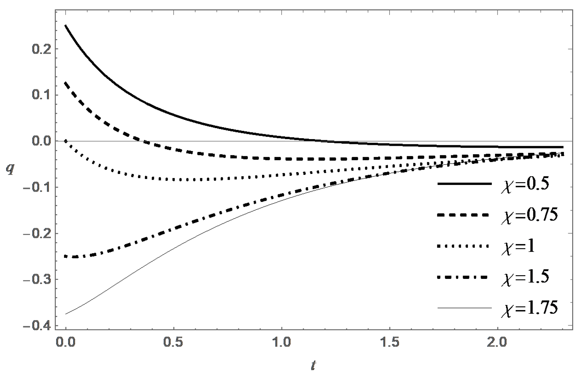
Thus, the function $q\left(t\right)$ is determined a posteriori, after finding a solution to the Cauchy problem (14). Depending on the parameters $l_0$, $s_0$ and $\chi$, this function may change sign over time. Figure 1 presents graphs of the function $q\left(t\right)$ for different values of the parameter $\chi$.

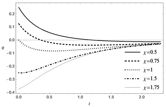
Figure 1. The function q obtained by numerically solving the Cauchy problem (14), where $l_0=1$, $s_0=1$ for various values of $\chi$.

A characteristic feature of solution (13) of Equation (11) is that the function f has no limit when $y\to \infty$. Figure 2 presents graphs of the function $f\left(t\right)$ at different time. It follows from the second equation of (14) that the function $s\left(t\right)$ decreases monotonically, and the following estimates $0<s<s_0$ are valid for $t>0$. Using simple comparison theorems, this allows one to obtain two-sided estimates $0<l_{-}\le l\le l_{+}$. The functions $l_{-}\left(t\right)$ and $l_{+}\left(t\right)$ satisfy the equations $d{l}_{-}/dt=-3l_{-}^2-\chi l_{-}$ and $d{l}_{+}/dt=-2l_{+}^2-\chi {(1+s_0^2)}^{-1}{l}_{+}$, and the same initial conditions $l_{-}\left(0\right)=l_{+}\left(0\right)=l_0$. Hence, the estimate $l=O\left(exp(-ct)\right)$ for $t\to \infty$ follows, where $c=\chi {(1+s_0^2)}^{-1}$. In turn, the existence of the limit ${\displaystyle \underset{t\to \infty }{lim}s\left(t\right)=s_{\infty }>0}$ follows from it.

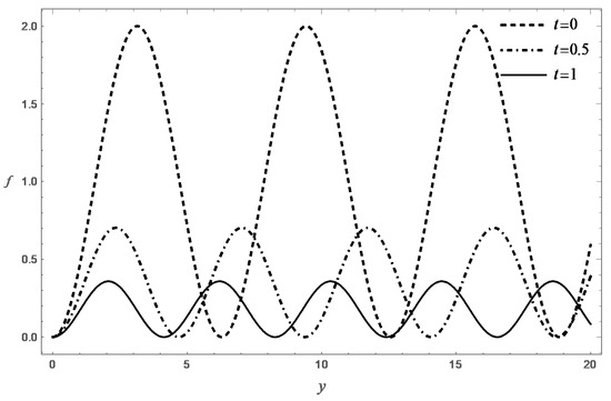
Figure 2. The function f obtained by numerically solving the Cauchy problem (14), where $l_0=1$, $s_0=1$ and $\chi =1$ for various times t.

The same estimate, together with (15), shows that, starting from some $t_{*}$, the function $p_x=-xq$ takes positive values for $x>0$. In the classical theory of the boundary layer, the unfavorable nature of the pressure distribution makes it impossible to extend a solution of the boundary layer equations to large values of x, which is interpreted as a separation of the boundary layer. In our example, such a phenomenon does not occur due to the fact that $q\to 0$, when $t\to \infty$, and the motion eventually stabilizes to the rest state.

The second class of solutions is defined by the relation:

$$f(y,t)=m\left(t\right)\left(1-exp(-y/s(t\left)\right)\right),$$

(16)

where the functions $m\left(t\right)$ and $s\left(t\right)$ are solutions of the Cauchy problem:

$$\frac{dm}{dt}=-\frac{2-s^2}{1-s^2}{m}^2-\frac{\chi m}{1-s^2},\frac{ds}{dt}=-ms$$

(17)

with the initial conditions:

$$m\left(0\right)=m_0>0,s\left(0\right)=s_0>0.$$

(18)

After solving the Cauchy problem (17) and (18), then $q\left(t\right)$ is determined from the relation $q=dm/dt+m^2$, which, due to (17), can be rewritten as:

$$q=-\frac{1}{1-s^2}(m^2+\chi m).$$

(19)

In addition, there is an isolated solution of the form (16), in which $m=\chi ,s=1$.

Further, two cases are considered: (A) $s_0<1$, and (B) $s_0>1$. Passing in system (17) to the $(m,s)$ phase plane, we obtain the linear equation:

$$\frac{dm}{ds}=\frac{2-s^2}{s(1-s^2)}m+\frac{\chi }{s(1-s^2)}.$$

(20)

In case (A), the solution of the latter equation under the condition $m=m_0$ for $s=s_0<1$ has the form:

$$\begin{array}{ccc}\hfill m& =& {\displaystyle m_0\frac{s^2\sqrt{1-s_0^2}}{s_0^2\sqrt{1-s^2}}+\frac{\chi }{2}\left(\frac{s^2\sqrt{1-s_0^2}}{s_0^2\sqrt{1-s^2}}-1\right)}\hfill \\ \hfill & +& {\displaystyle \frac{\chi s^2}{4\sqrt{1-s^2}}ln\left(\frac{(1+\sqrt{1-s_0^2})(1-\sqrt{1-s^2})}{(1-\sqrt{1-s_0^2})(1+\sqrt{1-s^2})}\right).}\hfill \end{array}$$

(21)

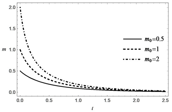
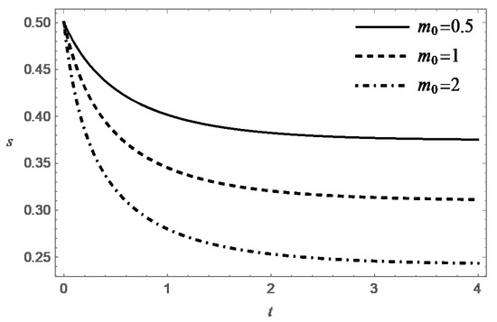
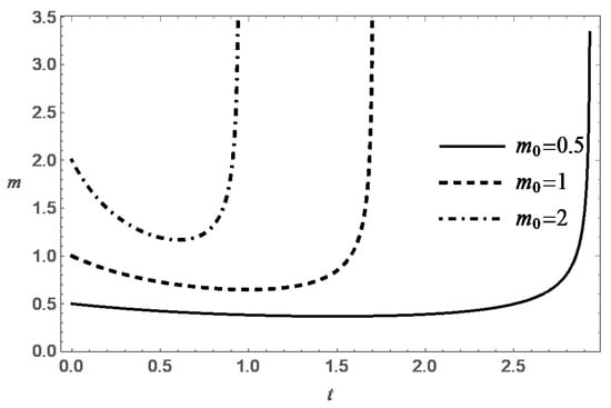
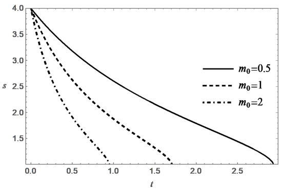
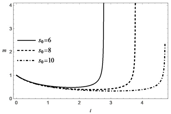
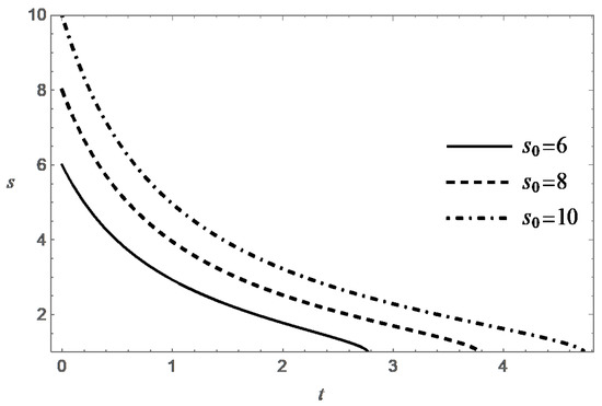
There exists $s_{*}$ such that the function $m\left(s\right)$ at $m_0>0$ takes positive values for $s\in (s_{*},s_0)$, and is monotonic and ${\displaystyle \underset{s\to s_{*}}{lim}m\left(s\right)=0}$. Substituting expression (21) into the second equation of system (17), one obtains a representation for the function $s\left(t\right)$ in the form of a quadrature. Notice that the function $m\left(s\right)$ at $s\to s_{*}$ has the form

$$m\left(s\right)=\frac{\chi }{s_{*}(1-s_{*}^2)}(s-s_{*})+O\left({(s-s_{*})}^2\right).$$

Hence, it follows that:

$$s\left(t\right)=s_{*}+O\left(exp\left(-\frac{\chi t}{1-s_{*}^2}\right)\right),t\to \infty .$$

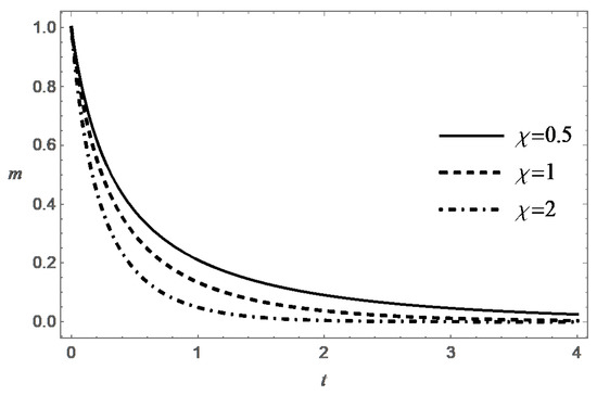
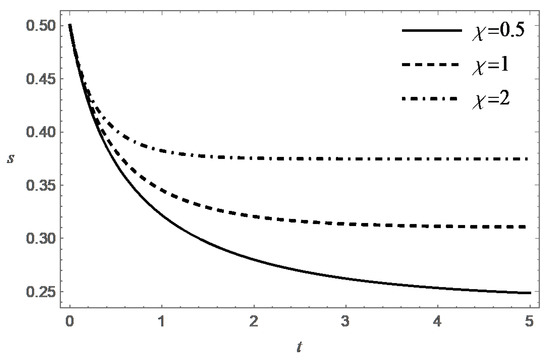
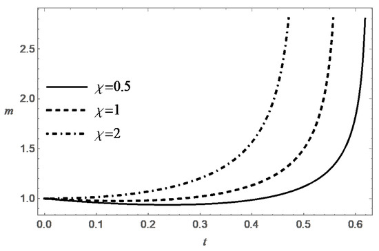
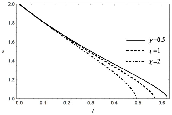
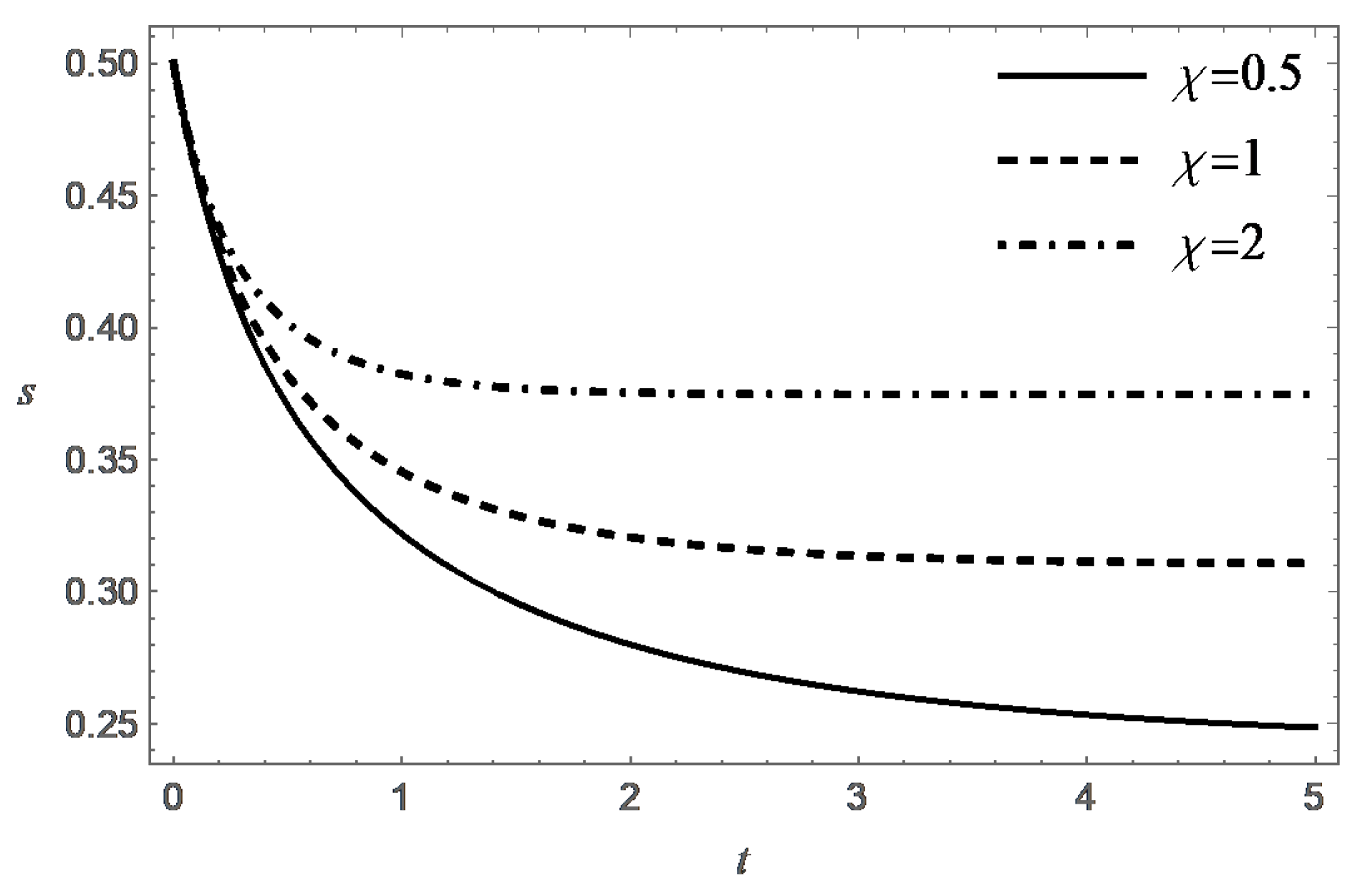
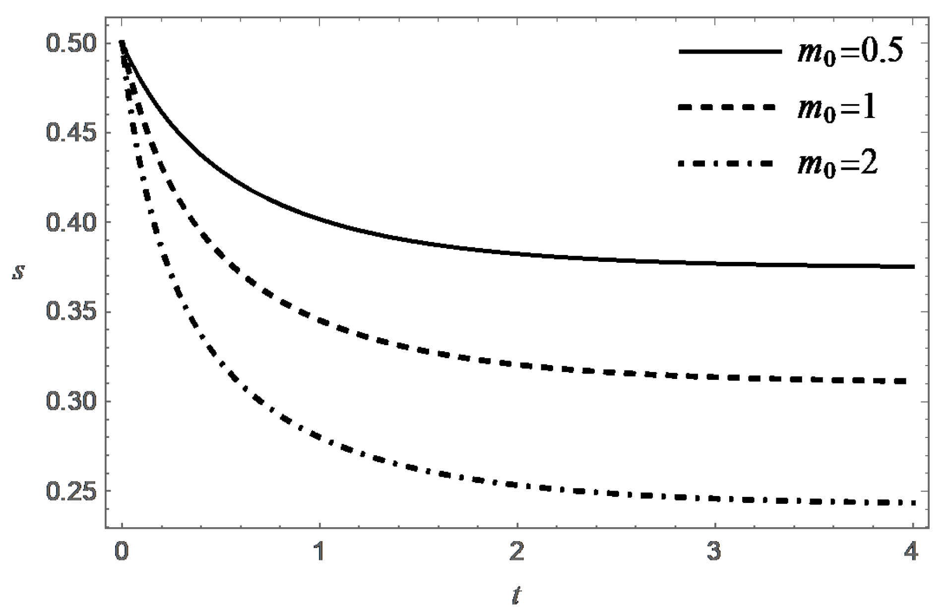
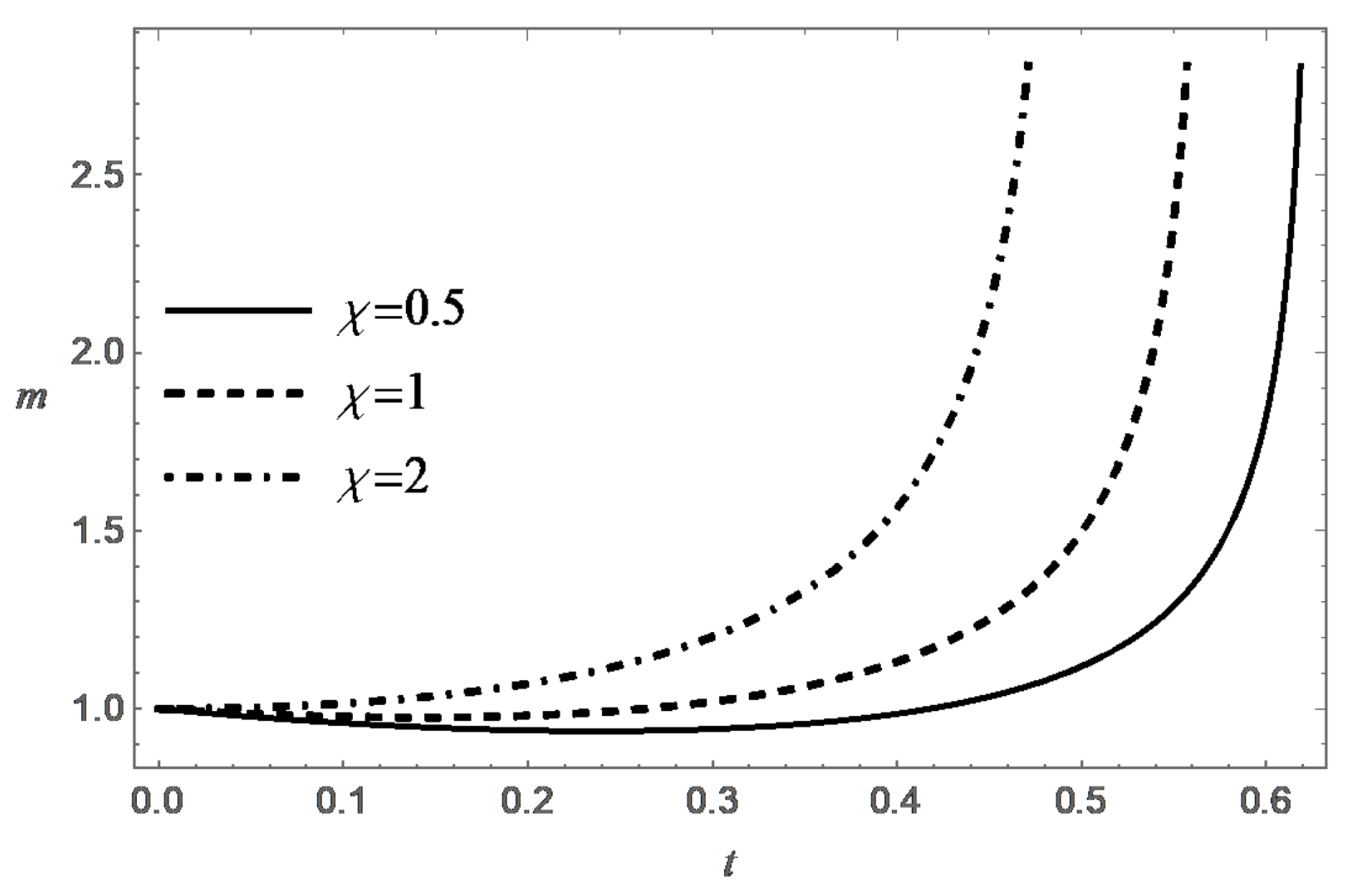
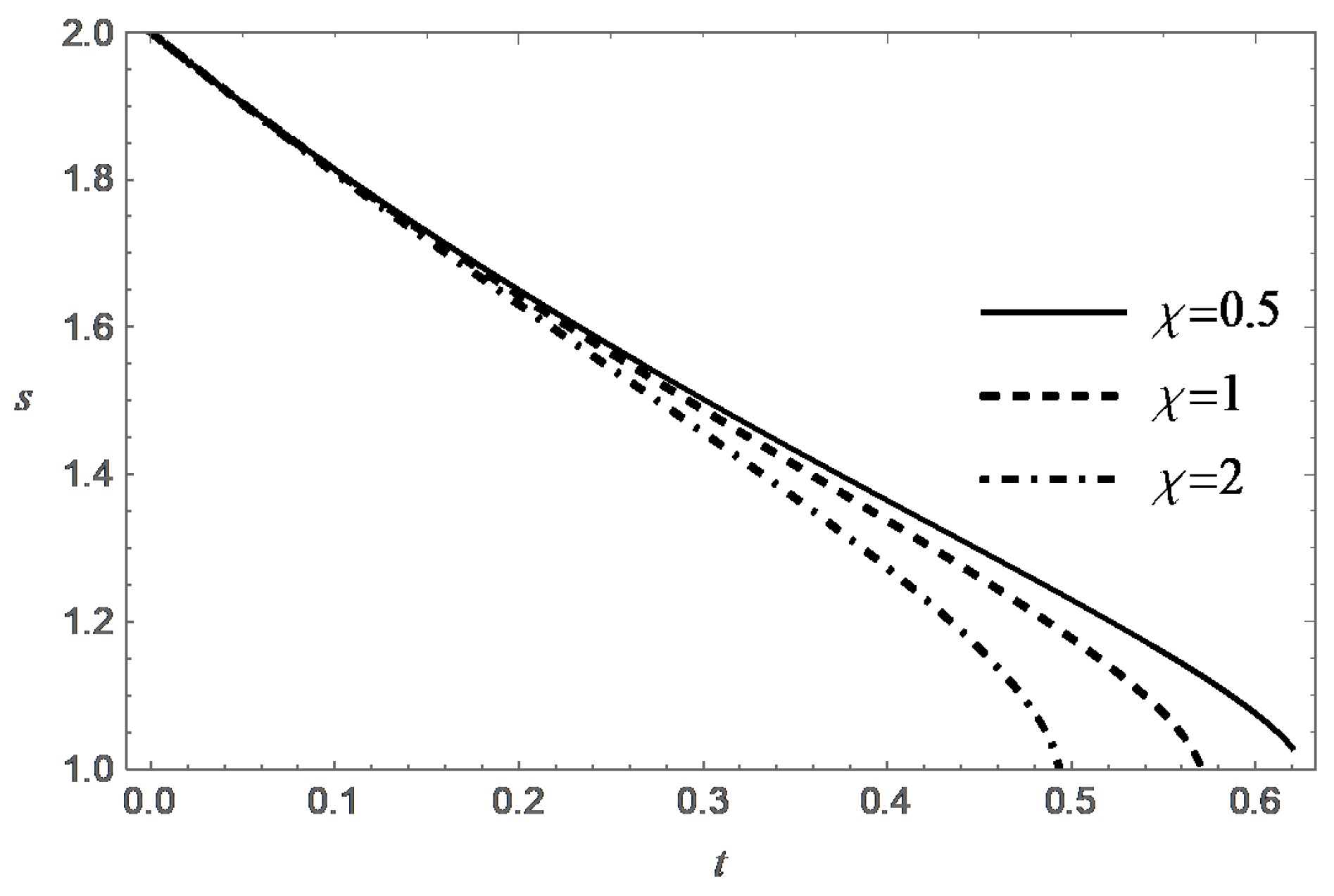
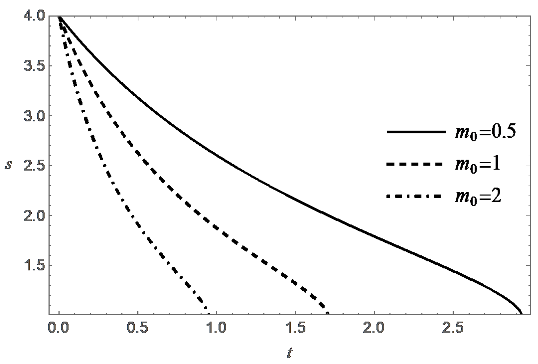
Thus, the function $s\left(t\right)$ decreases monotonically with increasing t, and $s\to s_{*}$ at an exponential rate when $t\to \infty$. Figure 3, Figure 4, Figure 5 and Figure 6 present behavior of the functions m and s in the case (A) for different values of $\chi$ and $m_0$.

Figure 3. The function m obtained by numerically solving the Cauchy problem (17) and (18) in case (A), where $m_0=1$, $s_0=0.5$ and for various values of $\chi$.

Figure 4. The function s obtained by numerically solving the Cauchy problem (17) and (18) in case (A), where $m_0=1$, $s_0=0.5$ and for various values of $\chi$.

Figure 5. The function m obtained by numerically solving the Cauchy problem (17) and (18) in case (A), where $\chi =1$, $s_0=0.5$ and for various values of $m_0$.

Figure 6. The function s obtained by numerically solving the Cauchy problem (17) and (18) in case (A), where $\chi =1$, $s_0=0.5$ and for various values of $m_0$.

In case (B) ($s_0>1$), the equation on the phase plane can be conveniently rewritten in the form

$$\frac{dm}{ds}=\frac{s^2-2}{s(s^2-1)}m-\frac{\chi }{s(s^2-1)}.$$

(22)

The solution of Equation (22) under the condition $m=m_0$ for $s=s_0>1$ is given by the formula:

$$m=m_0\frac{s^2\sqrt{s_0^2-1}}{s_0^2\sqrt{s^2-1}}+\frac{\chi }{2}\left(\frac{s^2\sqrt{s_0^2-1}}{s_0^2\sqrt{s^2-1}}-1\right)+\frac{\chi s^2}{2\sqrt{s^2-1}}\left(arccos\frac{1}{s_0}-arccos\frac{1}{s}\right).$$

(23)

It can be shown that the solution of Equation (22) is destroyed in finite time for any $m_0>0,s_0>1$. According to (23), one has: $m\ge m_0{s}^2{(s_0^2-1)}^{1/2}{s}_0^{-2}{(s^2-1)}^{-1/2}$. This leads to the inequality

$$\frac{ds}{dt}\le -m_0\frac{s^2\sqrt{s_0^2-1}}{s_0^2\sqrt{s^2-1}},$$

which is equivalent to the following:

$$\frac{\sqrt{s^2-1}}{s^3}\frac{ds}{dt}\le -\frac{m_0\sqrt{s_0^2-1}}{s_0^2}.$$

Integrating the latter inequality, one gets for $t\ge 0$:

$$\frac{\sqrt{s^2-1}}{2s^2}-\frac{\sqrt{s_0^2-1}}{2s_0^2}+\frac{1}{2}\left(arccos\frac{1}{s}-arccos\frac{1}{s_0}\right)\le -m_{0}t\frac{\sqrt{s_0^2-1}}{s_0^2}.$$

Taking into account that the function $s\left(t\right)$ decreases with increasing t, one can strengthen this inequality:

$$\sqrt{s^2-1}<-2m_{0}t\sqrt{s_0^2-1}+\sqrt{s_0^2-1}+s_0^{2}arccos\left(s_0^{-1}\right),$$

whence it follows that the lifetime $t^{*}$ of the solution to problem (22), (18) under the condition $s_0>1$ does not exceed the value:

$$T=\frac{\sqrt{s_0^2-1}+s_0^{2}arccos\left(s_0^{-1}\right)}{2m_0\sqrt{s_0^2-1}}.$$

(24)

Note that this expression for T does not contain the parameter $\chi$. At the same time $s\to 1,m\to \infty$, and simultaneously $q\to \infty$, when $t\to t^{*}$. Thus, the conditions $m_0>0,s_0>1$ are sufficient conditions for the destructing the solution of the problem (17), (18) in finite time.

It was shown above that, under natural physical constraint $m_0>0$, the condition $s_0>1$ is also a necessary condition for destruction. According to (24), the value of T increases monotonically with increasing t, and $T=\pi s_0/\left(4m_0\right)+O\left(1\right)$, when $s_0\to \infty$. Formula (24) also confirms the expected property of decreasing the lifespan with increasing $m_0$. These tendencies are confirmed by the numerical solution of the Cauchy problem (17) and (18). It is interesting to note that the value of T tends to the limit $T_1=m_0^{-1}$, when $s_0\to 1$.

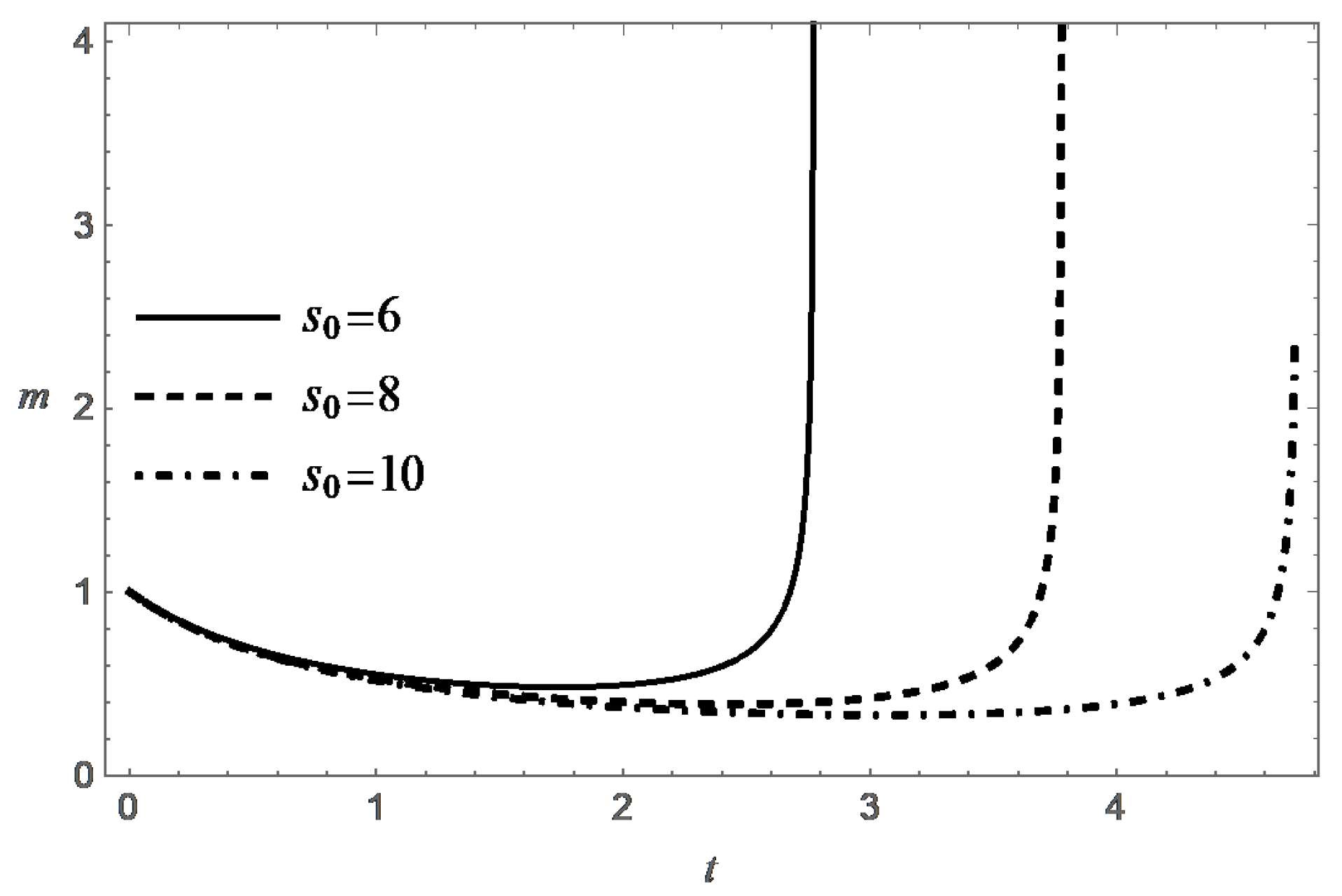
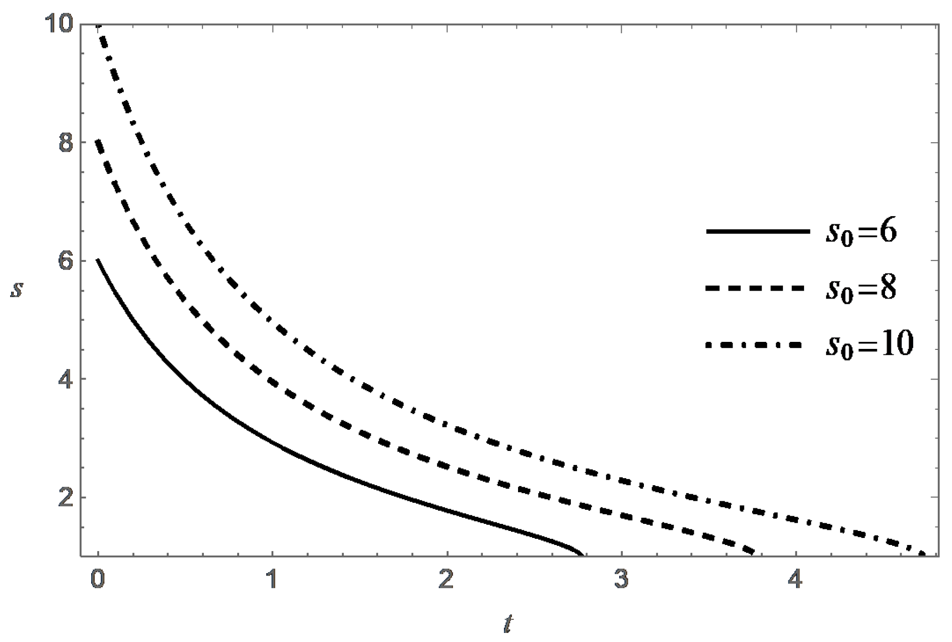
Remark 1.

If the value of $s_0-1>0$ is sufficiently small, then it is possible not only to make more precise the estimate of the lifetime $t^{*}$ of the solution of the problem (17), (18) in case (B), but also to obtain an asymptotically exact expression for this value at $s_0\to 1$:

$$t^{*}=\frac{2(s_0-1)}{3(m_0+\chi )}+O\left({(s_0-1)}^{3/2}\right).$$

Behavior of the functions m and s in the case (B) are presented in Figure 7, Figure 8, Figure 9, Figure 10, Figure 11 and Figure 12 for different values of $\chi$, $m_0$ and $s_0$.

Figure 7. The function m obtained by numerically solving the Cauchy problem (17) and (18) in case (B), where $m_0=1$, $s_0=2$ and for various values of $\chi$.

Figure 8. The function s obtained by numerically solving the Cauchy problem (17) and (18) in case (B), where $m_0=1$, $s_0=2$ and for various values of $\chi$.

Figure 9. The function m obtained by numerically solving the Cauchy problem (17) and (18) in case (B), where $\chi =1$, $s_0=4$ and for various values of $m_0$.

Figure 10. The function s obtained by numerically solving the Cauchy problem (17) and (18) in case (B), where $\chi =1$, $s_0=4$ and for various values of $m_0$.

Figure 11. The function m obtained by numerically solving the Cauchy problem (17) and (18) in case (B), where $\chi =1$, $m_0=1$ and for various values of $s_0$.

Figure 12. The function s obtained by numerically solving the Cauchy problem (17) and (18) in case (B), where $\chi =1$, $m_0=1$ and for various values of $s_0$.

3. On Partially Invariant Solutions

This section considers two classes of partially invariant solutions of Equation (2).

3.1. Constant $p_x$

For constant $p_x$ Equations (2) admit the generators

$${\partial }_t,{\partial }_y,x{\partial }_x+u{\partial }_u.$$

(25)

These generators are also admitted by the classical boundary layer equations [14]. In [24] these generators were exploited for finding a partially invariant solution of the classical boundary layer equations with the representation:

$$v=f\left(\tilde{u}\right),\tilde{u}=\frac{u}{x},$$

(26)

where a solution was obtained with $f=k\tilde{u}+k_1$.

Assume that $p_x=q$ is constant, and consider the partially invariant solution of system (2) with the representation:

$$v=k\tilde{u}+k_1.$$

Because of the Galilean transformation, one can assume that $k_1=0$. Substituting (26) into Equation (2), they become

$$x{\tilde{u}}_x+k{\tilde{u}}_y=-\tilde{u},$$

(27)

$$x{\tilde{u}}_{tyy}=x({\tilde{u}}_t-\chi {\tilde{u}}_{yy})+q.$$

(28)

The general solution of (27) is:

$$\tilde{u}(t,x,y)=\frac{1}{x}\psi (z,t),z=x^k{e}^{-y},$$

where $\psi (z,t)$ is an arbitrary function.

Substituting the latter into (28), it becomes:

$$z^2{\psi }_{tzz}+z{\psi }_{tz}+\chi (z^2{\psi }_{zz}+z{\psi }_z)={\psi }_t+q.$$

(29)

The latter equation is a linear equation. Assuming that:

$$\psi (z,t)=h_0\left(t\right)+\sum _{j=2}^m{h}_j\left(t\right)z^j,$$

where m is an arbitrary natural number; one finds that:

$$h_0=-qt+q_0,h_j=q_j{e}^{-\chi j^{2}t/(j^2-1)},(j\ge 2).$$

(30)

Suppose that

$$\psi (s,0)=q_0+\sum _{j=2}^{\infty }{q}_j{s}^j$$

(31)

is such that ${lim}_{j\to \infty }\frac{|q_{j+1}|}{|q_j|}=L>0$. Hence,

$$\underset{j\to \infty }{lim}\frac{|h_{j+1}|}{|h_j|}=L,$$

and the ratio test shows that the series

$$\psi (s,t)=h_0\left(t\right)+\sum _{j=2}^{\infty }{h}_j\left(t\right)s^j$$

(32)

converges with radius of convergence $r=L$. Due to the linearity of Equation (29), the function (32) is a solution of (29).

Remark 2.

Equation (29) can be reduced to an equation with constant coefficients. In fact, using the change:

$$\psi (z,t)=g(lnz,t),\lambda =lnz=klnx-y,$$

Equation (29) reduces to the equation:

$$g_{t\lambda \lambda }+\chi g_{\lambda \lambda }=g_t.$$

(33)

Due to equivalence transformations [13], we can consider, without loss of generality, that $q=0$. Using the method of separation of variables, assume that:

$$g(\lambda ,t)=h\left(t\right)\mu \left(\lambda \right).$$

Substituting this representation into (33), one obtains:

$$(h^{\prime }+\chi h){\mu }^{″}=h^{\prime }\mu .$$

Hence, for ${\mu }^{″}{h}^{\prime }\ne 0$ one gets:

$$\frac{\chi h}{h^{\prime }}+1=\frac{\mu }{{\mu }^{″}}=q_1,$$

where $q_1$ is constant such that $q_1(q_1-1)\ne 0$. The latter gives that:

$$h^{\prime }+\frac{\chi }{1-q_1}h=0,{\mu }^{″}-\frac{1}{q_1}\mu =0.$$

Hence, $h=e^{\chi t/(q_1-1)}$, and

$$\begin{array}{c}\mu =C_{1}sin\left(k_0\lambda \right)+C_{2}cos\left(k_0\lambda \right)\mathrm{for}{q}_1<0,k_0=\sqrt{-q_1^{-1}};\\ \mu =C_1{e}^{k_0\lambda }+C_2{e}^{-k_0\lambda }\mathrm{for}{q}_1>0,k_0=\sqrt{q_1^{-1}},\end{array}$$

where $C_1$ and $C_2$ are constant.

Because of linearity of Equation (33) these types of solutions also allow to obtain solutions in the form of series.

3.2. Case $p_x=e^{kt}F\left(x{e}^{-kt}\right)$

Consider a solution partially invariant with respect to the Lie algebra:

$${\partial }_y,{\partial }_t+k(x{\partial }_x+u{\partial }_u),$$

(34)

where $k\ne 0$ is constant. This Lie algebra is admitted by Equation (2) if $P(x,t)=e^{kt}F\left(x{e}^{-kt}\right)$. Invariants of this Lie algebra are:

$$v,x^{-1}u,x{e}^{-kt}.$$

The representation of the partially invariant solution has the form $v=f(\tilde{u},z)$, where $\tilde{u}=x^{-1}u$ and $z=x{e}^{-kt}$. Assume that $f(\tilde{u},z)=g_1\left(z\right)\tilde{u}+g_2\left(z\right)$. Using the change of variables from $(x,y,t)$ to $(y,z,t)$, and substituting the representation of the partially invariant solution into the second equation of (2), it becomes:

$$z{\tilde{u}}_z+g_1{\tilde{u}}_y=-\tilde{u}.$$

(35)

The general solution of (35) is:

$$\tilde{u}(t,y,z)=\frac{1}{z}\psi (s,t),s=e^{-y}g\left(z\right),$$

where $g_1\left(z\right)=z{g}^{\prime }\left(z\right)$, and $\psi (s,t)$ is an arbitrary function. The first equation of (2) reduces to the equation:

$$(kz{g}^{\prime }+g_2){\left(s^3{\psi }_{ss}\right)}_s-s{\left(s{\psi }_{ts}\right)}_s+{\psi }_t-(k+\chi )s{\left(s{\psi }_s\right)}_s+k\psi +F=0.$$

(36)

Differentiating the latter equation with respect to z, one obtains:

$$F^{\prime }=-{(kz{g}^{\prime }+g_2)}^{\prime }{\left(s^3{\psi }_{ss}\right)}_s,$$

(37)

and differentiating once more with respect to s, one derives that:

$${(kz{g}^{\prime }+g_2)}^{\prime }{\left(s^3{\psi }_{ss}\right)}_{ss}=0.$$

The case ${\left(s^3{\psi }_{ss}\right)}_{ss}=0$ leads to the trivial solution, hence, assume that:

$$kz{g}^{\prime }+g_2=k_1,$$

where $k_1$ is constant. Then F is constant, say $F=q$, and Equation (36) becomes:

$$k_1{\left(s^3{\psi }_{ss}\right)}_s-s{\left(s{\psi }_{ts}\right)}_s+{\psi }_t-(k+\chi )s{\left(s{\psi }_s\right)}_s+k\psi +q=0.$$

(38)

Equation (38) has solutions of the polynomial form:

$$\psi (s,t)=h_0\left(t\right)+\sum _{j=2}^m{h}_j\left(t\right)s^j,$$

(39)

where

$$h_0=-k^{-1}+q_0{e}^{-kt},h_j=q_j{e}^{-t(k-j{k}_1+\chi j^2/(j^2-1))},(j\ge 2),$$

(40)

m is arbitrary, and $q_j$ are constant. Notice that:

$$\frac{h_{j+1}}{h_j}=e^{t{k}_1}\frac{q_{j+1}}{q_j}{e}^{t\frac{\chi (2j+1)}{j(j^2-1)(j+2)}}.$$

Consider the function:

$$\psi (s,0)=q_0+\sum _{j=2}^{\infty }{q}_j{s}^j,$$

(41)

such that ${lim}_{j\to \infty }\frac{|q_{j+1}|}{|q_j|}=L>0$. Hence,

$$\underset{j\to \infty }{lim}\frac{|h_{j+1}|}{|h_j|}=e^{t{k}_1}L,$$

and the ratio test shows that the series

$$\psi (s,t)=h_0\left(t\right)+\sum _{j=2}^{\infty }{h}_j\left(t\right)s^j$$

(42)

converges with the radius of convergence $r=e^{t{k}_1}L$. Because of the linearity of the equation, the function (42) defines a solution of (38). Notice that for $k_1<0$ the radius of convergence decreases with increasing t.

Remark 3.

As the Lie algebra (34) is a subalgebra of the Lie algebra (25), then a similar form of a solution can be considered as in the previous case.

Remark 4.

Equation (38) can also be reduced to the linear equation with constant coefficients:

$$k_1{g}_{\lambda \lambda \lambda }-g_{\lambda \lambda t}-(k+\chi )g_{\lambda \lambda }-k_1{g}_{\lambda }+g_t+kg+q=0.$$

4. Boundary Layer near a Logarithmic Curve

The equations of a plane stationary boundary layer in a polymer solution near a solid rectilinear wall have the form:

$$u{(u-u_{yy})}_x+v{(u-u_{yy})}_y=-p_x+\chi u_{yy},u_x+v_y=0,$$

(43)

where $p\left(x\right)$ is a given function. Assume that $p\left(x\right)=-x^2/2$. Then system (43) admits the generators $x{\partial }_x+u{\partial }_u,{\partial }_y$, and hence their linear combination:

$$X=x{\partial }_x+u{\partial }_u-a{\partial }_y,$$

(44)

where a is constant. An invariant solution of system (44) with respect to generator (44) has the form:

$$u=xf\left(\zeta \right),v=g\left(\zeta \right),$$

(45)

where $\zeta =y+alnx$. The functions $f\left(\zeta \right)$ and $g\left(\zeta \right)$ satisfy the system of equations:

$$f\left(f-f^{″}+a(f^{\prime }-f^{‴})\right)+g(f^{\prime }-f^{‴})=1+\chi f^{″},f+a{f}^{\prime }+g^{\prime }=0,$$

(46)

where the prime denotes differentiation with respect to $\zeta$. Introducing a new unknown function $h=af+g$, then, due to the second equation in (46), the equality $f+h^{\prime }=0$ is true. From here and from the first equation in (46), the following equation for the function $h\left(\zeta \right)$ is obtained:

$$h{h}^{\left(iv\right)}-h^{\prime }{h}^{‴}-h{h}^{″}+{h^{\prime }}^2+\chi h^{‴}-1=0.$$

(47)

It is remarkable that Equation (47) does not contain the parameter a.

It is further assumed that $a>0$. We would like to describe on the basis of solution (45) the solution of the boundary layer problem near the curve $y=-alnx,x\ge 1$. For this, it is necessary to derive the equations of the boundary layer in a polymer solution on a curved boundary. In the classical theory of the boundary layer, curvilinear Misers coordinates are introduced for this [25,26]. As the new variable x, the length of the arc of the streamlined contour, measured from the initial point on it, is chosen, and the distance from the contour with the x coordinate along the normal to it is chosen for the new variable y. In the new variables, the equations of the plane boundary layer coincide with the original Prandtl equations. If we introduce the Misers variables into the initial equations of motion of the polymer solution in the Pavlovskii model, and perform their asymptotic simplification in the sense of the boundary layer theory, then at the limit for a stationary flow we obtain exactly Equation (43). The relation between the variable x in the obtained equations and the Cartesian coordinate $\overline{x}$ is given by the formula:

$$x=\sqrt{{\overline{x}}^2+a^2}-\sqrt{a}ln\frac{2a+2\sqrt{a({\overline{x}}^2+a^2)}}{\overline{x}},\overline{x}\ge 1.$$

(48)

It turns out that Equation (47) coincides with the notation with the equation arising in the analysis of the flow of a polymer solution near the stagnation point [18,19]. The corresponding boundary conditions for Equation (47) have the form:

$$h\left(0\right)=h^{\prime }\left(0\right)=0,h^{\prime }\to 1for\zeta \to \infty .$$

(49)

Defining the function $g\left(\zeta \right)$ by the relation $g=h+a{h}^{\prime }$, the second equation of (46) is satisfied and, in addition, by virtue of (48), the equality $g\left(0\right)=0$ holds. It follows from this and the equality $f=-h^{\prime }$ that the no-slip conditions $u=v=0$ are satisfied on the curve $y=-lnx$.

Remark 5.

Solution (45) of system (43) is defined for $x>0$. Notice that equations (43) admit the discrete symmetry $\tilde{x}=-x$, $\tilde{y}=y$, $\tilde{u}=-u$, $\tilde{v}=v$ and $\tilde{p}=p$. This allows us to extend solution (45) to negative values of x. In the domain $x<0$ the argument of the functions $f\left(\zeta \right)$ and $g\left(\zeta \right)$ is replaced with $y+aln(-x)$. The next transformation, $\widehat{x}=x+1$ if $x>0$, and $\widehat{x}=-x+1$ if $x<0$, makes it possible to determine a solution of type (45) already for all values of $x\in R$. As a result, we obtain a solution of system (43), which describes the boundary layer near the curve defined by the equations $y=-aln(x+1)$ for $x\ge 0$, and $y=-aln(-x+1)$ for $x\le 0$. At the origin, this curve has an angle point. In the classical boundary layer theory, it is well known the Falkner-Skan solution, which describes the boundary layer near a wedge ([27], see also [17]). This solution is self-similar. The solution we have obtained is not such, but it also has a group-theoretical nature.

5. Conclusions

The present paper deals with the plane unsteady boundary layer equations describing the behaviour of an aqueous polymer solution. These boundary layer equations for the Pavlovskii model and the Rivlin–Ericksen model were derived in [13], where a group analysis of these equations was performed. The present paper is devoted to constructing exact solutions of system (2), which is based on the Pavlovskii model. One of the problems considered in our paper is the problem of a flow of polymer solution near a stagnation point. We have found three exact solutions describing unsteady motion near the critical point, which differ in the form of conditions at infinity. The first solution (6) and (7), which satisfies the no-slip condition at $y=0$ and is bounded as $y\to \infty$, is derived by the method of differential constraints. The representations of the other two solutions (13) and (16) were obtained by noting that 1, $exp(y/s(t\left)\right)$ and $cos(y/s(t\left)\right)$ are elements of invariant subspaces of Equation (11). It should also be noted that Equation (11) was obtained as the reduced equation for a partially invariant solution [14] of the admitted Lie algebra (9). The main feature of these solutions is that they are reduced to solving ordinary differential equations. Another class of partially invariant solutions of system (2) was derived in Section 4. This class of partially invariant solutions contains two arbitrary functions. Equations of the boundary layer adjacent to the curvilinear boundary are formulated, and an invariant solution of the stationary problem in which the solid boundary is a logarithmic curve is constructed in Section 4.

The present paper is just the beginning of finding exact solutions of the boundary layer equations describing the behaviour of an aqueous polymer solution. Boundary layers in the model of second-grade fluid [27,28] and non-stationary boundary layers in the hereditary model (see [3] and references therein) have not been practically investigated. This area of fluid dynamics calls for further development.

References

- Pavlovskii, V.A. Theoretical description of weak aqueous polymer solutions. Dokl. Akad. Nauk SSSR 1971, 200, 809–812. [Google Scholar]
- Frolovskaya, O.A.; Pukhnachev, V.V. Analysis of the Models of Motion of Aqueous Solutions of Polymers on the Basis of Their Exact Solutions. Polymers 2018, 10, 684. [Google Scholar] [CrossRef] [PubMed] [Green Version]
- Amfilokhiev, V.B.; Pavlovskii, V.A.; Mazaeva, N.P.; Khodorkovskii, Y.S. Flows of polymer solutions in the presence of convective accelerations. Tr. Leningr. Korablestr. Inst. 1975, 96, 3–9. (In Russian) [Google Scholar]
- Oskolkov, A.P. On the uniqueness and global solvability of boundary-value problems for the equations of motion of aqueous solutions of polymers. Zap. Nauchn. Semin. LOMI 1973, 38, 98–136. (In Russian) [Google Scholar] [CrossRef]
- Oskolkov, A.P. Theory of nonstationary flows of Kelvin-Voigt fluids. J. Sov. Math. 1985, 28, 751–758. [Google Scholar] [CrossRef]
- Zvyagin, V.G.; Turbin, M.V. Mathematical Problems of the Dynamics of Viscoelastic Media; KRASAND: Moscow, Russia, 2012. (In Russian) [Google Scholar]
- Ladyzhenskaya, O.A. On the global unique solvability of some two-dimensional problems for the water solutions of polymers. J. Math. Sci. 2000, 99, 888–897. [Google Scholar] [CrossRef]
- Zvyagin, A.V. Investigation of the Solvability of a Stationary Motion of Weak Aqueous Polymer Solutions Model; Series Physics and Mathematics; Voronezh State University Bulletin: Voronezh, Russia, 2011; pp. 147–156. [Google Scholar]
- Baranovskii, E.S. Flows of a polymer fluid in domain with impermeable boundaries. Comput. Math. Math. Phys. 2014, 54, 1589–1596. [Google Scholar] [CrossRef]
- Bozhkov, Y.D.; Pukhnachev, V.V. Group analysis of equations of motion of aqueous solutions of polymers. Dokl. Phys. 2015, 60, 77–80. [Google Scholar] [CrossRef]
- Bozhkov, Y.D.; Pukhnachev, V.V.; Pukhnacheva, T.P. Mathematical models of polymer solutions motion and their symmetries. AIP Conf. Proc. 2015, 1684, 77–80. [Google Scholar] [CrossRef]
- Pukhnachev, V.V.; Frolovskaya, O.A. On the Voitkunskii-Amfilokhiev-Pavlovskii model of motion of aqueous polymer solutions. Proc. Steklov Inst. Math. 2018, 300, 168–181. [Google Scholar] [CrossRef]
- Meleshko, S.V.; Pukhnachev, V.V. Group analysis of boundary layer equations in the models of polymer solutions. Symmetry 2020, 12, 1084. [Google Scholar] [CrossRef]
- Ovsiannikov, L.V. Group Analysis of Differential Equations; Ames, W.F., Ed.; Academic Press: New York, NY, USA, 1982. [Google Scholar]
- Olver, P.J. Applications of Lie Groups to Differential Equations; Springer: New York, NY, USA, 1986. [Google Scholar]
- Hiemenz, K. Die Grenzschicht an einem in den gleichförmigen Flüssigkeitsstrom eingetauchten geraden Kreiszylinder. Dinglers Polytech. J. 1911, 326, 321–324. [Google Scholar]
- Schlichting, H.; Gersten, K. Boundary-Layer Theory, 8th ed.; Springer: Berlin/Heidelberg, Germany, 2000. [Google Scholar]
- Petrova, A.G. On the unique solvability of the problem of the flow of an aqueous solution of polymers near a critical point. Math. Notes 2019, 106, 784. [Google Scholar] [CrossRef]
- Petrova, A.G.; Pukhnachev, V.V.; Frolovskaya, O.A. Analytical and numerical investigation of unsteady flow near a critical point. Appl. Math. Mech. 2000, 80, 215–224. [Google Scholar] [CrossRef]
- Pukhnachev, V.V.; Frolovskaya, O.A.; Petrova, A.G. Solutions of polymers and their mathematical models. Bull. High. Educ. Institutions. North Cauc. Region. Nat. Sci. 2000, 2, 84–93. (In Russian) [Google Scholar]
- Sidorov, A.F.; Shapeev, V.P.; Yanenko, N.N. The Method of Differential Constraints and its Applications in Das Dynamics; Nauka: Novosibirsk, Russia, 1984. (In Russian) [Google Scholar]
- Meleshko, S.V. Methods for Constructing Exact Solutions of Partial Differential Equations; Mathematical and Analytical Techniques with Applications to Engineering; Springer: New York, NY, USA, 2005. [Google Scholar]
- Galaktionov, V.A.; Svirshchevskii, S.R. Exact Solutions and Invariant Subspaces of Nonlinear Partial Differential Equations in Mechanics and Physics; Chapman and Hall: Berlin, Germany, 2000. [Google Scholar]
- Ondich, J.R. A differential constraints approach to partial invariance. Eur. J. Appl. Math. 1995, 6, 631–637. [Google Scholar] [CrossRef]
- Mises, R. Bemerkungen zur Hydrodynamik. Zeitschr. Angew. Math. Mech. 1927, 7, 425–431. [Google Scholar]
- Kochin, N.E.; Kibel, I.A.; Rose, N.V. Theoretical Hydromechanics; John Wiley & Sons: New York, NY, USA, 1964; Part 2. [Google Scholar]
- Galdi, G.P.; Dalsen, M.G.V.; Sauer, N. Existence and uniqueness of classical solutions of equations of motion for second-grade fluids. Arch. Ration. Mech. Anal. 1993, 124, 221–237. [Google Scholar] [CrossRef]
- Roux, C.L. Existence and Uniqueness of the Flow of Second-Grade Fluids with Slip Boundary Conditions. Arch. Ration. Mech. Anal. 1999, 148, 309–356. [Google Scholar] [CrossRef]
Publisher’s Note: MDPI stays neutral with regard to jurisdictional claims in published maps and institutional affiliations. |
© 2021 by the authors. Licensee MDPI, Basel, Switzerland. This article is an open access article distributed under the terms and conditions of the Creative Commons Attribution (CC BY) license (https://creativecommons.org/licenses/by/4.0/).