Solvability Analysis of a Mixed Boundary Value Problem for Stationary Magnetohydrodynamic Equations of a Viscous Incompressible Fluid

Abstract

We investigate the boundary value problem for steady-state magnetohydrodynamic (MHD) equations with inhomogeneous mixed boundary conditions for a velocity vector, given the tangential component of a magnetic field. The problem represents the flow of electrically conducting viscous fluid in a 3D-bounded domain, which has the boundary comprising several parts with different physical properties. The global solvability of the boundary value problem is proved, a priori estimates of the solutions are obtained, and the sufficient conditions on data, which guarantee a solution’s local uniqueness, are determined.

1. Introduction. Statement of the Boundary Value Problem

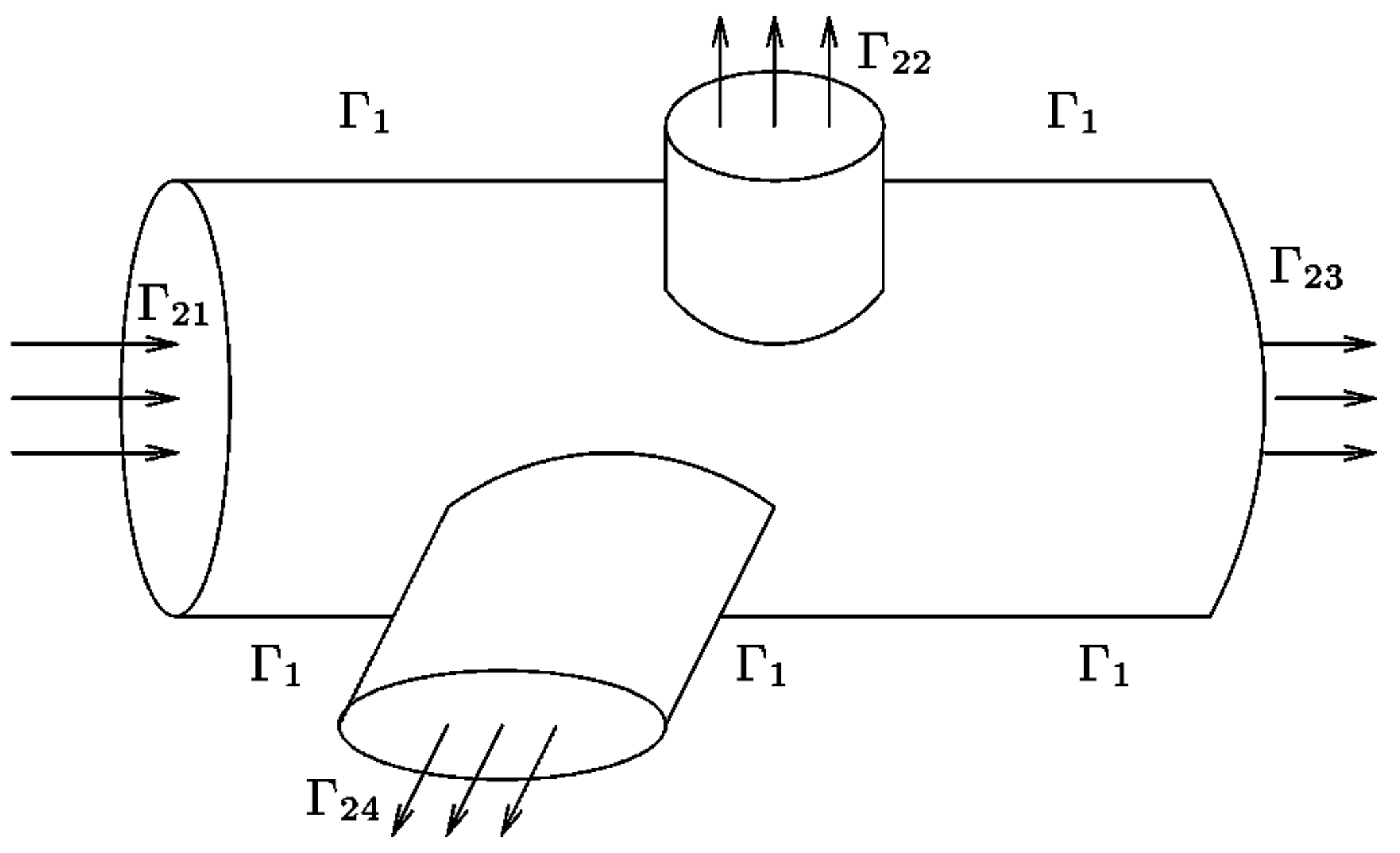
Let us assume that $\mathrm{\Omega }$ is a bounded domain from the space ${\mathrm{ℝ}}^3$ and it has the boundary $\mathrm{\Gamma }$, which includes three parts: ${\mathrm{\Gamma }}_1$, ${\mathrm{\Gamma }}_2$ and ${\mathrm{\Gamma }}_3$. We investigate the boundary value problem for the steady-state MHD equations with mixed boundary conditions for the velocity vector, given the magnetic field’s tangential component on the entire boundary:

$$\nu \mathrm{curl}\mathrm{curl}\mathbf{u}+\mathrm{curl}\mathbf{u}\times \mathbf{u}+\nabla r-\kappa \mathrm{curl}\mathbf{H}\times \mathbf{H}=\mathbf{f},\mathrm{div}\mathbf{u}=0\mathrm{in}\mathrm{\Omega },$$

(1)

$${\nu }_1\mathrm{curl}\mathbf{H}-\mathbf{E}+\kappa \mathbf{H}\times \mathbf{u}={\nu }_1\mathbf{j},\mathrm{div}\mathbf{H}=0,\mathrm{curl}\mathbf{E}=0\mathrm{in}\mathrm{\Omega },$$

(2)

$$\mathbf{u}=\mathbf{g}\mathrm{on}{\mathrm{\Gamma }}_1,\mathbf{u}\times \mathbf{n}=\mathbf{g}\times \mathbf{n}\mathrm{and}r=g\mathrm{on}{\mathrm{\Gamma }}_2,\mathrm{curl}\mathbf{u}\times \mathbf{n}=\mathbf{h},\mathbf{u}·\mathbf{n}=0\mathrm{on}{\mathrm{\Gamma }}_3,$$

(3)

$$\mathbf{H}\times \mathbf{n}=\mathbf{q}\mathrm{on}\mathrm{\Gamma }.$$

(4)

At this moment, $\mathbf{u}$ is a vector of velocity, and $\mathbf{H}$ is a magnetic field, $\mathbf{E}={\mathbf{E}}^{\prime }/{\rho }_0$, where ${\mathbf{E}}^{\prime }$ is an electric field. Here, $r=p+\frac{1}{2}{\left|\mathbf{u}\right|}^2$ is the total pressure, where $p=p^{\prime }/{\rho }_0$ and $p^{\prime }$ is the pressure; ${\rho }_0=\mathrm{const}$ is the fluid density; $\kappa =\mu /{\rho }_0$, ${\nu }_1=1/{\rho }_0\sigma =\kappa {\nu }_m$, $\nu$ and ${\nu }_m$ are the constant kinematic and magnetic viscosities; $\mu$ signifies the constant magnetic permeability; $\mathbf{j}$ means the current density; $\sigma$ is the constant conductivity; $\mathbf{n}$ is assigned for an outer normal to $\mathrm{\Gamma }$; and, finally, $\mathbf{f}$ is the volume density of external forces. Further, we will refer to the problem (1)–(4) with given functions $\mathbf{f},\mathbf{j},\mathbf{g},g$ and $\mathbf{q}$ as to Problem 1. We should pay attention that all the quantities in (1)–(4) are dimensional. Furthermore, their physical dimensions are defined exactly in terms of SI. Particularly, when $\mathbf{q}=\mathbf{0}$ in (4), it physically coincides with the situation that is often encountered in applications, where the boundary $\mathrm{\Gamma }$ is an ideal insulator.

By Figure 1, we illustrate an example, when a boundary $\mathrm{\Gamma }$ of a domain $\mathrm{\Omega }$ splits into two parts: ${\mathrm{\Gamma }}_1$ and ${\mathrm{\Gamma }}_2$. Furthermore, ${\mathrm{\Gamma }}_2={\mathrm{\Gamma }}_{21}\cup {\mathrm{\Gamma }}_{22}\cup {\mathrm{\Gamma }}_{23}\cup {\mathrm{\Gamma }}_{24}$.

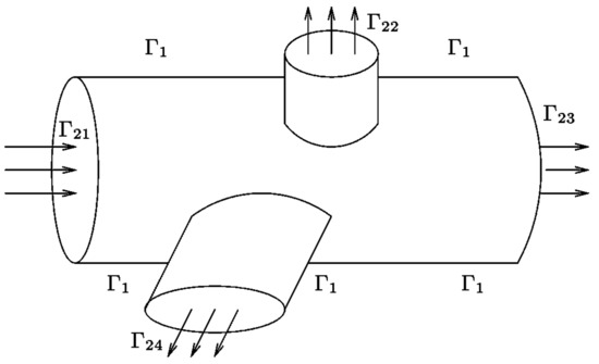
Figure 1. An example of the decomposition of the boundary into parts ${\mathrm{\Gamma }}_1$ and ${\mathrm{\Gamma }}_2$.

A sufficiently big amount of papers is devoted to the theoretical research of boundary value and control problems for the magnetic hydrodynamic Equations (1) and (2). In most papers, the MHD equations are examined under the Dirichlet boundary condition ${\mathbf{u}|}_{\mathrm{\Gamma }}=\mathbf{g}$ for the velocity vector, where $\mathbf{g}$ is a given function. Among these papers, we mention the articles [1,2,3,4,5,6] dedicated to the research of the solvability of the corresponding boundary value problems for Equations (1) and (2). Papers [7,8,9,10] are dedicated to the research of the solvability of both boundary value and control problems for (1) and (2). A number of papers are devoted to the investigation of the boundary value problems’ solvability for more general MHD models that take into account thermal effects (see, for example, [11,12,13]), effects that arise due to the presence of Hall currents [14], or effects caused by the micropolarity of a fluid [15].

In [16] the existence of a very weak solution of the boundary value problem for MHD equations with Dirichlet boundary condition for magnetic field is proved. In [17], a boundary value problem for steady-state MHD Equations (1) and (2) is studied in the case that zero tangential components of the velocity and magnetic field together with the total pressure are given on the entire boundary of the flow domain.

Substantially fewer works are about the investigation of Equations (1) and (2) with mixed boundary conditions of the type (3) for the velocity. The interest in boundary conditions of the form (3) is connected to the fact that in some physical situations, they are preferable to a standard Dirichlet condition for velocity (see, for more detail, [18,19,20]). The authors know only of Refs. [21,22], in which the solvability of the corresponding boundary value and control problems for equations of the form (1) and (2), or, for a more general magnetohydrodynamic model, taking into account thermal effects under the mixed boundary conditions for velocity, is proved. In particular, in [22], Equations (1) and (2) are studied under mixed boundary conditions (3) for the velocity vector, but under other ones for the electromagnetic field, compared to (4), which have the form $\mathbf{H}·\mathbf{n}=q$ and $\mathbf{E}\times \mathbf{n}=\mathbf{k}$ on $\mathrm{\Gamma }$, where q and $\mathbf{k}$ are functions given on the entire boundary $\mathrm{\Gamma }$. For the latest research on MHD models, one can refer to [23,24].

The purpose of this work, which continues the previous studies of the authors, is the theoretical analysis of Problem 1, which was formulated above. This analysis includes the study of global solvability of the mentioned boundary value problem and of sufficient conditions for the local uniqueness of its solution. Similar to the previous papers, the mathematical apparatus used by us is based on the application of the Schauder fixed point theorem and of lemmas of the velocity vector and magnetic field liftings.

Unlike earlier authors’ work [22], in this paper, we will look for the magnetic component $\mathbf{H}$ of the solution of Problem 1 in the subspace of the space $H^{s+1/2}{\left(\mathrm{\Omega }\right)}^3$, where $s\in [0,1/2]$. This subspace comprises solenoidal vector functions with a square-integrable rotor. The limiting case $s=0$ corresponds to the physical scenario, when the given magnetic field’s $\mathbf{H}$ tangential component $\mathbf{H}\times \mathbf{n}=\mathbf{q}$ on the boundary $\mathrm{\Gamma }$ is an element of the subspace of Hilbert space $L^2{\left(\mathrm{\Gamma }\right)}^3$. This scenario is the most preferable one from an applied point of view, especially while studying boundary control problems (see [10]).

Further, we will introduce an outline of the remainder of this paper. Firstly, in Section 2 the assumptions on the flow domain and its boundary are presented, the main function spaces and their norms and scalar products are described, and two auxiliary lemmas are formulated. In Section 3, the basic requirements on the initial data of Problem 1 are given, and its weak formulation is deduced. In Section 4, the two lemmas on the velocity vector and magnetic field liftings are formulated. Then, original Problem 1 is reduced with the help of mentioned lemmas to a homogeneous boundary value problem, and its solvability is proved by the Schauder fixed point theorem. The obtained result and the lifting lemmas imply the solvability of Problem 1. This main result of the paper is presented in the form of Theorem 1. Further, sufficient conditions providing local uniqueness of the solution to Problem 1 are established, which are presented in the form of Theorem 2. Section 5 contains the discussion of open problems and perspectives of applications of the obtained results while studying boundary control problems. The last Section 6 summarizes shortly our results and provides conclusive comments.

2. Functional Spaces and Assumptions

Let us presume that $\mathrm{\Omega }$ and the parts of its boundary ${\mathrm{\Gamma }}_1,{\mathrm{\Gamma }}_2$ and ${\mathrm{\Gamma }}_3$ fulfill as in [19] the following conditions:

(i) $\mathrm{\Omega }$ is a connected bounded domain in ${\mathrm{ℝ}}^3$, which has boundary $\mathrm{\Gamma }\in C^{1,1}$. Moreover, open parts ${\mathrm{\Gamma }}_1$, ${\mathrm{\Gamma }}_2$ and ${\mathrm{\Gamma }}_3$ of the boundary $\mathrm{\Gamma }$ fulfill the following conditions: ${\mathrm{\Gamma }}_1\ne \varnothing$, ${\mathrm{\Gamma }}_2\ne \varnothing$, ${\mathrm{\Gamma }}_i\cap {\mathrm{\Gamma }}_j=\varnothing$, $i\ne j$, ${\mathrm{\Gamma }}_j\in C^{1,1}$, $i,j=1,2,3$, $\mathrm{\Gamma }={\overline{\mathrm{\Gamma }}}_1\cup {\overline{\mathrm{\Gamma }}}_2\cup {\overline{\mathrm{\Gamma }}}_3$.

Additionally, we make use of the Sobolev functional spaces $H^s\left(D\right)$, where $s\in \mathrm{ℝ}$ and $L^{\mathrm{ℝ}}\left(D\right)$, $1\le \mathrm{ℝ}\le \infty$, where D can be either $\mathrm{\Omega }$ or $\mathrm{\Gamma }$ or a part of the boundary ${\mathrm{\Gamma }}_0$ of a positive measure. We designate the spaces of vector functions by $H^s{\left(D\right)}^3$ and $L^{\mathrm{ℝ}}{\left(\mathrm{\Omega }\right)}^3$. Moreover, the inner products in $L^2\left(\mathrm{\Omega }\right)$ and $L^2{\left(\mathrm{\Omega }\right)}^3$ are written down as $(·,·)$. Further, the inner products in $L^2\left(\mathrm{\Gamma }\right)$ or in $L^2\left({\mathrm{\Gamma }}_0\right)$ are introduced by ${(·,·)}_{\mathrm{\Gamma }}$ or ${(·,·)}_{{\mathrm{\Gamma }}_0}$. The norm in $L^2\left(\mathrm{\Omega }\right)$ or in $L^2\left({\mathrm{\Gamma }}_0\right)$ is given by ${\parallel ·\parallel }_{\mathrm{\Omega }}$ or ${\parallel ·\parallel }_{{\mathrm{\Gamma }}_0}$; the norm or seminorm in $H^1\left(\mathrm{\Omega }\right)$ and $H^1{\left(\mathrm{\Omega }\right)}^3$ is presented by ${\parallel ·\parallel }_{1,\mathrm{\Omega }}$ or ${|·|}_{1,\mathrm{\Omega }}$; and the norm in $H^s\left(\mathrm{\Gamma }\right)$ or $H^s\left({\mathrm{\Gamma }}_0\right)$ is denoted by ${\parallel ·\parallel }_{s,\mathrm{\Gamma }}$ or ${\parallel ·\parallel }_{s,{\mathrm{\Gamma }}_0}$. Finally, the duality for a pair X and $X^{*}$ is written as ${⟨·,·⟩}_{X^{*}\times X}$ or simply as $⟨·,·⟩$.

By $\mathcal{D}\left(\mathrm{\Omega }\right)$, it is denoted the space of infinitely differentiable functions, which have compact support in $\mathrm{\Omega }$ and let $H_0^1\left(\mathrm{\Omega }\right)$ signify the closure of $\mathcal{D}\left(\mathrm{\Omega }\right)$ in $H^1\left(\mathrm{\Omega }\right)$. Moreover, let the following hold:

$$H(\mathrm{curl};\mathrm{\Omega })=\{\mathbf{v}\in L^2{\left(\mathrm{\Omega }\right)}^3:\mathrm{curl}\mathbf{v}\in L^2{\left(\mathrm{\Omega }\right)}^3\},$$

$$H(\mathrm{div};\mathrm{\Omega })=\{\mathbf{v}\in L^2{\left(\mathrm{\Omega }\right)}^3:\mathrm{div}\mathbf{v}\in L^2\left(\mathrm{\Omega }\right)\},$$

$$H_{DC}\left(\mathrm{\Omega }\right)=H(\mathrm{curl};\mathrm{\Omega })\cap H(\mathrm{div};\mathrm{\Omega }).$$

where $H(\mathrm{curl};\mathrm{\Omega })$, $H(\mathrm{div};\mathrm{\Omega })$ and $H_{DC}\left(\mathrm{\Omega }\right)$ are Hilbert spaces regarding to the norms (see [25])

$${\parallel \mathbf{v}\parallel }_{\mathrm{curl},\mathrm{\Omega }}^2={\parallel \mathbf{v}\parallel }_{\mathrm{\Omega }}^2+{\parallel \mathrm{curl}\mathbf{v}\parallel }_{\mathrm{\Omega }}^2{,\parallel \mathbf{v}\parallel }_{\mathrm{div},\mathrm{\Omega }}^2={\parallel \mathbf{v}\parallel }_{\mathrm{\Omega }}^2+{\parallel \mathrm{div}\mathbf{v}\parallel }_{\mathrm{\Omega }}^2,$$

$${\parallel \mathbf{v}\parallel }_{H_{DC}\left(\mathrm{\Omega }\right)}^2={\parallel \mathbf{v}\parallel }_{\mathrm{\Omega }}^2+{\parallel \mathrm{curl}\mathbf{v}\parallel }_{\mathrm{\Omega }}^2+{\parallel \mathrm{div}\mathbf{v}\parallel }_{\mathrm{\Omega }}^2.$$

It is well known that under condition (i), there exist continuous linear trace operators $\gamma :H^1\left(\mathrm{\Omega }\right)\to H^{1/2}{\left(\mathrm{\Gamma }\right),\gamma |}_{{\mathrm{\Gamma }}_0}:H^1\left(\mathrm{\Omega }\right)\to H^{1/2}\left({\mathrm{\Gamma }}_0\right)$, where ${\mathrm{\Gamma }}_0$ is one of the parts ${\mathrm{\Gamma }}_1,{\mathrm{\Gamma }}_2$ and ${\mathrm{\Gamma }}_3$ of $\mathrm{\Gamma }$. To simplify the notation, we often write ${\phi |}_{\mathrm{\Gamma }}$, ${\phi |}_{{\mathrm{\Gamma }}_0}$ or ${\mathbf{u}|}_{\mathrm{\Gamma }}$, ${\mathbf{u}|}_{{\mathrm{\Gamma }}_0}$ instead of $\gamma \phi$, ${\gamma |}_{{\mathrm{\Gamma }}_0}\phi$ or $\gamma \mathbf{u}$, ${\gamma |}_{{\mathrm{\Gamma }}_0}\mathbf{u}$, if it does not create confusion.

Alongside the spaces $H^1{\left(\mathrm{\Omega }\right)}^3$, $L^2{\left(\mathrm{\Gamma }\right)}^3$, $H^{1/2}{\left(\mathrm{\Gamma }\right)}^3$ we consider their subspaces $H_T^1\left(\mathrm{\Omega }\right)$, $L_T^2\left(\mathrm{\Gamma }\right)$ and $H_T^{1/2}\left(\mathrm{\Gamma }\right)$, consisting of vectors tangential on $\mathrm{\Gamma }$ with norms, induced from $H^1{\left(\mathrm{\Omega }\right)}^3$, $L^2{\left(\mathrm{\Gamma }\right)}^3$ and $H^{1/2}{\left(\mathrm{\Gamma }\right)}^3$, and also the spaces $H^{-1}{\left(\mathrm{\Omega }\right)}^3$, $H_T^{-1}\left(\mathrm{\Omega }\right)$, $H^{-1/2}{\left(\mathrm{\Gamma }\right)}^3$ and $H_T^{-1/2}\left(\mathrm{\Gamma }\right)$, which are dual to $H_0^1{\left(\mathrm{\Omega }\right)}^3$, $H_T^1\left(\mathrm{\Omega }\right)$, $H^{1/2}{\left(\mathrm{\Gamma }\right)}^3$ and $H_T^{1/2}\left(\mathrm{\Gamma }\right)$ regarding to the spaces $L^2{\left(\mathrm{\Omega }\right)}^3$, $L^2{\left(\mathrm{\Omega }\right)}^3$, $L^2{\left(\mathrm{\Gamma }\right)}^3$ and $L_T^2\left(\mathrm{\Gamma }\right)$, respectively.

Below, we make use of the Green formulae [25]:

$$(\mathbf{u},\mathrm{grad}\phi )+(\mathrm{div}\mathbf{u},\phi )={⟨{\gamma }_n\mathbf{u},\phi ⟩}_{\mathrm{\Gamma }}\equiv {⟨\mathbf{u}·\mathbf{n},\phi ⟩}_{\mathrm{\Gamma }}\forall \mathbf{u}\in H(\mathrm{div};\mathrm{\Omega }),\phi \in H^1\left(\mathrm{\Omega }\right),$$

(5)

$$(\mathbf{q},\mathrm{curl}\mathbf{w})-(\mathrm{curl}\mathbf{q},\mathbf{w})={⟨{\gamma }_{\tau }\mathbf{q},{\mathbf{w}}_T⟩}_{\mathrm{\Gamma }}\equiv {⟨\mathbf{q}\times \mathbf{n},{\mathbf{w}}_T⟩}_{\mathrm{\Gamma }}$$

$$\forall \mathbf{q}\in H(\mathrm{curl};\mathrm{\Omega }),\mathbf{w}\in H^1{\left(\mathrm{\Omega }\right)}^3.$$

(6)

Here, ${\gamma }_n:H(\mathrm{div};\mathrm{\Omega })\to H^{-1/2}\left(\mathrm{\Gamma }\right)$ is a normal trace operator and ${\gamma }_{\tau }:H(\mathrm{curl};\mathrm{\Omega })\to H^{-1/2}{\left(\mathrm{\Gamma }\right)}^3$ is a tangential one.

Now, we introduce one more condition on the domain $\mathrm{\Omega }$ and on boundary $\mathrm{\Gamma }$:

(ii) $\mathrm{\Omega }$ is a bounded and finitely connected domain in ${\mathrm{ℝ}}^3$, and its boundary $\mathrm{\Gamma }\in C^{0,1}$ comprises $p_0+1$ connected components ${\mathrm{\Gamma }}_0,{\mathrm{\Gamma }}_1,\dots ,{\mathrm{\Gamma }}_{p_0}$. Here, ${\mathrm{\Gamma }}_0$ is a boundary of the unbounded component of the set ${\mathrm{ℝ}}^3\setminus \overline{\mathrm{\Omega }}$ and there exist the following surfaces ${\Sigma }_i\in C^2$, $i=1,2,\dots ,q_0$ such that ${\Sigma }_i\cap {\Sigma }_j=\varnothing$ for $i\ne j$ and set $\tilde{\mathrm{\Omega }}=\mathrm{\Omega }\setminus {\bigcup }_{i=1}^{q_0}{\Sigma }_i$ is simply connected and Lipschitz.

Note that the numbers $q_0$ and $p_0$, including those in condition (ii), are topological characteristics of the domain $\mathrm{\Omega }$. They are named first and second Betti numbers. Moreover, $p_0=0$ only in the case when the boundary $\mathrm{\Gamma }$ is connected. Stated differently, $\mathrm{\Gamma }={\mathrm{\Gamma }}_0$, and $q_0=0$ as long as $\mathrm{\Omega }$ is simply connected.

Let us introduce the next spaces:

$$\mathcal{H}\left(e\right)=\{\mathbf{h}\in L^2{\left(\mathrm{\Omega }\right)}^3:\mathrm{curl}\mathbf{h}=\mathbf{0},\mathrm{div}\mathbf{h}=0\mathrm{in}\mathrm{\Omega },\mathbf{h}\times \mathbf{n}=\mathbf{0}\mathrm{on}\mathrm{\Gamma }\},$$

$$\mathcal{H}\left(m\right)=\{\mathbf{h}\in L^2{\left(\mathrm{\Omega }\right)}^3:\mathrm{curl}\mathbf{h}=\mathbf{0},\mathrm{div}\mathbf{h}=0\mathrm{in}\mathrm{\Omega },\mathbf{h}·\mathbf{n}=0\mathrm{on}\mathrm{\Gamma }\},$$

$$X_N=\{\mathbf{h}\in H_{DC}\left(\mathrm{\Omega }\right):\mathbf{h}\times \mathbf{n}{|}_{\mathrm{\Gamma }}=\mathbf{0}\},$$

$$V_N=\{\mathbf{h}\in X_N\cap \mathcal{H}{\left(e\right)}^{\perp }:\mathrm{div}\mathbf{h}=0\}.$$

(7)

Here and below, $S^{\perp }$ denotes the orthogonal complement in $L^2{\left(\mathrm{\Omega }\right)}^3$ of an arbitrary subspace $S\subset L^2{\left(\mathrm{\Omega }\right)}^3$. The space $V_N$ specified in (7) will be used as the space of test functions for magnetic field. The spaces defined in (7) possess a number of important properties, which we present as the next lemma (see, for example, [26,27]).

Lemma 1.

Let the conditions (ii) be satisfied. Then:

(1) The spaces $\mathcal{H}\left(e\right)$ and $\mathcal{H}\left(m\right)$ are finitely dimensional and dim $\mathcal{H}\left(e\right)=p_0$, dim $\mathcal{H}\left(m\right)=q_0$, where the numbers $p_0$ and $q_0$ are defined in (ii);

(2) The following orthogonal decomposition holds:

$$L^2{\left(\mathrm{\Omega }\right)}^3=\mathrm{rot}{V}_N\oplus \nabla (H^1\left(\mathrm{\Omega }\right)\cap L_0^2\left(\mathrm{\Omega }\right))\oplus \mathcal{H}\left(m\right);$$

(8)

(3) The continuous embedding $X_N\subset H^1{\left(\mathrm{\Omega }\right)}^3$ takes place with equivalence between norms ${\parallel ·\parallel }_{DC}$ and ${\parallel ·\parallel }_{1,\mathrm{\Omega }}$ in the space $X_N$;

(4) There exists the constant ${\alpha }_1$ which depends on Ω such that the following holds:

$${\parallel \mathrm{curl}\mathbf{h}\parallel }_{\mathrm{\Omega }}^2\ge {\alpha }_1{\parallel \mathbf{h}\parallel }_{1,\mathrm{\Omega }}^2\forall \mathbf{h}\in V_N.$$

(9)

We remark that $\mathcal{H}\left(e\right)=\left\{0\right\}$, while presupposing that the boundary $\mathrm{\Gamma }$ is connected and $\mathcal{H}\left(m\right)=\left\{0\right\}$ when given that the domain $\mathrm{\Omega }$ is simply connected.

In addition to the general function spaces introduced above, we now define a number of special function spaces that will be essentially used below for deducing the weak formulation of Problem 1 and proving its solvability. We begin with defining the next boundary functional spaces:

$$H^{1/2}(\mathrm{\Gamma },\mathrm{\Gamma }\setminus {\mathrm{\Gamma }}_2)=\{\phi \in H^{1/2}\left(\mathrm{\Gamma }\right):\phi {|}_{\mathrm{\Gamma }\setminus {\mathrm{\Gamma }}_2}=0\},$$

$$H_0^{1/2}\left({\mathrm{\Gamma }}_2\right)=\{\phi {|}_{{\mathrm{\Gamma }}_2}:\phi \in H^{1/2}(\mathrm{\Gamma },\mathrm{\Gamma }\setminus {\mathrm{\Gamma }}_2)\},$$

$$H_T^{1/2}(\mathrm{\Gamma },\mathrm{\Gamma }\setminus {\mathrm{\Gamma }}_3)=\{\mathbf{v}\in H_T^{1/2}\left(\mathrm{\Gamma }\right):\mathbf{v}{|}_{\mathrm{\Gamma }\setminus {\mathrm{\Gamma }}_3}=\mathbf{0}\},$$

$$H_{T0}^{1/2}\left({\mathrm{\Gamma }}_3\right)=\{\mathbf{v}{|}_{{\mathrm{\Gamma }}_3}:\mathbf{v}\in H_T^{1/2}(\mathrm{\Gamma },\mathrm{\Gamma }\setminus {\mathrm{\Gamma }}_3)\}.$$

Together with the aforementioned spaces $H^{1/2}\left(\mathrm{\Gamma }\right)$, $H_0^{1/2}\left({\mathrm{\Gamma }}_2\right)$ and $H_{T,0}^{1/2}\left({\mathrm{\Gamma }}_3\right)$ their dual spaces $H^{-1/2}\left(\mathrm{\Gamma }\right)$, $H^{-1/2}\left({\mathrm{\Gamma }}_2\right)$ and $H_T^{-1/2}\left({\mathrm{\Gamma }}_3\right)$ are made use of. We present the duality relations in these spaces as ${⟨·,·⟩}_{\mathrm{\Gamma }}$, ${⟨·,·⟩}_{{\mathrm{\Gamma }}_2}$ and ${⟨·,·⟩}_{{\mathrm{\Gamma }}_3}$, respectively.

The following space is used as a space of test functions for the velocity vector $\mathbf{u}$:

$${\tilde{H}}_0^1{\left(\mathrm{\Omega }\right)}^3=\{\mathbf{v}\in H^1{\left(\mathrm{\Omega }\right)}^3{:\mathbf{v}|}_{{\mathrm{\Gamma }}_1}{=\mathbf{0},\mathbf{v}\times \mathbf{n}|}_{{\mathrm{\Gamma }}_2}=\mathbf{0},\mathbf{v}·\mathbf{n}{|}_{{\mathrm{\Gamma }}_3}=0\}.$$

Together with ${\tilde{H}}_0^1{\left(\mathrm{\Omega }\right)}^3$, we use its subspace

$$W=\{\mathbf{v}\in {\tilde{H}}_0^1{\left(\mathrm{\Omega }\right)}^3:\mathrm{div}\mathbf{v}=0\}$$

and also the space ${\tilde{H}}^{-1}{\left(\mathrm{\Omega }\right)}^3={\left({\tilde{H}}_0^1{\left(\mathrm{\Omega }\right)}^3\right)}^{*}$ dual of ${\tilde{H}}_0^1{\left(\mathrm{\Omega }\right)}^3$ with respect to $L^2{\left(\mathrm{\Omega }\right)}^3$ and the space $W^{*}$ dual of W.

When the vector $\mathbf{v}$ runs through the space ${\tilde{H}}_0^1{\left(\mathrm{\Omega }\right)}^3$, the restriction ${\mathbf{v}·\mathbf{n}|}_{{\mathrm{\Gamma }}_2}$ of its normal component on ${\mathrm{\Gamma }}_2$ ranges over the space $H_0^{1/2}\left({\mathrm{\Gamma }}_2\right)$, while the restriction ${\mathbf{v}}_T{|}_{{\mathrm{\Gamma }}_3}$ of its tangential component on ${\mathrm{\Gamma }}_3$ runs through the space $H_{T,0}^{1/2}\left({\mathrm{\Gamma }}_3\right)$. Moreover, the estimates hold (see [20]):

$${\parallel \mathbf{v}·\mathbf{n}\parallel }_{1/2,{\mathrm{\Gamma }}_2}\le C_{\mathrm{\Gamma }}^{\prime }{\parallel \mathbf{v}\parallel }_{1,\mathrm{\Omega }},\parallel {\mathbf{v}}_T{\parallel }_{1/2,{\mathrm{\Gamma }}_3}\le C_{\mathrm{\Gamma }}^{\prime \prime }{\parallel \mathbf{v}\parallel }_{1,\mathrm{\Omega }}\forall \mathbf{v}\in {\tilde{H}}_0^1{\left(\mathrm{\Omega }\right)}^3.$$

(10)

Here, $C_{\mathrm{\Gamma }}^{\prime }$ and $C_{\mathrm{\Gamma }}^{\prime \prime }$ are some constants, depending on $\mathrm{\Gamma }$.

Further, the following space plays a significant role:

$$H_T^{-1/2}({\mathrm{div}}_{\mathrm{\Gamma }};\mathrm{\Gamma })=\{\mathbf{w}\in H_T^{-1/2}\left(\mathrm{\Gamma }\right):{\mathrm{div}}_{\mathrm{\Gamma }}\mathbf{w}\in H^{-1/2}\left(\mathrm{\Gamma }\right)\},$$

equipped with the norm [26]

$${\parallel \mathbf{w}\parallel }_{-1/2,{\mathrm{div}}_{\mathrm{\Gamma }}}^2={\parallel \mathbf{w}\parallel }_{-1/2,\mathrm{\Gamma }}^2+{\parallel {\mathrm{div}}_{\mathrm{\Gamma }}\mathbf{w}\parallel }_{-1/2,\mathrm{\Gamma }}^2.$$

Here, ${\mathrm{div}}_{\mathrm{\Gamma }}$ is a linear operator of the surface divergence. It is well known (see [26]), that under condition $\mathrm{\Gamma }\in C^{1,1}$, the tangential trace operator ${\gamma }_{\tau }$ is a surjection of the space $H(\mathrm{curl},\mathrm{\Omega })$ onto the space $H_T^{-1/2}({\mathrm{div}}_{\mathrm{\Gamma }};\mathrm{\Gamma })$. Together with the space $H_T^{-1/2}({\mathrm{div}}_{\mathrm{\Gamma }};\mathrm{\Gamma })$, we use its subspace as follows:

$${\tilde{H}}_T^s\left(\mathrm{\Gamma }\right)=\{\mathbf{h}\in H_T^{-1/2}({\mathrm{div}}_{\mathrm{\Gamma }};\mathrm{\Gamma }):{\mathrm{div}}_{\mathrm{\Gamma }}\mathbf{h}=0,{\left(\mathbf{h},\mathbf{m}\right)}_{\mathrm{\Gamma }}=0\forall \mathbf{m}\in \mathcal{H}\left(m\right)\}\cap H_T^s\left(\mathrm{\Gamma }\right),s\ge 0$$

(11)

with the norm ${\parallel \mathbf{h}\parallel }_{{\tilde{H}}_T^s\left(\mathrm{\Gamma }\right)}={\parallel \mathbf{h}\parallel }_{s,\mathrm{\Gamma }}$ (see [10]). At $s=0$, we write ${\tilde{L}}_T^2\left(\mathrm{\Gamma }\right)$ instead of ${\tilde{H}}_T^s\left(\mathrm{\Gamma }\right)$.

Based on the spaces $H(\mathrm{curl},\mathrm{\Omega })$ and $H^{s+1/2}{\left(\mathrm{\Omega }\right)}^3$ we define their subspaces

$$H^0(\mathrm{curl},\mathrm{\Omega })=\{\mathbf{E}\in H(\mathrm{curl},\mathrm{\Omega }):\mathrm{curl}\mathbf{E}=\mathbf{0}\},$$

$${\mathcal{H}}_{\mathrm{div}}^{s+1/2}\left(\mathrm{\Omega }\right)=H^{s+1/2}{\left(\mathrm{\Omega }\right)}^3\cap \{\mathbf{H}\in H_{DC}\left(\mathrm{\Omega }\right):\mathrm{div}\mathbf{H}=0\}\cap \mathcal{H}{\left(e\right)}^{\perp },s\in [0,1/2],$$

(12)

equipped, respectively, with Hilbert norms as follows:

$${\parallel \mathbf{E}\parallel }_{H^0(\mathrm{curl},\mathrm{\Omega })}={\parallel \mathbf{E}\parallel }_{\mathrm{\Omega }}{,\parallel \mathbf{h}\parallel }_{{\mathcal{H}}_{\mathrm{div}}^{s+1/2}\left(\mathrm{\Omega }\right)}^2={\parallel \mathbf{h}\parallel }_{s,\mathrm{\Omega }}^2+{\parallel \mathrm{curl}\mathbf{h}\parallel }_{\mathrm{\Omega }}^2.$$

(13)

These spaces together with the space $H_T^1\left(\mathrm{\Omega }\right)$ play the main role in the sense that we are looking for the velocity $\mathbf{u}$ and also the magnetic $\mathbf{H}$ and the electrical $\mathbf{E}$ components of the solution $(\mathbf{u},\mathbf{H},\mathrm{ℝ},\mathbf{E})$ to Problem 1, respectively, exactly in the spaces $H_T^1\left(\mathrm{\Omega }\right)$, ${\mathcal{H}}_{\mathrm{div}}^{s+1/2}\left(\mathrm{\Omega }\right)$ and $H^0(\mathrm{curl},\mathrm{\Omega })$. As regards the total pressure r, this scalar component of the solution is sought in the space $L^2\left(\mathrm{\Omega }\right)$.

Finally, we define the following products of spaces:

$$H_{0N}={\tilde{H}}_0^1{\left(\mathrm{\Omega }\right)}^3\times V_N,V_{0N}=W\times V_N\subset H_{0N}$$

(14)

and their dual spaces $H_{0N}^{*}={\tilde{H}}^{-1}{\left(\mathrm{\Omega }\right)}^3\times V_N^{*}$ and $V_{0N}^{*}=W^{*}\times V_N^{*}$. $H_{0N}$ and $V_{0N}$ are Hilbert spaces provided with the norm as follows:

$${\parallel \left(\mathbf{u},\mathbf{H}\right)\parallel }_{H_{0N}}={\parallel \left(\mathbf{u},\mathbf{H}\right)\parallel }_{1,\mathrm{\Omega }}\equiv {(\parallel \mathbf{u}\parallel }_{1,\mathrm{\Omega }}^2+{\kappa \parallel \mathbf{H}\parallel }_{1,\mathrm{\Omega }}^2{)}^{1/2}.$$

(15)

The multiplier $\kappa$ in (15) serves, as in [9], to equalize the dimensions of each of terms in (15).

The elements of the dual space $H_{0N}^{*}$ (or $V_{0N}^{*}$) are the pairs $(\mathbf{f},\mathbf{l})\in {\tilde{H}}^{-1}{\left(\mathrm{\Omega }\right)}^3\times V_N^{*}$, (or $\left(\mathbf{f},\mathbf{l}\right)\in W^{*}\times V_N^{*}$) and, for example, the following:

$${⟨\left(\mathbf{f},\mathbf{l}\right),\left(\mathbf{v},\mathbf{\Psi }\right)⟩}_{H_{0N}^{*}\times H_{0N}}=$$

$$={⟨\mathbf{f},\mathbf{v}⟩}_{{\tilde{H}}^{-1}{\left(\mathrm{\Omega }\right)}^3\times {\tilde{H}}_0^1{\left(\mathrm{\Omega }\right)}^3}+{⟨\mathbf{l},\mathbf{\Psi }⟩}_{V_N^{*}\times V_N}\forall \left(\mathbf{v},\mathbf{\Psi }\right)\in H_{0N}.$$

Simple analysis shows that any element $\mathbf{f}\in {\tilde{H}}^{-1}{\left(\mathrm{\Omega }\right)}^3$ belongs to $W^{*}$, and any element $\mathbf{F}\equiv \left(\mathbf{f},\mathbf{l}\right)\in H_{0N}^{*}$ belongs to $V_{0N}^{*}$ and the following:

$${\parallel \mathbf{f}\parallel }_{W^{*}}\le {\parallel \mathbf{f}\parallel }_{{\tilde{H}}^{-1}{\left(\mathrm{\Omega }\right)}^3}{,\parallel \mathbf{F}\parallel }_{V_{0N}^{*}}\le {\parallel \mathbf{F}\parallel }_{H_{0N}^{*}}\le {\parallel \mathbf{f}\parallel }_{{\tilde{H}}^{-1}{\left(\mathrm{\Omega }\right)}^3}+{\kappa }^{-1/2}{\parallel \mathbf{l}\parallel }_{V_N^{*}}.$$

(16)

The products (14) serve as the spaces of test functions for main vector equations in (1) and (2) when deriving two equivalent weak formulations of Problem 1 in Section 3.

Below, while investigating the solvability of Problem 1, some properties of bilinear and trilinear forms which underlie the weak formulation of Problem 1 are used essentially. It is suitable for us to arrange these properties as the next lemma (see the details of the proof in [10,20,25,27]).

Lemma 2.

Under conditions (i) and (ii), there exist positive constants $C_0$, ${\alpha }_0$, β, ${\gamma }_0,{\gamma }_0^{\prime },{\gamma }_1,{\gamma }_2^{\prime }$ and ${\gamma }_2$, depending on Ω such that the following inequalities are fulfilled:

$$\left|(\mathrm{curl}\mathbf{u},\mathrm{curl}\mathbf{v})\right|\le C_0^2{\parallel \mathbf{u}\parallel }_{1,\mathrm{\Omega }}{\parallel \mathbf{v}\parallel }_{1,\mathrm{\Omega }}\forall \mathbf{u},\mathbf{v}\in H^1{\left(\mathrm{\Omega }\right)}^3,$$

(17)

$$(\mathrm{curl}\mathbf{v},\mathrm{curl}\mathbf{v})\ge {\alpha }_0{\parallel \mathbf{v}\parallel }_{1,\mathrm{\Omega }}^2\forall \mathbf{v}\in W,$$

(18)

$$\left|\left(\mathrm{curl}\mathbf{u}\times \mathbf{v},\mathbf{w}\right)\right|\le {\parallel \mathrm{curl}\mathbf{u}\parallel }_{\mathrm{\Omega }}{\parallel \mathbf{v}\parallel }_{L^4{\left(\mathrm{\Omega }\right)}^3}{\parallel \mathbf{w}\parallel }_{L^4{\left(\mathrm{\Omega }\right)}^3}\le$$

$$\le {\gamma }_0^{\prime }{\parallel \mathbf{u}\parallel }_{1,\mathrm{\Omega }}{\parallel \mathbf{v}\parallel }_{1,\mathrm{\Omega }}{\parallel \mathbf{w}\parallel }_{L^4{\left(\mathrm{\Omega }\right)}^3}\le {\gamma }_0{\parallel \mathbf{u}\parallel }_{1,\mathrm{\Omega }}{\parallel \mathbf{v}\parallel }_{1,\mathrm{\Omega }}{\parallel \mathbf{w}\parallel }_{1,\mathrm{\Omega }},$$

(19)

$$\left|\left(\mathrm{curl}\mathbf{u}\times \mathbf{v},\mathbf{w}\right)\right|\le {\gamma }_1{(\parallel \mathbf{u}\parallel }_{L^4{\left(\mathrm{\Omega }\right)}^3}+{\parallel \mathbf{u}|}_{\mathrm{\Gamma }}{\parallel }_{L^3{\left(\mathrm{\Gamma }\right)}^3}{)\parallel \mathbf{v}\parallel }_{1,\mathrm{\Omega }}{\parallel \mathbf{w}\parallel }_{1,\mathrm{\Omega }}\forall \mathbf{u},\mathbf{v},\mathbf{w}\in H^1{\left(\mathrm{\Omega }\right)}^3,$$

(20)

$$\left|\left(\mathrm{curl}\mathbf{\Psi }\times \mathbf{H},\mathbf{u}\right)\right|\le {\gamma }_2^{\prime }{\parallel \mathbf{H}\parallel }_{s+1/2,\mathrm{\Omega }}{\parallel \mathbf{u}\parallel }_{L^4{\left(\mathrm{\Omega }\right)}^3}{\parallel \mathbf{\Psi }\parallel }_{1,\mathrm{\Omega }}\le$$

$$\le {\gamma }_2{\parallel \mathbf{H}\parallel }_{s+1/2,\mathrm{\Omega }}{\parallel \mathbf{u}\parallel }_{1,\mathrm{\Omega }}{\parallel \mathbf{\Psi }\parallel }_{1,\mathrm{\Omega }}\forall \mathbf{u},\mathbf{\Psi }\in H^1{\left(\mathrm{\Omega }\right)}^3,\mathbf{H}\in H^{s+1/2}{\left(\mathrm{\Omega }\right)}^3,$$

(21)

$$|(\mathrm{curl}{\mathbf{H}}_1\times {\mathbf{H}}_2,\mathbf{u})|\le {\gamma }_2^{\prime }\parallel \mathrm{curl}{\mathbf{H}}_1{\parallel }_{\mathrm{\Omega }}\parallel {\mathbf{H}}_2{\parallel }_{s+1/2,\mathrm{\Omega }}{\parallel \mathbf{u}\parallel }_{L^4{\left(\mathrm{\Omega }\right)}^3}\le$$

$$\le {\gamma }_2\parallel \mathrm{curl}{\mathbf{H}}_1{\parallel }_{\mathrm{\Omega }}\parallel {\mathbf{H}}_2{\parallel }_{s+1/2,\mathrm{\Omega }}{\parallel \mathbf{u}\parallel }_{1,\mathrm{\Omega }}$$

$$\forall {\mathbf{H}}_1\in {\mathcal{H}}_{\mathrm{div}}^{s+1/2}\left(\mathrm{\Omega }\right),{\mathbf{H}}_2\in H^{s+1/2}{\left(\mathrm{\Omega }\right)}^3,\mathbf{u}\in H^1{\left(\mathrm{\Omega }\right)}^3,$$

(22)

where $s\in [0,1/2]$. Moreover, the inf-sup condition

$$\underset{\mathrm{ℝ}\in L^2\left(\mathrm{\Omega }\right)}{inf}\underset{\mathbf{v}\in {\tilde{H}}_0^1{\left(\mathrm{\Omega }\right)}^3}{sup}\frac{-(\mathrm{div}\mathbf{v},\mathrm{ℝ})}{{\parallel \mathbf{v}\parallel }_{1,\mathrm{\Omega }}{\parallel \mathrm{ℝ}\parallel }_{\mathrm{\Omega }}}\ge \beta$$

(23)

takes place, and the next relation is carried out as follows:

$$\left(\mathrm{curl}\mathbf{\Psi }\times \mathbf{H},\mathbf{u}\right)=(\mathbf{H}\times \mathbf{u},\mathrm{curl}\mathbf{\Psi })=-\left(\mathrm{curl}\mathbf{\Psi }\times \mathbf{u},\mathbf{H}\right)$$

$$\forall \mathbf{\Psi },\mathbf{u}\in H^1{\left(\mathrm{\Omega }\right)}^3,\mathbf{H}\in H^{s+1/2}{\left(\mathrm{\Omega }\right)}^3.$$

(24)

3. Weak Formulation of Problem 1. Weak Solution

Let, in addition to conditions (i) and (ii), the following conditions be fulfilled:

(iii) $\mathbf{f}\in {\tilde{H}}^{-1}{\left(\mathrm{\Omega }\right)}^3$, $\mathbf{j}\in L^2{\left(\mathrm{\Omega }\right)}^3$, $g\in H^{-1/2}\left({\mathrm{\Gamma }}_2\right)$, $\mathbf{h}\in H_T^{-1/2}\left({\mathrm{\Gamma }}_3\right)$,

(iv) $\mathbf{g}\in H_T^{1/2}\left(\mathrm{\Gamma }\right)$,

(v) $\mathbf{q}\in {\tilde{H}}_T^s\left(\mathrm{\Gamma }\right)$, $s\in [0,1/2]$.

We introduce the functionals

$$\tilde{\mathbf{f}}:{\tilde{H}}_0^1{\left(\mathrm{\Omega }\right)}^3\to \mathrm{ℝ},\mathbf{F}:{\tilde{H}}_0^1{\left(\mathrm{\Omega }\right)}^3\times V_N\to \mathrm{ℝ}$$

by the formulae

$$⟨\tilde{\mathbf{f}},\mathbf{v}⟩\equiv {⟨\tilde{\mathbf{f}},\mathbf{v}⟩}_{{\tilde{H}}^{-1}{\left(\mathrm{\Omega }\right)}^3\times {\tilde{H}}_0^1{\left(\mathrm{\Omega }\right)}^3}={⟨\mathbf{f},\mathbf{v}⟩}_{{\tilde{H}}^{-1}{\left(\mathrm{\Omega }\right)}^3\times {\tilde{H}}_0^1{\left(\mathrm{\Omega }\right)}^3}-{⟨g,\mathbf{v}·\mathbf{n}⟩}_{{\mathrm{\Gamma }}_2}+{⟨\mathbf{h},{\mathbf{v}}_T⟩}_{{\mathrm{\Gamma }}_3},$$

$$⟨\mathbf{F},\left(\mathbf{v},\mathbf{\Psi }\right)⟩=⟨\tilde{\mathbf{f}},\mathbf{v}⟩+{\nu }_1(\mathbf{j},\mathrm{rot}\mathbf{\Psi }).$$

(25)

From (10), (16) and (25), it follows by condition (iii) that $\tilde{\mathbf{f}}\in {\tilde{H}}^{-1}{\left(\mathrm{\Omega }\right)}^3$, $F\in H_{0N}^{*}$ and

$$\parallel \tilde{\mathbf{f}}{\parallel }_{{\tilde{H}}^{-1}{\left(\mathrm{\Omega }\right)}^3}\le {\parallel \mathbf{f}\parallel }_{{\tilde{H}}^{-1}{\left(\mathrm{\Omega }\right)}^3}+C_{\mathrm{\Gamma }}^{\prime }{\parallel g\parallel }_{-1/2,{\mathrm{\Gamma }}_2}+C_{\mathrm{\Gamma }}^{\prime \prime }{\parallel \mathbf{h}\parallel }_{-1/2,{\mathrm{\Gamma }}_3},{\parallel \mathbf{F}\parallel }_{H_{0N}^{*}}\le M.$$

Here, M is a constant defined by the following:

$$M={\parallel \mathbf{f}\parallel }_{{\tilde{H}}^{-1}{\left(\mathrm{\Omega }\right)}^3}+C_{\mathrm{\Gamma }}^{\prime }{\parallel g\parallel }_{-1/2,{\mathrm{\Gamma }}_2}+C_{\mathrm{\Gamma }}^{\prime \prime }{\parallel \mathbf{h}\parallel }_{-1/2,{\mathrm{\Gamma }}_3}+{\kappa }^{-1/2}{C}_0{\nu }_1{\parallel \mathbf{j}\parallel }_{\mathrm{\Omega }}.$$

(26)

Let us deduce a weak formulation of Problem 1. Suppose that the quadruple $(\mathbf{u},\mathbf{H},\mathrm{ℝ},\mathbf{E})\in C^2{\left(\overline{\mathrm{\Omega }}\right)}^3\times C^1{\left(\overline{\mathrm{\Omega }}\right)}^3\times C^1\left(\overline{\mathrm{\Omega }}\right)\times C^1{\left(\overline{\mathrm{\Omega }}\right)}^3$ is a classic solution to Problem 1. Firstly, we note that by conditions $\mathrm{curl}\mathbf{E}=\mathbf{0}$ and ${\mathbf{\Psi }\times \mathbf{n}|}_{\mathrm{\Gamma }}=\mathbf{0}$ for any $\mathbf{\Psi }\in V_N$ and by using Green Formula (6), we have the following:

$$(\mathbf{E},\mathrm{curl}\mathbf{\Psi })=(\mathrm{curl}\mathbf{E},\mathbf{\Psi })+{⟨\mathbf{\Psi }\times \mathbf{n},{\mathbf{E}}_T⟩}_{\mathrm{\Gamma }}=0\forall \mathbf{\Psi }\in V_N.$$

(27)

At this point, the first equation in (1) is multiplied by the function $\mathbf{v}\in {\tilde{H}}_0^1{\left(\mathrm{\Omega }\right)}^3$ and the first one in (2) by $\mathrm{curl}\mathbf{\Psi }$, $\mathbf{\Psi }\in V_N$. Further, the integration over $\mathrm{\Omega }$ is conducted alongside with applying Green’s formulas (5) and (6). After considering (27) and (25), we obtain the following:

$$\nu (\mathrm{curl}\mathbf{u},\mathrm{curl}\mathbf{v})+(\mathrm{curl}\mathbf{u}\times \mathbf{u},\mathbf{v})-(\mathrm{div}\mathbf{v},\mathrm{ℝ})-$$

$$-\kappa (\mathrm{curl}\mathbf{H}\times \mathbf{H},\mathbf{v})=⟨\tilde{\mathbf{f}},\mathbf{v}⟩\forall \mathbf{v}\in {\tilde{H}}_0^1{\left(\mathrm{\Omega }\right)}^3,$$

(28)

$${\nu }_1(\mathrm{curl}\mathbf{H},\mathrm{curl}\mathbf{\Psi })+\kappa (\mathrm{curl}\mathbf{\Psi }\times \mathbf{H},\mathbf{u})={\nu }_1(\mathbf{j},\mathrm{curl}\mathbf{\Psi })\forall \mathbf{\Psi }\in V_N.$$

(29)

By adding (28) and (29), we attain a special formulation of Problem 1, the solving of which is necessary to find a triple $(\mathbf{u},\mathbf{H},\mathrm{ℝ})\in H_T^1\left(\mathrm{\Omega }\right)\times {\mathcal{H}}_{\mathrm{div}}^{s+1/2}\left(\mathrm{\Omega }\right)\times L^2\left(\mathrm{\Omega }\right)$, satisfying the following relations:

$$\nu (\mathrm{curl}\mathbf{u},\mathrm{curl}\mathbf{v})+{\nu }_1(\mathrm{curl}\mathbf{H},\mathrm{curl}\mathbf{\Psi })-(\mathrm{div}\mathbf{v},\mathrm{ℝ})+\left(\mathrm{curl}\mathbf{u}\times \mathbf{u},\mathbf{v}\right)+$$

$$+\kappa [\left(\mathrm{curl}\mathbf{\Psi }\times \mathbf{H},\mathbf{u}\right)-\left(\mathrm{curl}\mathbf{H}\times \mathbf{H},\mathbf{v}\right)]=⟨\mathbf{F},\left(\mathbf{v},\mathbf{\Psi }\right)⟩\forall \left(\mathbf{v},\mathbf{\Psi }\right)\in H_{0N},$$

(30)

$$\mathrm{div}\mathbf{u}=0\mathrm{in}\mathrm{\Omega },\mathbf{u}=\mathbf{g}\mathrm{on}{\mathrm{\Gamma }}_1,\mathbf{u}\times \mathbf{n}=\mathbf{g}\times \mathbf{n}\mathrm{on}{\mathrm{\Gamma }}_2,\mathbf{u}·\mathbf{n}=0\mathrm{on}{\mathrm{\Gamma }}_3,$$

$$\mathbf{H}\times \mathbf{n}=\mathbf{q}\mathrm{on}\mathrm{\Gamma }.$$

(31)

Now, we study the properties of the solution of problem (30), (31) and show that (30) and (31) can be considered to be weak formulations of Problem 1. Let the triple $(\mathbf{u},\mathbf{H},\mathrm{ℝ})\in H_T^1\left(\mathrm{\Omega }\right)\times {\mathcal{H}}_{\mathrm{div}}^{s+1/2}\left(\mathrm{\Omega }\right)\times L^2\left(\mathrm{\Omega }\right)$ be a solution of problem (30), (31). Considering the restriction of (30) on the space $V_{0N}$, we infer that the pair $\left(\mathbf{u},\mathbf{H}\right)\in H_T^1\left(\mathrm{\Omega }\right)\times {\mathcal{H}}_{\mathrm{div}}^{s+1/2}\left(\mathrm{\Omega }\right)$ meets the following identity:

$$\nu (\mathrm{curl}\mathbf{u},\mathrm{curl}\mathbf{v})+{\nu }_1(\mathrm{curl}\mathbf{H},\mathrm{curl}\mathbf{\Psi })+\left(\mathrm{curl}\mathbf{u}\times \mathbf{u},\mathbf{v}\right)+$$

$$+\kappa \left(\mathrm{curl}\mathbf{\Psi }\times \mathbf{H},\mathbf{u}\right)-\kappa \left(\mathrm{curl}\mathbf{H}\times \mathbf{H},\mathbf{v}\right)=⟨\mathbf{F},\left(\mathbf{v},\mathbf{\Psi }\right)⟩\forall \left(\mathbf{v},\mathbf{\Psi }\right)\in V_{0N}.$$

(32)

It is significant to observe that though the identity (32) does not comprise the pair $(\mathrm{ℝ},\mathbf{E})$, the latter can be recovered from the pair $\left(\mathbf{u},\mathbf{H}\right)\in H_T^1\left(\mathrm{\Omega }\right)\times {\mathcal{H}}_{\mathrm{div}}^{s+1/2}\left(\mathrm{\Omega }\right)$ satisfying (32) so that the Equations (1) and (2) are fulfilled in a certain sense. Indeed, setting $\mathbf{v}=\mathbf{0}$ in (32), we arrive at identity (29), which can be rewritten in the following form:

$$({\nu }_1\mathrm{curl}\mathbf{H}+\kappa \mathbf{H}\times \mathbf{u}-{\nu }_1\mathbf{j},\mathrm{curl}\mathbf{\Psi })=0\forall \mathbf{\Psi }\in V_N.$$

(33)

The expression of (33) means that vector ${\nu }_1\mathrm{curl}\mathbf{H}+\kappa \mathbf{H}\times \mathbf{u}-{\nu }_1\mathbf{j}$ is orthogonal in $L^2{\left(\mathrm{\Omega }\right)}^3$ to vector $\mathrm{curl}\mathbf{\Psi }$ for any $\mathbf{\Psi }\in V_N$. It is possible by orthogonal decomposition (8) if and only if the following holds:

$${\nu }_1\mathrm{curl}\mathbf{H}+\kappa \mathbf{H}\times \mathbf{u}-{\nu }_1\mathbf{j}=\nabla \phi +\mathbf{m}a.e.\mathrm{in}\mathrm{\Omega }.$$

(34)

Here, $\phi \in H^1\left(\mathrm{\Omega }\right)\cap L_0^2\left(\mathrm{\Omega }\right)$ and $\mathbf{m}\in \mathcal{H}\left(m\right)$ are certain elements which are defined uniquely by the left-hand side of (34). Since $\mathrm{curl}\nabla \phi =\mathbf{0}$ and $\mathrm{curl}\mathbf{m}=\mathbf{0}$ in $\mathrm{\Omega }$, then setting $\mathbf{E}\equiv \nabla \phi +\mathbf{m}$, from (34), we infer that vector $\mathbf{E}$ appears to be an electrical component of the solution of Problem 1. This means the vector $\mathbf{E}$ fulfills $\mathrm{curl}\mathbf{E}=\mathbf{0}$ in $\mathrm{\Omega }$ while the triple $\left(\mathbf{u},\mathbf{H},\mathbf{E}\right)$ fulfills the first equation in (2) almost everywhere in $\mathrm{\Omega }$.

As for the recovery of component r from the identity (32), this procedure is performed using the inf-sup condition (23) according to the standard scheme using de Rham theory (see details, for example, in [25]). For convenience of readers we offer here a brief outline of this procedure following [4]. To this end, we represent a functional as follows:

$$\mathbf{L}=\mathbf{L}(\mathbf{u},\mathbf{H},\mathbf{f}):{\tilde{H}}_0^1{\left(\mathrm{\Omega }\right)}^3\to \mathrm{ℝ}$$

by

$$⟨\mathbf{L},\mathbf{v}⟩=\nu (\mathrm{curl}\mathbf{u},\mathrm{curl}\mathbf{v})+(\mathrm{curl}\mathbf{u}\times \mathbf{u},\mathbf{v})-\kappa \left(\mathrm{curl}\mathbf{H}\times \mathbf{H},\mathbf{v}\right)-⟨\mathbf{f},\mathbf{v}⟩.$$

From the identity (32), the properties of the pair $\left(\mathbf{u},\mathbf{H}\right)$ and from the condition $\mathbf{f}\in {\tilde{H}}^{-1}{\left(\mathrm{\Omega }\right)}^3$ it can be inferred that $\mathbf{L}\in {\tilde{H}}^{-1}{\left(\mathrm{\Omega }\right)}^3$ and

$$⟨\mathbf{L},\mathbf{v}⟩=0\forall \mathbf{v}\in W.$$

As the form $-(\mathrm{div}·,·)$ satisfies inf-sup condition (23) on ${\tilde{H}}_0^1{\left(\mathrm{\Omega }\right)}^3\times L^2\left(\mathrm{\Omega }\right)$, then there exists a unique function $\mathrm{ℝ}\in L^2\left(\mathrm{\Omega }\right)$ such that there holds identity (see [25])

$$⟨\mathbf{L},\mathbf{v}⟩=-⟨\mathrm{grad}\mathrm{ℝ},\mathbf{v}⟩=(\mathrm{div}\mathbf{v},\mathrm{ℝ})\forall \mathbf{v}\in {\tilde{H}}_0^1{\left(\mathrm{\Omega }\right)}^3$$

which coincides with (28). Adding (28) with (29) we obtain (30). Choosing $\mathbf{v}\in \mathcal{D}{\left(\mathrm{\Omega }\right)}^3\subset {\tilde{H}}_0^1{\left(\mathrm{\Omega }\right)}^3$ in (28), we obtain the following relation:

$$-\nu \mathrm{curl}\mathrm{curl}\mathbf{u}+\mathrm{curl}\mathbf{u}\times \mathbf{u}+\nabla \mathrm{ℝ}-\kappa \mathrm{curl}\mathbf{H}\times \mathbf{H}=\mathbf{f}\mathrm{in}{\left({\mathcal{D}}^{\prime }\left(\mathrm{\Omega }\right)\right)}^3.$$

(35)

It means that the first equation in (1) is fulfilled in a distribution sense.

The above results lead to the conclusion that as a weak formulation of Problem 1, one can choose both problem (30), (31) with respect to the triple $(\mathbf{u},\mathbf{H},\mathrm{ℝ})\in H_T^1\left(\mathrm{\Omega }\right)\times {\mathcal{H}}_{\mathrm{div}}^{s+1/2}\left(\mathrm{\Omega }\right)\times L^2\left(\mathrm{\Omega }\right)$ as well as problem (31), (32) for the pair $\left(\mathbf{u},\mathbf{H}\right)\in H_T^1\left(\mathrm{\Omega }\right)\times {\mathcal{H}}_{\mathrm{div}}^{s+1/2}\left(\mathrm{\Omega }\right)$. Based on the first option, we introduce the following important definition.

Definition 1.

Any triple $(\mathbf{u},\mathbf{H},\mathrm{ℝ})\in H_T^1\left(\mathrm{\Omega }\right)\times {\mathcal{H}}_{\mathrm{div}}^{s+1/2}\left(\mathrm{\Omega }\right)\times L^2\left(\mathrm{\Omega }\right)$ is called a weak solution of Problem 1 if it satisfies the relations (30) and (31).

For further analysis, it is convenient for us to organize the results of the prior analysis as the lemma, which greatly facilitates below the proof of the weak solvability of Problem 1.

Lemma 3.

Let conditions (i)–(v) hold and let $(\mathbf{u},\mathbf{H})\in H_T^1\left(\mathrm{\Omega }\right)\times {\mathcal{H}}_{\mathrm{div}}^{s+1/2}\left(\mathrm{\Omega }\right)$ be a solution to the problem (31), (32). In that case, there exist functions $\mathrm{ℝ}\in L^2\left(\mathrm{\Omega }\right)$ and $\mathbf{E}\in H^0(\mathrm{curl},\mathrm{\Omega })$ uniquely defined by the pair $\left(\mathbf{u},\mathbf{H}\right)$. As the triple $(\mathbf{u},\mathbf{H},\mathrm{ℝ})$ is a weak solution to Problem 1, while the quadruple $(\mathbf{u},\mathbf{H},\mathrm{ℝ},\mathbf{E})$ meets all boundary conditions in (3) and (4) in the sense of traces, Equation (2) a.e. in Ω and the first equation in (1) do so in the distribution sense (35).

Our further goal is to prove the existence of a weak solution to Problem 1 and to establish sufficient conditions providing the local uniqueness of the weak solution. The proof of the existence will be based on the reduction of the original inhomogeneous Problem 1 to an equivalent homogeneous boundary value problem, using the two special lemmas on velocity vector and magnetic field liftings (see below).

4. Solvability of Problem 1

Now, we are going to justify the existence of the weak solution of Problem 1. For this purpose, we reduce Problem 1 to the equivalent homogeneous boundary value problem using the following two lemmas on the existence of velocity vector and magnetic field liftings with prescribed properties. More detailed information about these lemmas can be discovered in [20,22,26].

Lemma 4.

Let, under the assumptions (i) and (ii), $\mathbf{g}\in H_T^{1/2}\left(\mathrm{\Gamma }\right)$. Then, for any number $\epsilon >0$, there exists ${\mathbf{u}}_{\epsilon }\in H_T^1\left(\mathrm{\Omega }\right)$ such that the following holds:

$$\mathrm{div}{\mathbf{u}}_{\epsilon }=0in\mathrm{\Omega },{\mathbf{u}}_{\epsilon }=\mathbf{g}on{\mathrm{\Gamma }}_1,{\mathbf{u}}_{\epsilon }\times \mathbf{n}=\mathbf{g}\times \mathbf{n}on{\mathrm{\Gamma }}_{2}and{\mathbf{u}}_{\epsilon }·\mathbf{n}=0on{\mathrm{\Gamma }}_3,$$

(36)

$$\parallel {\mathbf{u}}_{\epsilon }{\parallel }_{L^4{\left(\mathrm{\Omega }\right)}^3}\le \epsilon M_{\mathbf{g}},\parallel {\mathbf{u}}_{\epsilon }{\parallel }_{1,\mathrm{\Omega }}\le C_{\epsilon }{M}_{\mathbf{g}},M_{\mathbf{g}}={\parallel \mathbf{g}\parallel }_{1/2,\mathrm{\Gamma }}.$$

(37)

Here, a constant $C_{\epsilon }$ depends on ε and $\mathrm{\Omega },{\mathrm{\Gamma }}_1,{\mathrm{\Gamma }}_2$ and ${\mathrm{\Gamma }}_3$.

Lemma 5.

Let, under the assumptions (i) and (ii), $\mathbf{q}\in {\tilde{H}}_T^s\left(\mathrm{\Gamma }\right)$, where $s\in [0,1/2]$ is arbitrary. Then, there exists a unique function ${\mathbf{H}}_0\in {\mathcal{H}}_{\mathrm{div}}^{s+1/2}\left(\mathrm{\Omega }\right)$ such that the following holds:

$$\mathrm{curl}{\mathbf{H}}_0=\mathbf{0},\mathrm{div}{\mathbf{H}}_0=0in\mathrm{\Omega },{\mathbf{H}}_0\times \mathbf{n}=\mathbf{q}on\mathrm{\Gamma },$$

$$\parallel {\mathbf{H}}_0{\parallel }_{{\mathcal{H}}_{\mathrm{div}}^{s+1/2}\left(\mathrm{\Omega }\right)}=\parallel {\mathbf{H}}_0{\parallel }_{s+1/2,\mathrm{\Omega }}\le C_{\mathrm{\Gamma }}^s{\parallel \mathbf{q}\parallel }_{s,\mathrm{\Gamma }}.$$

(38)

Here, a constant $C_{\mathrm{\Gamma }}^s$ does not depend on $\mathbf{q}$, but depends on s.

Let $M_{\mathbf{g}}={\parallel \mathbf{g}\parallel }_{1/2,\mathrm{\Gamma }}>0$. Choose $\epsilon ={\epsilon }_0$, where

$$0<{\epsilon }_0\le min\left(\frac{{\alpha }_0\nu }{2{\gamma }_0^{\prime }{M}_{\mathbf{g}}},\frac{{\alpha }_1{\nu }_1}{2{\gamma }_2^{\prime }\kappa M_{\mathbf{g}}}\right).$$

(39)

From Lemma 4, it can be inferred that there exists a vector ${\mathbf{u}}_0={\mathbf{u}}_{{\epsilon }_0}$, satisfying the following conditions:

$${\mathbf{u}}_0\in H_T^1\left(\mathrm{\Omega }\right),\mathrm{div}{\mathbf{u}}_0=0\mathrm{in}\mathrm{\Omega },{\mathbf{u}}_0=\mathbf{g}\mathrm{on}{\mathrm{\Gamma }}_1\mathrm{and}{\mathbf{u}}_0\times \mathbf{n}=\mathbf{g}\times \mathbf{n}\mathrm{on}{\mathrm{\Gamma }}_2,$$

$$\parallel {\mathbf{u}}_0{\parallel }_{L^4{\left(\mathrm{\Omega }\right)}^3}\le \epsilon M_{\mathbf{g}},{\parallel {\mathbf{u}}_0\parallel }_{1,\mathrm{\Omega }}\le C_{{\epsilon }_0}{M}_{\mathbf{g}}.$$

(40)

Theorem 1.

Let the assumptions (i)–(v) be valid. Then, there exists a weak solution $(\mathbf{u},\mathbf{H},\mathrm{ℝ})\in H_T^1\left(\mathrm{\Omega }\right)\times {\mathcal{H}}_{\mathrm{div}}^{s+1/2}\left(\mathrm{\Omega }\right)\times L^2\left(\mathrm{\Omega }\right)$, $s\in [0,1/2]$, of Problem 1, and the following estimates hold:

$${\parallel \mathbf{u}\parallel }_{1,\mathrm{\Omega }}\le M_{\mathbf{u}}:=(2/{\lambda }_{*})M_1+C_{{\epsilon }_0}{\parallel \mathbf{g}\parallel }_{1/2,\mathrm{\Gamma }},$$

$${\parallel \mathbf{H}\parallel }_{{\mathcal{H}}_{\mathrm{div}}^{s+1/2}\left(\mathrm{\Omega }\right)}\le M_{\mathbf{H}}:=(2/{\lambda }_{*}\sqrt{\kappa })M_1+C_{\mathrm{\Gamma }}^s{\parallel \mathbf{q}\parallel }_{s,\mathrm{\Gamma }},$$

(41)

$${\parallel \mathrm{ℝ}\parallel }_{\mathrm{\Omega }}\le M_{\mathrm{ℝ}}:={\beta }_1^{-1}[M_{\mathbf{u}}(\nu C_0^2+{\gamma }_0{M}_{\mathbf{u}})+{\gamma }_2\kappa M_{\mathbf{H}}^2+{\parallel \mathbf{f}\parallel }_{{\tilde{H}}^{-1}{\left(\mathrm{\Omega }\right)}^3}+$$

$$+C_{\mathrm{\Gamma }}^{\prime }{\parallel g\parallel }_{-1/2,{\mathrm{\Gamma }}_2}+C_{\mathrm{\Gamma }}^{\prime \prime }{\parallel \mathbf{h}\parallel }_{-1/2,{\mathrm{\Gamma }}_3}].$$

(42)

Here, the following holds:

$$M_1=M+\nu C_0^2{C}_{{\epsilon }_0}{\parallel \mathbf{g}\parallel }_{1/2,\mathrm{\Gamma }}+$$

$$+{\gamma }_0{\epsilon }_0{C}_{{\epsilon }_0}{\parallel \mathbf{g}\parallel }_{1/2,\mathrm{\Gamma }}^2+{\gamma }_2\kappa C_{\mathrm{\Gamma }}^s{\epsilon }_0{\parallel \mathbf{g}\parallel }_{1/2,\mathrm{\Gamma }}{\parallel \mathbf{q}\parallel }_{s,\mathrm{\Gamma }},s\in [0,1/2],$$

(43)

where the constant M is defined in (26), $C_0,\beta ,{\gamma }_0$ and ${\gamma }_2$ are constants from Lemma 2, ${\beta }_1=\beta -\delta$ with arbitrary $\delta >0$, the constants $C_{{\epsilon }_0}$ and $C_{\mathrm{\Gamma }}^s$ are specified in Lemmas 4 and 5, respectively, where ${\epsilon }_0$ is presented in (39).

Proof of Theorem 1.

To prove Theorem 1 according to Lemma 3, it suffices to show the existence of a pair $\left(\mathbf{u},\mathbf{H}\right)$ which satisfies (31) and (32) and to attain the estimates (41)–(43) for $(\mathbf{u},\mathbf{H},\mathrm{ℝ})$. We obtain a solution $\left(\mathbf{u},\mathbf{H}\right)\in H_T^1\left(\mathrm{\Omega }\right)\times {\mathcal{H}}_{\mathrm{div}}^{s+1/2}\left(\mathrm{\Omega }\right)$ of problem (31), (32) of the structure as follows:

$$\mathbf{u}={\mathbf{u}}_0+\tilde{\mathbf{u}},\mathbf{H}={\mathbf{H}}_0+\tilde{\mathbf{H}}.$$

(44)

The interpretation of the functions ${\mathbf{u}}_0$ and ${\mathbf{H}}_0$ is explained in (44) and in Lemmas 4 and 5, while $\tilde{\mathbf{u}}\in W$ and $\tilde{\mathbf{H}}\in V_N$ are new, unknown functions. After substituting (44) into (32), one can arrive at the ratio as follows:

$$\nu (\mathrm{curl}\tilde{\mathbf{u}},\mathrm{curl}\mathbf{v})+{\nu }_1(\mathrm{curl}\tilde{\mathbf{H}},\mathrm{curl}\mathbf{\Psi })+$$

$$+[(\mathrm{curl}\tilde{\mathbf{u}}\times \tilde{\mathbf{u}},\mathbf{v})+(\mathrm{curl}\tilde{\mathbf{u}}\times {\mathbf{u}}_0,\mathbf{v})+(\mathrm{curl}{\mathbf{u}}_0\times \tilde{\mathbf{u}},\mathbf{v})]+$$

$$+\kappa [(\mathrm{curl}\mathbf{\Psi }\times {\mathbf{H}}_0,\tilde{\mathbf{u}})+(\mathrm{curl}\mathbf{\Psi }\times \tilde{\mathbf{H}},{\mathbf{u}}_0)+(\mathrm{curl}\mathbf{\Psi }\times \tilde{\mathbf{H}},\tilde{\mathbf{u}})]-$$

$$-\kappa [(\mathrm{curl}\tilde{\mathbf{H}}\times {\mathbf{H}}_0,\mathbf{v})+(\mathrm{curl}\tilde{\mathbf{H}}\times \tilde{\mathbf{H}},\mathbf{v})]=⟨\overline{\mathbf{F}},\left(\mathbf{v},\mathbf{\Psi }\right)⟩\forall \left(\mathbf{v},\mathbf{\Psi }\right)\in V_{0N}.$$

(45)

Here,

$$⟨\overline{\mathbf{F}},\left(\mathbf{v},\mathbf{\Psi }\right)⟩=⟨\overline{\mathbf{f}},\mathbf{v}⟩+⟨\mathbf{l},\mathbf{\Psi }⟩,$$

where the functionals $\overline{\mathbf{f}}:W\to \mathrm{ℝ}$ and $\mathbf{l}:V_N\to \mathrm{ℝ}$ are determined by the formulae as follows:

$$⟨\overline{\mathbf{f}},\mathbf{v}⟩=⟨\tilde{\mathbf{f}},\mathbf{v}⟩-\nu (\mathrm{curl}{\mathbf{u}}_0,\mathrm{curl}\mathbf{v})-(\mathrm{curl}{\mathbf{u}}_0\times {\mathbf{u}}_0,\mathbf{v}),$$

$$⟨\mathbf{l},\mathbf{\Psi }⟩={\nu }_1(\mathbf{j},\mathrm{curl}\mathbf{\Psi })-\kappa (\mathrm{curl}\mathbf{\Psi }\times {\mathbf{H}}_0,{\mathbf{u}}_0).$$

It is plain that $\overline{\mathbf{f}}\in W^{*}$, $\mathbf{l}\in V_N^{*}$, and by Lemma 2 we have the following:

$$|⟨\overline{\mathbf{f}},\mathbf{v}⟩|\le (\parallel \tilde{\mathbf{f}}{\parallel }_{W^{*}}+C_0^2\nu \parallel {\mathbf{u}}_0{\parallel }_{1,\mathrm{\Omega }}+{\gamma }_0^{\prime }\parallel {\mathbf{u}}_0{\parallel }_{1,\mathrm{\Omega }}\parallel {\mathbf{u}}_0{\parallel }_{L^4{\left(\mathrm{\Omega }\right)}^3}{)\parallel \mathbf{v}\parallel }_{1,\mathrm{\Omega }}\forall \mathbf{v}\in W,$$

$$\left|⟨\mathbf{l},\mathbf{\Psi }⟩\right|\le ({\kappa }^{-1/2}{C}_0{\nu }_1{\parallel \mathbf{j}\parallel }_{\mathrm{\Omega }}+{\gamma }_2^{\prime }\kappa \parallel {\mathbf{H}}_0{\parallel }_{s+1/2,\mathrm{\Omega }}\parallel {\mathbf{u}}_0{\parallel }_{L^4{\left(\mathrm{\Omega }\right)}^3}{)\parallel \mathbf{\Psi }\parallel }_{1,\mathrm{\Omega }}\forall \mathbf{\Psi }\in V_N.$$

From this, with respect to (26), (37) and (38) it follows that $\overline{\mathbf{F}}\in H_{0N}^{*}$, and the following holds:

$$\parallel \overline{\mathbf{F}}{\parallel }_{H_{0N}^{*}}\le M_1,$$

(46)

where the constant $M_1$ is specified in (43). While keeping in mind the properties of the lifting ${\mathbf{u}}_0$, we obtain the following inequalities:

$$|(\mathrm{curl}\mathbf{v}\times {\mathbf{u}}_0,\mathbf{v})|\le {\gamma }_0^{\prime }{\parallel \mathbf{v}\parallel }_{1,\mathrm{\Omega }}\parallel {\mathbf{u}}_0{\parallel }_{L^4{\left(\mathrm{\Omega }\right)}^3}{\parallel \mathbf{v}\parallel }_{1,\mathrm{\Omega }}\le$$

$$\le {\gamma }_0^{\prime }{\epsilon }_0{M}_{\mathbf{g}}{\parallel \mathbf{v}\parallel }_{1,\mathrm{\Omega }}^2\le ({\alpha }_0\nu /2){\parallel \mathbf{v}\parallel }_{1,\mathrm{\Omega }}^2\forall \mathbf{v}\in W,$$

(47)

$$\kappa |(\mathrm{curl}\mathbf{\Psi }\times \mathbf{\Psi },{\mathbf{u}}_0)|=\kappa |(\mathrm{curl}\mathbf{\Psi }\times {\mathbf{u}}_0,\mathbf{\Psi })|\le$$

$$\le {\gamma }_2^{\prime }\kappa {\epsilon }_0{M}_{\mathbf{g}}{\parallel \mathbf{\Psi }\parallel }_{1,\mathrm{\Omega }}^2\le ({\alpha }_1{\nu }_1/2){\parallel \mathbf{\Psi }\parallel }_{1,\mathrm{\Omega }}^2\forall \mathbf{\Psi }\in V_N.$$

(48)

In order to justify the existence of a solution $(\tilde{\mathbf{u}},\tilde{\mathbf{H}})\in V_{0N}$ of the problem (45), we apply the Schauder fixed point theorem. For this, we construct a mapping $G:V_{0N}\to V_{0N}$ acting by the formula $G\left(\mathbf{w},\mathbf{h}\right)=(\tilde{\mathbf{u}},\tilde{\mathbf{H}})$. At this moment, the pair $(\tilde{\mathbf{u}},\tilde{\mathbf{H}})$ appears to be a solution of the following linear problem:

$$\nu (\mathrm{curl}\tilde{\mathbf{u}},\mathrm{curl}\mathbf{v})+{\nu }_1(\mathrm{curl}\tilde{\mathbf{H}},\mathrm{curl}\mathbf{\Psi })+(\mathrm{curl}\mathbf{w}\times \tilde{\mathbf{u}},\mathbf{v})+$$

$$+(\mathrm{curl}\tilde{\mathbf{u}}\times {\mathbf{u}}_0,\mathbf{v})+(\mathrm{curl}{\mathbf{u}}_0\times \tilde{\mathbf{u}},\mathbf{v})+$$

$$+\kappa [(\mathrm{curl}\mathbf{\Psi }\times {\mathbf{H}}_0,\tilde{\mathbf{u}})+(\mathrm{curl}\mathbf{\Psi }\times \mathbf{h},\tilde{\mathbf{u}})+(\mathrm{curl}\mathbf{\Psi }\times \tilde{\mathbf{H}},{\mathbf{u}}_0)]-$$

$$-\kappa [(\mathrm{curl}\tilde{\mathbf{H}}\times {\mathbf{H}}_0,\mathbf{v})+(\mathrm{curl}\tilde{\mathbf{H}}\times \mathbf{h},\mathbf{v})]=⟨\overline{\mathbf{F}},\left(\mathbf{v},\mathbf{\Psi }\right)⟩\forall \left(\mathbf{v},\mathbf{\Psi }\right)\in V_{0N}.$$

(49)

We set the following:

$$a((\tilde{\mathbf{u}},\tilde{\mathbf{H}}),\left(\mathbf{v},\mathbf{\Psi }\right))=\nu (\mathrm{curl}\tilde{\mathbf{u}},\mathrm{curl}\mathbf{v})+{\nu }_1(\mathrm{curl}\tilde{\mathbf{H}},\mathrm{curl}\mathbf{\Psi }),$$

$$a_{\mathbf{w},\mathbf{h}}((\tilde{\mathbf{u}},\tilde{\mathbf{H}}),\left(\mathbf{v},\mathbf{\Psi }\right))=(\mathrm{curl}\mathbf{w}\times \tilde{\mathbf{u}},\mathbf{v})+(\mathrm{curl}\tilde{\mathbf{u}}\times {\mathbf{u}}_0,\mathbf{v})+(\mathrm{curl}{\mathbf{u}}_0\times \tilde{\mathbf{u}},\mathbf{v})+$$

$$+\kappa [(\mathrm{curl}\mathbf{\Psi }\times \mathbf{h},\tilde{\mathbf{u}})+(\mathrm{curl}\mathbf{\Psi }\times {\mathbf{H}}_0,\tilde{\mathbf{u}})+(\mathrm{curl}\mathbf{\Psi }\times \tilde{\mathbf{H}},{\mathbf{u}}_0)]-$$

$$-\kappa [(\mathrm{curl}\tilde{\mathbf{H}}\times {\mathbf{H}}_0,\mathbf{v})+(\mathrm{curl}\tilde{\mathbf{H}}\times \mathbf{h},\mathbf{v})]$$

and rewrite (49) as follows:

$$a((\tilde{\mathbf{u}},\tilde{\mathbf{H}}),\left(\mathbf{v},\mathbf{\Psi }\right))+a_{\mathbf{w},\mathbf{h}}((\tilde{\mathbf{u}},\tilde{\mathbf{H}}),\left(\mathbf{v},\mathbf{\Psi }\right))=⟨\overline{\mathbf{F}},\left(\mathbf{v},\mathbf{\Psi }\right)⟩\forall \left(\mathbf{v},\mathbf{\Psi }\right)\in V_{0N}.$$

(50)

It is rather obvious that the form $a_{\mathbf{w},\mathbf{h}}$ in (50) is continuous on $H_{0N}$. Additionally, it is “small” on $V_{0N}$ since by Lemma 2 and (47) and (48), the next inequality holds:

$$|a_{\mathbf{w},\mathbf{h}}((\mathbf{v},\mathbf{\Psi }),\left(\mathbf{v},\mathbf{\Psi }\right))|=|(\mathrm{curl}{\mathbf{v}\times \mathbf{u}}_0,\mathbf{v})+\kappa \left(\mathrm{curl}{\mathbf{\Psi }\times \mathbf{\Psi },\mathbf{u}}_0\right)|\le$$

$$\le ({\lambda }_{*}/2){(\parallel \mathbf{v}\parallel }_{1,\mathrm{\Omega }}^2+{\kappa \parallel \mathbf{\Psi }\parallel }_{1,\mathrm{\Omega }}^2)\forall \left(\mathbf{v},\mathbf{\Psi }\right)\in V_{0N},{\lambda }_{*}=min({\alpha }_0\nu ,{\alpha }_1{\nu }_1).$$

In this case, by Lemmas 1 and 2, the form $\tilde{a}+a_{\mathbf{w},\mathbf{h}}$ is coercive on $V_{0N}$ with the constant $({\lambda }^{*}/2)$:

$$\tilde{a}+a_{\mathbf{w},\mathbf{h}}((\mathbf{v},\mathbf{\Psi }),\left(\mathbf{v},\mathbf{\Psi }\right))\ge ({\lambda }^{*}/2){\parallel \left(\mathbf{v},\mathbf{\Psi }\right)\parallel }_{1,\mathrm{\Omega }}^2.$$

(51)

Then, from the Lax–Milgram theorem, it can be concluded that for every pair $\left(\mathbf{w},\mathbf{h}\right)\in V_{0N}$, the solution $(\tilde{\mathbf{u}},\tilde{\mathbf{H}})\in V_{0N}$ of the problem (50) exists, is unique and the following estimate holds:

$$\parallel (\tilde{\mathbf{u}},\tilde{\mathbf{H}}){\parallel }_{1,\mathrm{\Omega }}\equiv {\left(\parallel \tilde{\mathbf{u}}{\parallel }_{1,\mathrm{\Omega }}^2+\kappa {\parallel \tilde{\mathbf{H}}\parallel }_{1,\mathrm{\Omega }}^2\right)}^{1/2}\le (2/{\lambda }_{*})M_1.$$

(52)

After setting $r=2M_1/{\lambda }_{*}$, we introduce the following sphere:

$$B_{\mathrm{ℝ}}=\{\left(\mathbf{v},\mathbf{\Psi }\right)\in V_{0N}{:\parallel \left(\mathbf{v},\mathbf{\Psi }\right)\parallel }_{1,\mathrm{\Omega }}\le r\}.$$

From the construction of the sphere $B_r$ and from (52) it implies that the operator G, which was introduced above, is actually mapping the sphere $B_r$ to itself. Let us demonstrate that the mapping G is compact and continuous on $B_r$.

Let ${\{{\mathbf{w}}_k,{\mathbf{h}}_k\}}_{k=1}^{\infty }$ be an arbitrary sequence from $B_{\mathrm{ℝ}}$. Owing to the reflexivity of the space $H^1{\left(\mathrm{\Omega }\right)}^3$ and due to the compactness of embeddings $H^1{\left(\mathrm{\Omega }\right)}^3\subset L^p{\left(\mathrm{\Omega }\right)}^3$, $p<6$ and $H^{1/2}{\left(\mathrm{\Gamma }\right)}^3\subset L^q{\left(\mathrm{\Gamma }\right)}^3$, $q<4$, there is a subsequence of the sequence ${\{{\mathbf{w}}_k,{\mathbf{h}}_k\}}_{k=1}^{\infty }$, which we will again denote by ${\{{\mathbf{w}}_k,{\mathbf{h}}_k\}}_{k=1}^{\infty }$, and there is a pair $\left\{\mathbf{w},\mathbf{h}\right\}\in B_r$ such that the following holds:

$${\mathbf{w}}_k\to \mathbf{w}weakly in{H}^1{\left(\mathrm{\Omega }\right)}^3,{\mathbf{w}}_k\to \mathbf{w}st\mathrm{ℝ}ongly in{L}^p{\left(\mathrm{\Omega }\right)}^3,p<6,$$

$${\mathbf{w}}_k{{|}_{\mathrm{\Gamma }}\to \mathbf{w}|}_{\mathrm{\Gamma }}strongly in{L}^q{\left(\mathrm{\Gamma }\right)}^3,q<4,ask\to \infty .$$

$${\mathbf{h}}_k\to \mathbf{h}weakly in{H}^1{\left(\mathrm{\Omega }\right)}^3,{\mathbf{h}}_k\to \mathbf{h}strongly in{L}^p{\left(\mathrm{\Omega }\right)}^3,p<6.$$

(53)

Let us set the following:

$$({\mathbf{u}}_k,{\mathbf{H}}_k)=G({\mathbf{w}}_k,{\mathbf{h}}_k),(\tilde{\mathbf{u}},\tilde{\mathbf{H}})=G\left(\mathbf{w},\mathbf{h}\right)$$

and show that the following holds:

$$({\mathbf{u}}_k,{\mathbf{H}}_k)\to (\tilde{\mathbf{u}},\tilde{\mathbf{H}})strongly in{H}^1{\left(\mathrm{\Omega }\right)}^3\times H^1{\left(\mathrm{\Omega }\right)}^{3}ask\to \infty .$$

This signifies the continuity and compactness of the mapping G on the sphere $B_{\mathrm{ℝ}}$.

Substituting the functions ${\mathbf{w}}_k$, ${\mathbf{h}}_k$, ${\mathbf{u}}_k$ and ${\mathbf{H}}_k$ in (49) instead of $\mathbf{w}$, $\mathbf{h}$, $\tilde{\mathbf{u}}$ and $\tilde{\mathbf{H}}$, we obtain the following:

$$\nu (\mathrm{curl}{\mathbf{u}}_k,\mathrm{curl}\mathbf{v})+{\nu }_1(\mathrm{curl}{\mathbf{H}}_k,\mathrm{curl}\mathbf{\Psi })+$$

$$+(\mathrm{curl}{\mathbf{u}}_k\times {\mathbf{u}}_0,\mathbf{v})+(\mathrm{curl}{\mathbf{u}}_0\times {\mathbf{u}}_k,\mathbf{v})+(\mathrm{curl}{\mathbf{w}}_k\times {\mathbf{u}}_k,\mathbf{v})-$$

$$+\kappa [(\mathrm{curl}\mathbf{\Psi }\times {\mathbf{h}}_k,{\mathbf{u}}_k)+(\mathrm{curl}\mathbf{\Psi }\times {\mathbf{H}}_0,{\mathbf{u}}_k)+(\mathrm{curl}\mathbf{\Psi }\times {\mathbf{H}}_k,{\mathbf{u}}_0)]+$$

$$-\kappa [(\mathrm{curl}{\mathbf{H}}_k\times {\mathbf{H}}_0,\mathbf{v})+(\mathrm{curl}{\mathbf{H}}_k\times {\mathbf{h}}_k,\mathbf{v})]=⟨\overline{\mathbf{F}},\mathbf{\Psi }⟩\forall \left(\mathbf{v},\mathbf{\Psi }\right)\in V_{0N}.$$

(54)

By subtracting (49) from (54), we obtain the following:

$$\nu (\mathrm{curl}({\mathbf{u}}_k-\tilde{\mathbf{u}}),\mathrm{curl}\mathbf{v})+{\nu }_1(\mathrm{curl}({\mathbf{H}}_k-\tilde{\mathbf{H}}),\mathrm{curl}\mathbf{\Psi })+$$

$$+(\mathrm{curl}({\mathbf{u}}_k-\tilde{\mathbf{u}})\times {\mathbf{u}}_0,\mathbf{v})+(\mathrm{curl}{\mathbf{u}}_0\times ({\mathbf{u}}_k-\tilde{\mathbf{u}}),\mathbf{v})+(\mathrm{curl}\mathbf{w}\times ({\mathbf{u}}_k-\tilde{\mathbf{u}}),\mathbf{v})-$$

$$-\kappa [(\mathrm{curl}({\mathbf{H}}_k-\tilde{\mathbf{H}})\times {\mathbf{H}}_0,\mathbf{v})+(\mathrm{curl}({\mathbf{H}}_k-\tilde{\mathbf{H}})\times \mathbf{h},\mathbf{v})]+$$

$$\kappa [(\mathrm{curl}\mathbf{\Psi }\times {\mathbf{H}}_0,{\mathbf{u}}_k-\tilde{\mathbf{u}})+(\mathrm{curl}\mathbf{\Psi }\times ({\mathbf{H}}_k-\tilde{\mathbf{H}}),{\mathbf{u}}_0)+(\mathrm{curl}\mathbf{\Psi }\times \mathbf{h},{\mathbf{u}}_k-\tilde{\mathbf{u}})]=$$

$$=-\kappa (\mathrm{curl}({\mathbf{w}}_k-\mathbf{w})\times {\mathbf{u}}_k,\mathbf{v})+\kappa (\mathrm{curl}{\mathbf{H}}_k\times ({\mathbf{h}}_k-\mathbf{h}),\mathbf{v})-$$

$$-\kappa (\mathrm{curl}\mathbf{\Psi }\times ({\mathbf{h}}_k-\mathbf{h}),{\mathbf{u}}_k)\forall \left(\mathbf{v},\mathbf{\Psi }\right)\in V_{0N}.$$

(55)

After using the inequalities from Lemma 2 and the estimate (52) for $({\mathbf{u}}_k,{\mathbf{H}}_k)$, we deduce the following:

$$|(\mathrm{curl}({\mathbf{w}}_k-\mathbf{w})\times {\mathbf{u}}_k,\mathbf{v})|\le {\gamma }_1(\parallel {\mathbf{w}}_k{-\mathbf{w}\parallel }_{L^4{\left(\mathrm{\Omega }\right)}^3}+\parallel ({\mathbf{w}}_k-\mathbf{w}){|}_{\mathrm{\Gamma }}{\parallel }_{L^3{\left(\mathrm{\Gamma }\right)}^3})\parallel {\mathbf{u}}_k{\parallel }_{1,\mathrm{\Omega }}{\parallel \mathbf{v}\parallel }_{1,\mathrm{\Omega }}\le$$

$$\le 2{\gamma }_1\frac{M_1}{{\lambda }_{*}}(\parallel {\mathbf{w}}_k{-\mathbf{w}\parallel }_{L^4{\left(\mathrm{\Omega }\right)}^3}+\parallel ({\mathbf{w}}_k-\mathbf{w}){|}_{\mathrm{\Gamma }}{\parallel }_{L^3{\left(\mathrm{\Gamma }\right)}^3}{)\parallel \mathbf{v}\parallel }_{1,\mathrm{\Omega }}\forall \mathbf{v}\in W,$$

(56)

$$|(\mathrm{curl}{\mathbf{H}}_k\times ({\mathbf{h}}_k-\mathbf{h}),\mathbf{v})|\le {\gamma }_2^{\prime }\parallel {\mathbf{h}}_k{-\mathbf{h}\parallel }_{L^4{\left(\mathrm{\Omega }\right)}^3}\parallel {\mathbf{H}}_k{\parallel }_{1,\mathrm{\Omega }}{\parallel \mathbf{v}\parallel }_{1,\mathrm{\Omega }}\le$$

$$\le 2{\gamma }_2^{\prime }\frac{M_1}{{\lambda }_{*}}\parallel {\mathbf{h}}_k{-\mathbf{h}\parallel }_{L^4{\left(\mathrm{\Omega }\right)}^3}{\parallel \mathbf{v}\parallel }_{1,\mathrm{\Omega }}\forall \mathbf{v}\in W,$$

(57)

$$|(\mathrm{curl}\mathbf{\Psi }\times ({\mathbf{h}}_k-\mathbf{h}),{\mathbf{u}}_k)|\le {\gamma }_2^{\prime }\parallel {\mathbf{h}}_k{-\mathbf{h}\parallel }_{L^4{\left(\mathrm{\Omega }\right)}^3}\parallel {\mathbf{u}}_k{\parallel }_{1,\mathrm{\Omega }}{\parallel \mathbf{\Psi }\parallel }_{1,\mathrm{\Omega }}\le$$

$$\le 2{\gamma }_2^{\prime }\frac{M_1}{{\lambda }_{*}}\parallel {\mathbf{h}}_k{-\mathbf{h}\parallel }_{L^4{\left(\mathrm{\Omega }\right)}^3}{\parallel \mathbf{\Psi }\parallel }_{1,\mathrm{\Omega }}\forall \mathbf{\Psi }\in V_N.$$

(58)

We would like to note that the left-hand side of (55) matches the value of the bilinear form $a+a_{\mathbf{w},\mathbf{h}}$ on the $({\mathbf{u}}_k-\tilde{\mathbf{u}},{\mathbf{H}}_k-\tilde{\mathbf{H}})$ and $\left(\mathbf{v},\mathbf{\Psi }\right)$ for a fixed pair $\left(\mathbf{w},\mathbf{h}\right)\in B_{\mathrm{ℝ}}$. Then, from (55) and with the help of the estimates (51) and (56)–(58), we obtain the following inequality:

$$\parallel {\mathbf{u}}_k-\tilde{\mathbf{u}}{\parallel }_{1,\mathrm{\Omega }}+{\parallel {\mathbf{H}}_k-\tilde{\mathbf{H}}\parallel }_{1,\mathrm{\Omega }}\le$$

$$\le \frac{4M_1}{{\lambda }_{*}^2}({\gamma }_1\parallel {\mathbf{w}}_k{-\mathbf{w}\parallel }_{L^4{\left(\mathrm{\Omega }\right)}^3}+{\gamma }_1\parallel {\mathbf{w}}_k{-\mathbf{w}\parallel }_{L^3{\left(\mathrm{\Gamma }\right)}^3}+{\gamma }_2^{\prime }\parallel {\mathbf{h}}_k-\mathbf{h}{\parallel }_{L^4{\left(\mathrm{\Omega }\right)}^3})\to 0ask\to \infty .$$

(59)

From (59), we conclude the continuity and compactness of the mapping G. Then, from the Schauder fixed-point theorem, it implies that the mapping G owns at least one fixed point $(\tilde{\mathbf{u}},\tilde{\mathbf{H}})=G(\tilde{\mathbf{u}},\tilde{\mathbf{H}})\in B_{\mathrm{ℝ}}$. This fixed point is a solution of the problem (45), and the estimate (52) is carried out. In this instance, the pair $\left(\mathbf{u},\mathbf{H}\right)$ is a solution of the problems (31) and (32), where ${\mathbf{u}=\mathbf{u}}_0+\tilde{\mathbf{u}}$ and ${\mathbf{H}=\mathbf{H}}_0+\tilde{\mathbf{H}}$. From (52), we arrive at the estimates of (41).

By virtue of (23), for any (arbitrarily small) number $\delta >0$, there exists a function ${\mathbf{v}}_0\in W$ such that the following holds:

$$-(\mathrm{div}{\mathbf{v}}_0,\mathrm{ℝ})\ge {\beta }_1\parallel {\mathbf{v}}_0{\parallel }_{1,\mathrm{\Omega }}{\parallel \mathrm{ℝ}\parallel }_{\mathrm{\Omega }},{\beta }_1=(\beta -\delta )>0.$$

By setting $\mathbf{v}={\mathbf{v}}_0$ and $\mathbf{\Psi }=\mathbf{0}$ in (30) and taking into account the inequalities of Lemma 2, we deduce the following:

$${\beta }_1\parallel {\mathbf{v}}_0{\parallel }_{1,\mathrm{\Omega }}{\parallel \mathrm{ℝ}\parallel }_{\mathrm{\Omega }}\le \nu C_0^2{\parallel \mathbf{u}\parallel }_{1,\mathrm{\Omega }}\parallel {\mathbf{v}}_0{\parallel }_{1,\mathrm{\Omega }}+{\gamma }_0{\parallel \mathbf{u}\parallel }_{1,\mathrm{\Omega }}^2\parallel {\mathbf{v}}_0{\parallel }_{1,\mathrm{\Omega }}+\kappa {\gamma }_2{\parallel \mathbf{H}\parallel }_{{\mathcal{H}}_{\mathrm{div}}^{s+1/2}\left(\mathrm{\Omega }\right)}^2{\parallel {\mathbf{v}}_0\parallel }_{1,\mathrm{\Omega }}+$$

$$+{\parallel \mathbf{f}\parallel }_{\mathrm{\Omega }}\parallel {\mathbf{v}}_0{\parallel }_{1,\mathrm{\Omega }}+C_{\mathrm{\Gamma }}^{\prime }{\parallel g\parallel }_{-1/2,{\mathrm{\Gamma }}_2}\parallel {\mathbf{v}}_0{\parallel }_{1,\mathrm{\Omega }}+C_{\mathrm{\Gamma }}^{\prime \prime }{\parallel \mathbf{h}\parallel }_{-1/2,{\mathrm{\Gamma }}_3}{\parallel {\mathbf{v}}_0\parallel }_{1,\mathrm{\Omega }}.$$

(60)

After dividing (60) by $\parallel {\mathbf{v}}_0{\parallel }_{1,\mathrm{\Omega }}$, taking into account (41), we arrive at the estimate (42). □

Finally, we establish sufficient conditions for the uniqueness of a weak solution to Problem 1.

Theorem 2.

Let, in addition to the conditions of Theorem 1, the functions $\mathbf{f},\mathbf{j},g,\mathbf{h},\mathbf{q}$ and $\mathbf{g}$ be small, or instead, let “viscosities” ν and ${\nu }_m$ be large in the following sense:

$${\gamma }_0{M}_{\mathbf{u}}+\frac{{\gamma }_2\sqrt{\kappa }}{2}{M}_{\mathbf{H}}\le {\alpha }_0\nu ,{\gamma }_2{M}_{\mathbf{u}}+\frac{{\gamma }_2\sqrt{\kappa }}{2}{M}_{\mathbf{H}}\le {\alpha }_1{\nu }_m.$$

(61)

Then, the weak solution to Problem 1 is unique.

Proof of Theorem 2.

Let $({\mathbf{u}}_1,{\mathbf{H}}_1,{\mathrm{ℝ}}_1)$ and $({\mathbf{u}}_2,{\mathbf{H}}_2,{\mathrm{ℝ}}_2)$ be two solutions to Problem 1. From (30) it follows that the differences

$$\mathbf{u}={\mathbf{u}}_1-{\mathbf{u}}_2\in W,\mathbf{H}={\mathbf{H}}_1-{\mathbf{H}}_2\in V_N,r=r_1-r_2\in L^2\left(\mathrm{\Omega }\right)$$

satisfy the ratio

$$\nu (\mathrm{curl}\mathbf{u},\mathrm{curl}\mathbf{v})+{\nu }_1(\mathrm{curl}\mathbf{H},\mathrm{curl}\mathbf{\Psi })+(\mathrm{curl}\mathbf{u}\times {\mathbf{u}}_1,\mathbf{v})+(\mathrm{curl}{\mathbf{u}}_2\times \mathbf{u},\mathbf{v})+$$

$$+\kappa [(\mathrm{curl}\mathbf{\Psi }\times \mathbf{H},{\mathbf{u}}_1)+(\mathrm{curl}\mathbf{\Psi }\times {\mathbf{H}}_2,\mathbf{u})]-$$

$$-\kappa [(\mathrm{curl}{\mathbf{H}}_1\times \mathbf{H},\mathbf{v})+(\mathrm{curl}{\mathbf{H}}_2\times \mathbf{H},\mathbf{v})]-(\mathrm{div}\mathbf{v},\mathrm{ℝ})=0\forall \left(\mathbf{v},\mathbf{\Psi }\right)\in {\tilde{H}}_0^1{\left(\mathrm{\Omega }\right)}^3\times V_N.$$

(62)

By setting $\mathbf{v}=\mathbf{u}$ and $\mathbf{\Psi }=\mathbf{H}$ in (62), we obtain the following:

$$\nu (\mathrm{curl}\mathbf{u},\mathrm{curl}\mathbf{u})+{\nu }_1(\mathrm{curl}\mathbf{H},\mathrm{curl}\mathbf{H})+(\mathrm{curl}\mathbf{u}\times {\mathbf{u}}_1,\mathbf{u})+$$

$$+\kappa [(\mathrm{curl}\mathbf{H}\times \mathbf{H},{\mathbf{u}}_1)-(\mathrm{curl}{\mathbf{H}}_1\times \mathbf{H},\mathbf{u})]=0.$$

(63)

By Lemma 2, the next estimates hold:

$$|(\mathrm{curl}\mathbf{u}\times {\mathbf{u}}_1,\mathbf{u})|\le {\gamma }_0{M}_{\mathbf{u}}{\parallel \mathbf{u}\parallel }_{1,\mathrm{\Omega }}^2,\kappa |(\mathrm{curl}\mathbf{H}\times \mathbf{H},{\mathbf{u}}_1)|\le {\gamma }_2\kappa M_{\mathbf{u}}{\parallel \mathbf{H}\parallel }_{1,\mathrm{\Omega }}^2,$$

$$\kappa |(\mathrm{curl}{\mathbf{H}}_1\times \mathbf{H},\mathbf{u})|\le {\gamma }_2\kappa M_{\mathbf{H}}{\parallel \mathbf{H}\parallel }_{1,\mathrm{\Omega }}{\parallel \mathbf{u}\parallel }_{1,\mathrm{\Omega }}\le \frac{{\gamma }_2\sqrt{\kappa }}{2}{M}_{\mathbf{H}}{(\kappa \parallel \mathbf{H}\parallel }_{1,\mathrm{\Omega }}^2+{\parallel \mathbf{u}\parallel }_{1,\mathrm{\Omega }}^2).$$

(64)

Using (64), from (63) and taking into account (18), we deduce the following:

$$({\alpha }_0\nu -{\gamma }_0{M}_{\mathbf{u}}-\frac{{\gamma }_2\sqrt{\kappa }}{2}{M}_{\mathbf{H}}){\parallel \mathbf{u}\parallel }_{1,\mathrm{\Omega }}^2+({\alpha }_1{\nu }_1-{\gamma }_2\kappa M_{\mathbf{u}}-\frac{{\gamma }_2\kappa \sqrt{\kappa }}{2}{M}_{\mathbf{H}}){\parallel \mathbf{H}\parallel }_{1,\mathrm{\Omega }}^2\le 0.$$

(65)

If the conditions (61) are satisfied, then from (65) it follows that $\mathbf{u}=\mathbf{0}$ and $\mathbf{H}=\mathbf{0}$ or ${\mathbf{u}}_1={\mathbf{u}}_2$ and ${\mathbf{H}}_1={\mathbf{H}}_2$ in $\mathrm{\Omega }$.

With this in mind, (62) takes the following form:

$$(\mathrm{div}\mathbf{v},\mathrm{ℝ})=0\forall \mathbf{v}\in {\tilde{H}}_0^1{\left(\mathrm{\Omega }\right)}^3.$$

Hence, in view of the inf-sup estimate (23), we conclude that $r=0$ or ${\mathrm{ℝ}}_1={\mathrm{ℝ}}_2$ in $\mathrm{\Omega }$. □

5. Discussion

This article is dedicated to the proof of the global solvability of the boundary value problem for magnetohydrodynamic Equations (1) and (2), considered under mixed boundary conditions of the form (3) for the velocity and for a given tangential component of the magnetic field at the boundary (Problem 1). We plan to use the obtained results about the global solvability of Problem 1 in the future when studying control problems for magnetohydrodynamic equations. Now, in order of discussion, we would like to note that, though we have verified the global solvability of Problem 1, the existence of the solution is proved under severe restriction on the given functions included in the boundary conditions (3) for the velocity. The restriction consists of the vector $\mathbf{g}$ included in (3) being tangential. This condition originates from paper [9], in which the first author was the first one to verify the global solvability of the boundary value problem for magnetohydrodynamic Equations (1) and (2), considered under the Dirichlet condition ${\mathbf{u}|}_{\mathrm{\Gamma }}=\mathbf{g}$ for the velocity and under the standard boundary conditions ${\mathbf{H}·\mathbf{n}|}_{\mathrm{\Gamma }}=q$ and ${\mathbf{E}\times \mathbf{n}|}_{\mathrm{\Gamma }}=\mathbf{k}$ for the electromagnetic field. This result was obtained just under condition ${\mathbf{g}·\mathbf{n}|}_{\mathrm{\Gamma }}=0$.

In this regard, we would like to emphasize that the problem of the proof of the global solvability of Problem 1 without additional conditions on the boundary data for the velocity is still open. This problem is important and complicated enough. For this reason, we consider it quite appropriate to raise the question of solving this open problem (as well as open problem of the boundary value problem’s global solvability for (1) and (2) with nonhomogeneous Dirichlet condition for the velocity) by using additional restrictions, such as symmetry imposed on the flow region and boundary data. The latter seems to us to be less restrictive in comparison with the condition of tangentiality of the vector $\mathbf{g}$ included in the boundary conditions (3).

6. Conclusions

In this paper, a boundary value problem is considered for steady-state MHD equations, which are studied with mixed boundary conditions for the velocity vector and for a given magnetic field’s tangential component. We introduced the concept of a weak solution of a considered boundary value problem, and established conditions on the initial data and, in particular, on the functions included in the boundary conditions (3) and (4), which provide the global solvability of the problem under consideration. We also obtained additional sufficient conditions for data, such as smallness conditions, which provide the uniqueness of a weak solution.

References

- Solonnikov, V.A. On some stationary boundary value problems of magnetic hydrodynamics. Trudy Inst. Math. Steklov 1960, 59, 174–187. (In Russian) [Google Scholar]
- Gunzburger, M.D.; Meir, A.J.; Peterson, J.S. On the existence, uniqueness, and finite element approximation of solution of the equation of stationary, incompressible magnetohydrodynamics. Math. Comp. 1991, 56, 523–563. [Google Scholar] [CrossRef]
- Schotzau, D. Mixed finite element methods for stationary incompressible magnetohydrodynamics. Numer. Math. 2004, 96, 771–800. [Google Scholar] [CrossRef]
- Alekseev, G.; Brizitskii, R. Solvability of the boundary value problem for stationary magnetohydrodynamic equations under mixed boundary conditions for the magnetic field. Appl. Math. Lett. 2014, 32, 13–18. [Google Scholar] [CrossRef]
- Alekseev, G.V. Mixed boundary value problems for steady-state magnetohydrodynamic equations of viscous incompressible fluid. Comp. Math. Math. Phys. 2016, 56, 1426–1439. [Google Scholar] [CrossRef]
- Alekseev, G.V. Solvability of an inhomogeneous boundary value problem for the stationary magnetohydrodynamic equations for a viscous incompressible fluid. Diff. Equ. 2016, 52, 739–748. [Google Scholar] [CrossRef]
- Meir, A.J.; Hou, L.S. Boundary optimal control of MHD flows. Appl. Math. Optim. 1995, 32, 143–162. [Google Scholar]
- Alekseev, G.V. Control problems for stationary equations of magnetic hydrodynamics. Dokl. Math. 2004, 69, 310–313. [Google Scholar]
- Alekseev, G.V. Solvability of control problems for stationary equations of magnetohydrodynamics of a viscous fluid. Siberian Math. J. 2004, 45, 197–213. [Google Scholar] [CrossRef]
- Alekseev, G.V.; Brizitskii, R.V. Boundary control problems for the stationary magnetic hydrodynamic equations in the domain with non-ideal boundary. J. Dyn. Control Syst. 2020, 26, 641–661. [Google Scholar] [CrossRef]
- Meir, A.J. Thermally coupled magnetohydrodynamics flow. Appl. Math. Comp. 1994, 65, 79–94. [Google Scholar] [CrossRef]
- Bermudez, A.; Munoz-Sola, R.; Vazquez, R. Analysis of two stationary magnetohydrodynamics systems of equations including Joule heating. J. Math. Anal. Appl. 2010, 368, 444–468. [Google Scholar] [CrossRef] [Green Version]
- Alekseev, G. Mixed boundary value problems for stationary magnetohydrodynamic equations of a viscous heat-conducting fluid. J. Math. Fluid Mech. 2016, 18, 591–607. [Google Scholar] [CrossRef]
- Zeng, Y. Steady states of Hall-MHD system. J. Math. Anal. Appl. 2017, 451, 757–793. [Google Scholar] [CrossRef]
- Mallea-Zepeda, E.; Ortega-Torres, E. Control problem for a magneto-micropolar flow with mixed boundary conditions for the velocity field. J. Dyn. Control Syst. 2019, 25, 599–618. [Google Scholar] [CrossRef]
- Villamizar-Roa, E.J.; Lamos-Diaz, H.; Arenas-Dias, G. Very weak solutions for the magnetohydrodynamic type equations. Discret. Contin. Dyn. Syst. B 2008, 10, 957–972. [Google Scholar] [CrossRef]
- Poirier, J.; Seloula, N. Regularity results for a model in magnetohydrodynamics with imposed pressure. Comptes Rendus. Math. 2020, 58, 1033–1043. [Google Scholar]
- Beque, C.; Conca, C.; Murat, F.; Pironneau, O. Les equations de Stokes et de Navier-Stokes avec des conditions aux limites sur la pression. Nonlinear Partial. Differ. Equ. Their Appl. Coll. Semin. 1988, 9, 179–264. [Google Scholar]
- Conca, C.; Murat, F.; Pironneau, O. The Stokes and Navier-Stokes equations with boundary conditions involving the pressure. Jpn. J. Math. 1994, 20, 196–210. [Google Scholar] [CrossRef] [Green Version]
- Alekseev, G.V.; Smishliaev, A.B. Solvability of the boundary-value problems for the Boussinesq equations with inhomogeneous boundary conditions. J. Math. Fluid Mech. 2001, 3, 18–39. [Google Scholar] [CrossRef]
- Meir, A.J. The equation of stationary, incompressible magnetohydrodynamics with mixed boundary conditions. Comp. Math. Appl. 1993, 25, 13–29. [Google Scholar] [CrossRef] [Green Version]
- Brizitskii, R.V.; Tereshko, D.A. On the solvability of boundary value problems for the stationary magnetohydrodynamic equations with inhomogeneous mixed boundary conditions. Diff. Equ. 2007, 43, 246–258. [Google Scholar] [CrossRef]
- Zhang, Z. Energy conservation for the weak solutions to the ideal inhomogeneous magnetohydrodynamic equations in a bounded domain. Nonlinear Anal. Real Word Appl. 2022, 63, 103397. [Google Scholar] [CrossRef]
- Min, D.; Wu, G.; Yao, Z. Global well-posedness of strong solution to 2D MHD equations in critical Fourier-Herz spaces. J. Math. Anal. Appl. 2021, 504, 125345. [Google Scholar] [CrossRef]
- Girault, V.; Raviart, P.A. Finite Element Methods for Navier-Stokes Equations. Theory and Algorithms; Springer: Berlin/Heidelberg, Germany, 1986; 386p. [Google Scholar]
- Alonso, A.; Valli, A. Some remarks on the characterization of the space of tangential traces of H(rot;Ω) and the construction of the extension operator. Manuscr. Math. 1996, 89, 159–178. [Google Scholar] [CrossRef]
- Valli, A. Orthogonal Decompositions of L2(Ω)3; Preprint UTM 493; Department of Mathematics, Galamen, University of Toronto: Toronto, ON, Canada, 1995. [Google Scholar]
Publisher’s Note: MDPI stays neutral with regard to jurisdictional claims in published maps and institutional affiliations. |
© 2021 by the authors. Licensee MDPI, Basel, Switzerland. This article is an open access article distributed under the terms and conditions of the Creative Commons Attribution (CC BY) license (https://creativecommons.org/licenses/by/4.0/).