Article

Identification Method of Wheat Cultivars by Using a Convolutional Neural Network Combined with Images of Multiple Growth Periods of Wheat

1
College of Information Sciences and Technology, Gansu Agricultural University, No. 1, Yinmencun Road, Anning District, Lanzhou 730070, China
2
Wheat Research Institute, Gansu Academy of Agricultural Sciences, No. 1, Xincun, Lanzhou 730070, China
3
Training Section, Tianshui Agricultural School, No. 12, Taishan Road, Qingshui County, Tianshui 741400, China
4
Agricultural Information Institute, Chinese Academy of Agricultural Sciences, No. 12, Zhongguancun South Street, Haidian District, Beijing 100081, China
*
Author to whom correspondence should be addressed.
Symmetry 2021, 13(11), 2012; https://doi.org/10.3390/sym13112012
Submission received: 20 September 2021 / Revised: 12 October 2021 / Accepted: 21 October 2021 / Published: 23 October 2021
(This article belongs to the Special Issue Deep Learning and Symmetry)

Abstract

:
Wheat is a very important food crop for mankind. Many new varieties are bred every year. The accurate judgment of wheat varieties can promote the development of the wheat industry and the protection of breeding property rights. Although gene analysis technology can be used to accurately determine wheat varieties, it is costly, time-consuming, and inconvenient. Traditional machine learning methods can significantly reduce the cost and time of wheat cultivars identification, but the accuracy is not high. In recent years, the relatively popular deep learning methods have further improved the accuracy on the basis of traditional machine learning, whereas it is quite difficult to continue to improve the identification accuracy after the convergence of the deep learning model. Based on the ResNet and SENet models, this paper draws on the idea of the bagging-based ensemble estimator algorithm, and proposes a deep learning model for wheat classification, CMPNet, which is coupled with the tillering period, flowering period, and seed image. This convolutional neural network (CNN) model has a symmetrical structure along the direction of the tensor flow. The model uses collected images of different types of wheat in multiple growth periods. First, it uses the transfer learning method of the ResNet-50, SE-ResNet, and SE-ResNeXt models, and then trains the collected images of 30 kinds of wheat in different growth periods. It then uses the concat layer to connect the output layers of the three models, and finally obtains the wheat classification results through the softmax function. The accuracy of wheat variety identification increased from 92.07% at the seed stage, 95.16% at the tillering stage, and 97.38% at the flowering stage to 99.51%. The model’s single inference time was only 0.0212 s. The model not only significantly improves the classification accuracy of wheat varieties, but also achieves low cost and high efficiency, which makes it a novel and important technology reference for wheat producers, managers, and law enforcement supervisors in the practice of wheat production.

1. Introduction

Wheat is a monocotyledonous gramineous plant, which has parallel veins and leaves with a symmetrical shape. The domestication of wheat was one of the most important factors in the birth of human civilization. The domestication of wheat can be traced back to the Middle East more than 10,000 years ago [1]. According to data from the Organization for Economic Co-operation and Development (OECD) database from 2010 to 2019 [2], wheat is the world’s most widely distributed food crop, along with having the largest planting area. To meet the food needs of all parts of the world, people have cultivated about 30,000 wheat varieties, but mainly hexaploid bread wheat (Triticum aestivum), which accounts for about 95% of the world’s wheat production [3]. The implementation of modern wheat breeding programs has accelerated the selection and breeding of new wheat varieties [4]. While they have improved the efficiency of the wheat industry, these programs have also resulted in the frequent mixing of wheat varieties. At present, the efficient, simple, and accurate identification of wheat varieties is an important issue. In-depth research on this subject can promote the protection of the property rights of wheat varieties and is of great significance to the selection and promotion of high-quality wheat varieties.
Although the gene classification technology based on high-throughput sequencing is highly accurate, it still has a few drawbacks, such as high cost and long gene sequencing time. In addition, the single nucleotide polymorphism (SNP) loci of crop varieties are not clear at present. Therefore, further analysis by scientific researchers is needed [5], which is time-consuming and high-cost work on account of the diversity of crop varieties. With the application of digital image processing technology and computer vision technology in agriculture, scientists have proposed quite a lot of low-cost, high-precision, and relatively simple machine learning methods that use plant images to classify plants. One traditional machine learning classification algorithm is the support vector machines (SVM) model, which was used by Priya et al. [6] to classify plant leaf images processed by data enhancement algorithms such as grayscale transformation and boundary enhancement; they used the Flavia public dataset and a dataset collected in the natural environment to test the model. Their results showed that, compared with the k-nearest neighbor (KNN) algorithm, this method had a higher accuracy and was less time-consuming. After introducing convolutional neural networks into image recognition tasks, the field of image recognition has developed significantly. Convolutional neural networks can extract features that can distinguish image attributes by learning image data continuously, as in the delicate symmetry of a human brain learning. Wang et al. [7] proposed a new method of plant identification based on a pulse-coupled neural network (PCNN) and SVMs, which uses a PCNN to extract key features and uses SVMs as the classifier. The experimental results showed that this method could effectively complete the plant recognition task and had a good recognition rate. Liu et al. [8] constructed a deep convolutional neural network (DCNN) for a dataset of 12,435 images composed of the leaves of 14 apple varieties, and its classification accuracy reached 97.11%. Sabadin et al. [9] provided the scientific community with a highly accurate and well-trained CNN model that can classify haploid maize seeds through the differential phenotypic expression of R1-nj gene markers. This model can classify haploid and diploid corn seeds. In their study, the average accuracy of the image classification of 3000 corn seeds hybridized with inhibition-induced corn seeds was 94.39%. Although the classification and recognition accuracy of ordinary CNNs for plant images has greatly improved compared with traditional machine learning algorithms, it is now more difficult to further improve their classification accuracy.
Plants generally have multiple growth periods. At present, the classification of plant images mainly focuses on the use of pictures from a single growth period of a plant. If the characteristics of different growth periods of the same plant can be extracted and combined, and then classified, the classification accuracy of the model can be improved. Ahmed et al. [10] built a deep learning model that combines image data and text data. It used image data and text data, such as the house size and the number of rooms, of 535 sample houses in California, USA, to predict their housing prices through regression. The experiments showed that, compared with plain text features, adding image features increased the R value by 3 times, while this reduced the mean square error (MSE) by an order of magnitude. Although this research was not based on the classification of plant images, it has served as a source of inspiration. Their idea of improving model performance is similar to the bagging-based ensemble estimator algorithm used in traditional machine learning [11]. The core idea of this algorithm is to build multiple independent estimators, and then to use the average or majority voting method to determine the results of the comprehensive estimators for the reasoning result of each estimator. The strong learner represented by the comprehensive estimator algorithm of the bagging method, such as the random forest [12], displays a strong learning ability in practical use.
Therefore, this article mainly conducts research from two directions. The first involves tracking the complete growth cycle of wheat, collecting its tillering, flowering, and seed stage images, and organizing all these images into a complete multi-growth period in a wheat image dataset. The second involves selecting deep learning models for the images in different growth periods, combining the output features of a single model, and sending the combined features to the fully connected layer. The model classifies wheat varieties as its output, thereby constructing a CNN model that can couple images of wheat multi-growth periods. The coupling model can realize the high-precision identification of wheat varieties and provides a novel and important technology reference for the classification of wheat varieties.

2. Materials and Methods

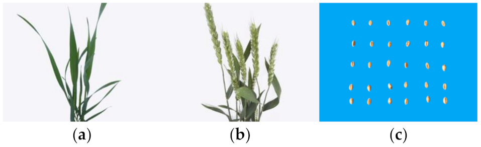
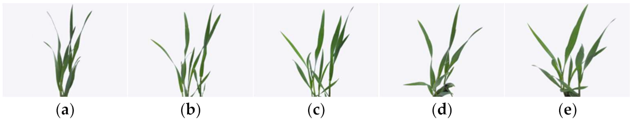
2.1. Wheat Images Data Analysis

The wheat image data of this paper were collected at the Tianshui Comprehensive Experimental Station of the National Wheat Industry Technology System in Qingshui County, Tianshui City, Gansu Province, China (latitude: 35°44′ N; longitude: 106°08′ E; average altitude: 1413 m; annual average rainfall: 570 mm; annual average sunshine: 2012 h). The collected wheat varieties are all mainstream varieties promoted in Gansu [13]. For capturing images in outdoor natural light, we used the automatic mode of the Nikon COOLPIX B700 digital camera, for which the highest ISO limit was 1600, the lowest shutter speed for shooting was 1/30 s, and the pictures were saved in JPG format. The image data collection time for the wheat tillering period was from 5–14 April 2021, there were 3 sunny days, 3 cloudy days, 2 days of light rain, and 2 cloudy days. The image data collection time for the flowering period of the wheat was from 15–20 May 2021; there was 1 sunny day, 3 cloudy days, and light rain for 1 day. The wheat seed image data collection time was from 15–20 July 2021; there were 3 sunny days, 1 cloudy day, and light rain for 1 day. The moisture content of all seeds at the time of shooting was between 7.5–10%. Parts of the tillering stage, flowering stage, and seed images are shown in Figure 1. In the shooting process, various weather conditions and natural lighting conditions were included, which increased the diversity of the captured images.
The 30 selected wheat varieties are all mainstream winter wheat varieties in Gansu Province, such as Jimai19, Lantian15, Zhoumai19, and so on. Approximately 30 plants were selected for each variety, and images were taken from multiple angles and aspects, such as top, side, distance, height, whole, and part. A total of 29,681 images were collected at the tillering stage, about 1000 for each variety; 14,482 pictures at the flowering stage, about 500 for each variety; and 4540 pictures of seeds, about 150 for each variety. The name information of each wheat variety is shown in Table 1.
The size of the pictures was mainly 1600 × 1200 pixels, and the naming method was “wheat variety abbreviation” + “-” + “plant number” + “-” + “camera view number”. For example, “LT54-34-1” represents the 34th plant of the wheat variety lantian54, a first-view photo. Taking the tillering stage as an example, part of the angle diagram is shown in Figure 2.

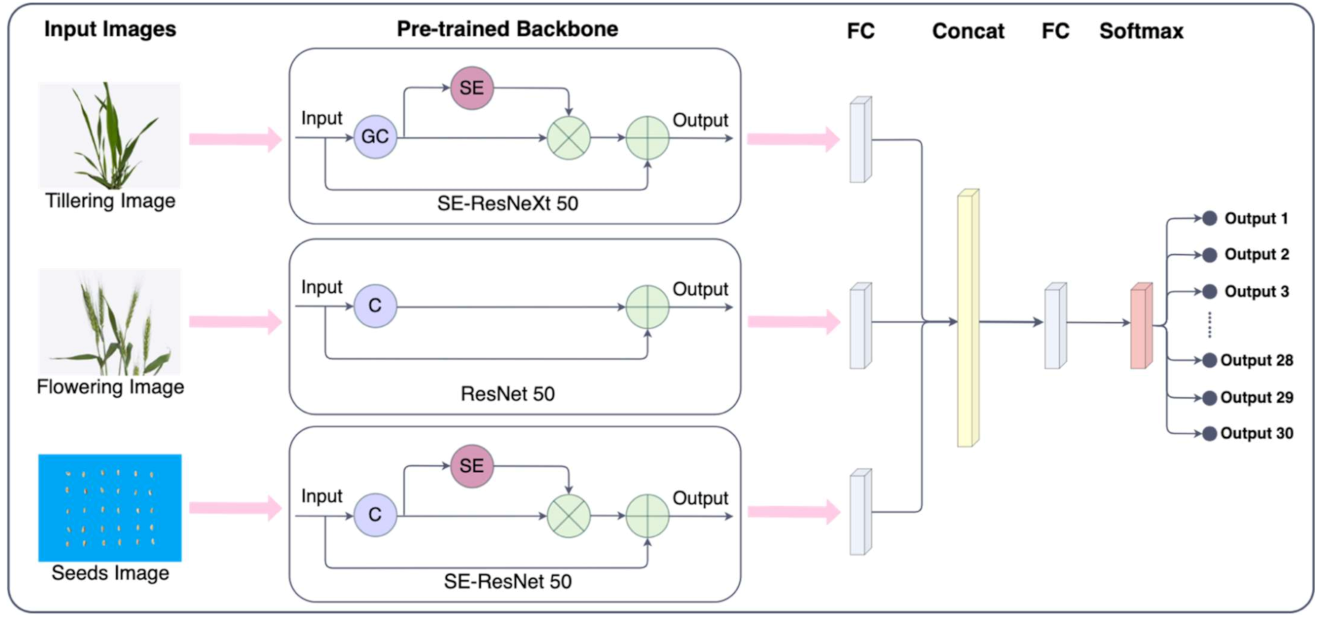
2.2. Wheat Images Deep Learning Model

Convolutional neural networks are an important part of image recognition in deep learning [14]. The convolutional layer is the core of a convolutional neural network that extracts image features [15]. A convolutional layer with superior performance can greatly improve the effect of a model. In theory, more features can be extracted by increasing the number of convolutional layers in a model. However, in practice, as the network depth increases, issues such as the vanishing gradient, exploding gradient, and degradation problems will occur [16]. A residual neural network, or ResNet, can effectively reduce the negative impact of these problems. ResNet is a stable and effective DCNN model. The residual structure it introduces can deepen the number of network layers while effectively reducing the impact of problems such as the vanishing gradient and enhance the relationship between the feature maps generated by different convolutional layers, thereby improving the recognition rate of a model. Figure 3 features the residual structure diagram of ResNet-50, which is mainly composed of two 1 × 1 convolutional layers used to adjust the number of feature map channels and a 3 × 3 convolutional layer used to extract features, as well as a shortcut structure and one feature map additive structure. These parts extract the characteristics of the input data, and at the same time make the input data propagate forward faster through a shortcut structure.
ResNet was proposed by He et al. [17]. Although the network performance is improved by increasing the number of network layers, the connection between different channels of the same feature map is ignored. The SE-Net model [18] is the champion of the image classification task in the ImageNet [19] Large-Scale Visual Recognition Challenge (ILSVRC). This network model introduces the attention mechanism into convolutional neural networks. A feature map usually consist of multiple feature channels. The model calculates the weight of each channel by learning the relationship between each feature channel, and then suppresses the noise in the feature map, so that the model can extract more useful information [20]. Figure 4 shows the residual structure diagram of SE-ResNet-50, which is mainly composed of squeeze, excitation, and scale. These three parts complete the self-adaptive calibration of the characteristic channel. The bypass includes a global average pooling layer, two fully connected layers, and ReLU and sigmoid activation functions. When the feature map passes this bypass, the weight of each channel will be learned and the residual output feature map and weight will be weighted to highlight the useful information in the feature map, suppress noise, and enhance the expressive ability of the model.
F s q U c = 1 H W i = 1 H j = 1 W U c i , j
In the squeeze operation, the global average pooling layer is used to compress each characteristic channel into a real number in order to describe the channel. This real number contains the global receptive field of the channel. The calculation formula is shown in Formula (1), where F s q U c represents the squeeze operation on the one channel of feature map U c , H is the height of the feature matrix, and W is the width of the feature matrix. Then, through a fully connected layer, the feature dimension is reduced, and after the ReLU activation function [21] is processed, the feature dimension is restored through a fully connected layer. In order to make the model have a stronger non-linear expression ability, and thereby better fit the complex correlation between the channels while reducing the model parameters and the amount of calculation, the excitation operation is used. The normalized weight of the output of the previous layer is obtained through the sigmoid activation function [22], and then the normalized weight is weighted to each channel through the scale operation. The squeeze and excitation (SE) operations provide a new method for reducing the complexity of the network, and introduce the attention mechanism into CNNs, making these better than other networks in obtaining the global receptive field.
ResNeXt [23] draws on the idea of the inception structure in GoogLeNet [24], extracts the information of different scales of the image through multiple convolution kernels, and fuses this information to obtain a better feature map representation, enhance the feature expression ability of the model, and improve the performance of the model. ResNeXt replaces traditional convolution with group convolution. Each group uses different convolution kernels for feature extraction. To reduce the complexity of the model structure, each group of convolutional layers adopts a similar structure. The number of groups can be controlled by setting hyperparameters. As shown in Figure 5, the SE-ResNeXt-50 residual structure uses 32 groups of convolution structures. ResNeXt broadens the network through group convolution, learns data features in a more structured way, and has stronger characterization capabilities. Figure 5 features the residual structure diagram of SE-ResNeXt-50. To obtain the residual structure of SE-ResNetXt-50, the convolutional layer in the bottleneck in the residual structure of SE-ResNet-50 is replaced with a group convolutional structure with a group number of 32.

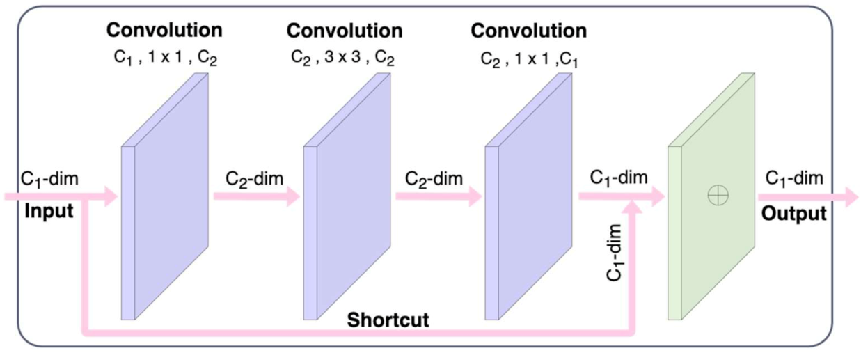
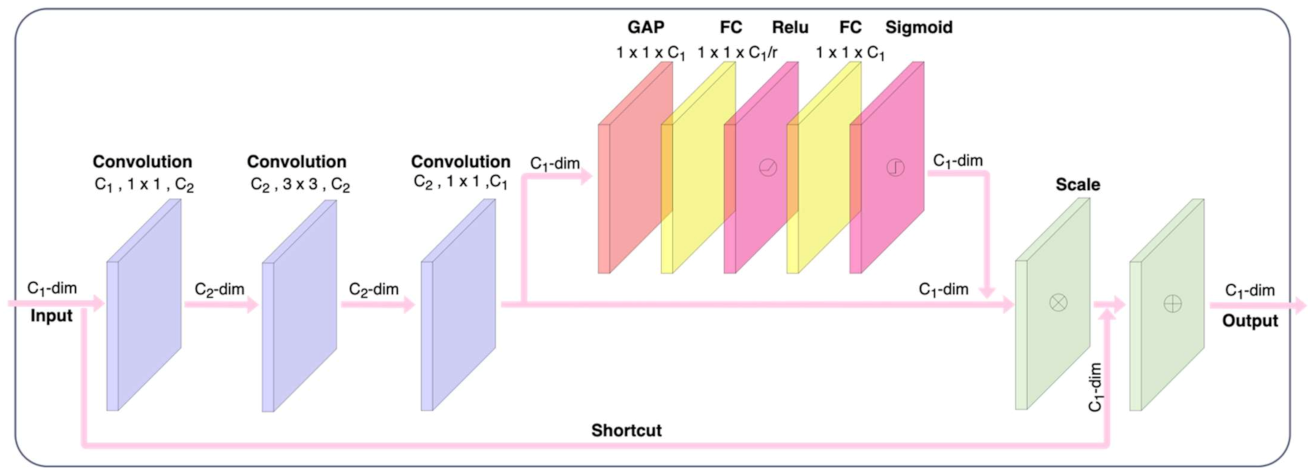
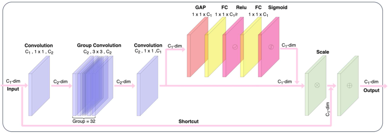
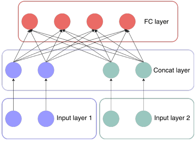
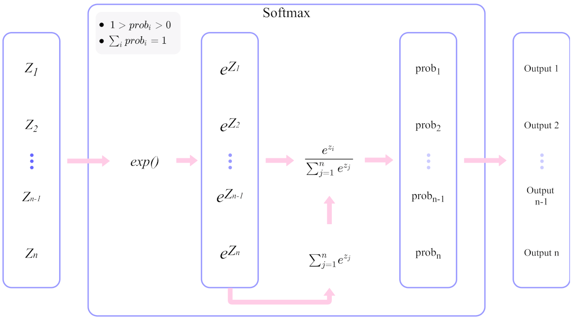
2.3. Network Structure Design

Based on transfer learning, this paper combines the ResNet-50, SE-ResNet-50, and SE-ResNeXt-50 models, and proposes a CMPNet model to improve the accuracy of the model’s identification of wheat varieties. The number of the parameters of these four models are as follows: CMPNet has 75.4 M parameters, SE-ResNeXt-50 has 25.6 M parameters, ResNet-50 has 23.6 M parameters, and SE-ResNet-50 has 26.2 M parameters. This model has a symmetrical structure along the horizontal direction. The CMPNet model draws on the ideas of random forest algorithms, a strong learner, turning the model into a coupled network composed of three independent networks. Figure 6 shows the structure of the CMPNet model. The model has three input terminals: pictures of the wheat tillering stage, pictures of the wheat flowering stage, and pictures of the wheat seeds. Since the wheat seeds were small, 30 wheat seeds were placed on a blue-purple background in a 5 × 6 format. Since the color of most wheat seeds is complementary to blue-violet [25], the color contrast was at its greatest, and the separation was strong, which is conducive to the model’s feature extraction of seeds, so blue-violet was selected as the background.
Through continuous experiments, which comprehensively assessed the model training time, model recognition accuracy, and model parameters, different network models were used to extract image features of different wheat growth periods. The tillering stages of different varieties of wheat were relatively similar, especially the seed pictures; the characteristics were difficult to extract. Therefore, the SE-ResNeXt-50 and SE-ResNet-50 models with the SE module and the group convolution module and only the SE module were used, respectively. Although these two models have slightly more trainable parameters compared to the ResNet model, and occupy more system resources, the SE module can adaptively correct the attention of the features, the calculation amount and scale are relatively small, the group convolution for different groups in the module can learn more and different feature representations, and, compared with ordinary convolution, the number of trainable parameters is slightly reduced; through these attributes, the model gained stronger characterization capabilities. Based on the theoretical analysis and experimental results, the SE-ResNeXt-50 and SE-ResNet-50 models were finally selected to extract the features of the wheat tillering stage and seed image data. The characteristics of different varieties of wheat are the most obvious in the flowering period, so the ResNet-50 model, with a low parameter quantity and low system resource occupation, was selected as the backbone. Before the model started training, the parameters obtained after each sub-model training process on the ImageNet dataset were reloaded into each sub-model, and the 1000-dimensional, fully connected layer and its softmax function were replaced [26] so that each sub-model finally passed with a 30-dimensional, fully connected layer. After each fully connected layer, the concat layer was used [27] to connect the three 30-dimensional fully connected layers end-to-end to obtain a 90-dimensional tensor, and then a layer of 30-dimensional, fully connected layers was connected. Finally, the softmax function was used to perform classification and to obtain the final classification result.
The concat layer structure featured in Figure 7 shows the end-to-end connection process of two two-dimensional tensors. In order to connect the two-dimensional tensors of the two input ends with the fully connected layer of the latter layer, the two-dimensional tensors of the two inputs were connected through the concat layer in the direction of the spliced four-dimensional layer. The tensor was connected to the four-dimensional, fully connected layer of the latter layer, and the activation function was not used in the process of splicing and connecting with the fully connected layer. In this way, the outputs of the three sub-models were spliced together to prepare for the final classification result.
Figure 8 shows the softmax function of the last fully connected layer of the model, through which the model classification results can be output in a probabilistic manner. The softmax function is used for multi-classification tasks. It can map the output of multiple neurons in the model to the 0 to 1 interval, and assign a probability value to the result of each output classification, indicating the possibility of it belonging to each category, thereby completing the multi-classification task. Formula (2) is the expression of the softmax function, where zi is the output value of the i-th node, and n is the number of output nodes. After calculation by the softmax function, the output of the model can be transformed into a probability distribution, and the probabilities of all nodes will add up to 1.
S o f t m a x z i = e z i j = 1 n e z j

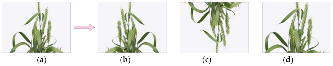
2.4. Data Preprocessing and Enhancement

To ensure the stability of the model during operation, reduce the model’s dependence on some irrelevant features, and improve the generalization ability of the model, data processing was required. In the original image, the storage space of a single image at either the tillering or flowering stages of wheat was about 600 KB, and the storage space of a single seed image was about 4 MB. Enhancing the image while ensuring the data feature information is retained can also increase the amount of training data. Figure 9 illustrates several data enhancement methods. The image was flipped horizontally and vertically through horizontal and vertical flip operations. Cropping was conducted to cut an image arbitrarily according to the ratio of 0.8–1.0 of the original image, and the size of the original image was upsampled. Among them, the image horizontal flip, vertical flip, 0.8–1.0 crop ratio selection, and image crop position all adopted the random mode triggered by probability. Finally, the image was scaled to the specified size for network loading.

3. Results and Discussion

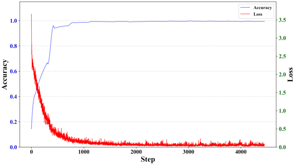
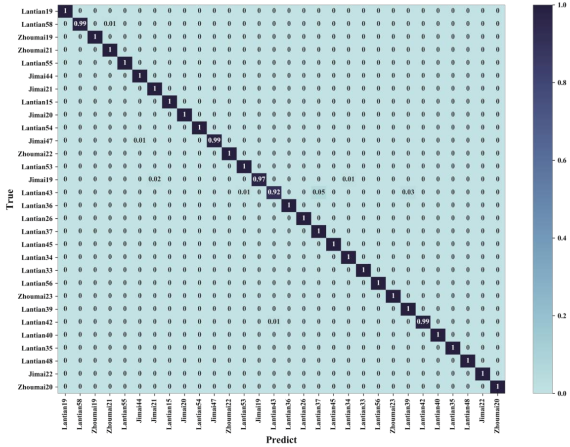
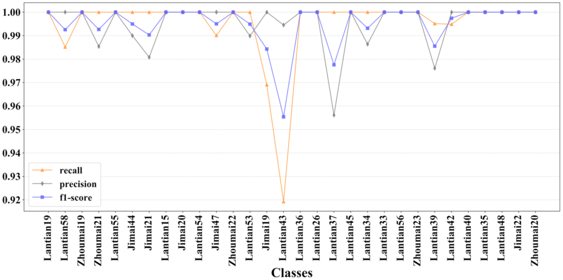
3.1. Result Analysis

According to the ratio of 8:2, the training dataset and the test dataset were randomly selected, and the image data of the wheat was enhanced by the data enhancement method shown in Figure 9. PiecewiseDecay [28] was used to set the learning rate of the model in segments. The specific values are shown in Table 2. The epoch was set to 12, the batch size was 64, the L2 regularization coefficient [29] was 0.2, and the cross-entropy loss function and the adaptive moment estimation optimization algorithm were used. This study used the Python3 language, the Ubuntu Linux system, a 4-core processor, 32 GB RAM, 100 GB of disk capacity, and a Nvidia Tesla V100 graphics card to accelerate the model training. The display storage capacity was 32 GB. The training configuration is shown in Table 3.
Figure 10 shows the loss and accuracy of the model training process as the number of training iterations increased. As the number of training iterations increased, the training loss rate showed a downward trend. Although the loss rate in part of the training phase did not decrease but rather increased, the overall loss rate was in a declining state and quickly converged, and finally oscillated at around 0.08 without decreasing. Furthermore, as the number of training iterations increased, the training accuracy rate also increased. When the number of iterations reached about 1100, the model was very close to the local optimal solution in the solution space, and the training accuracy also tended to converge. Since the PiecewiseDecay learning rate was used, each piecewise learning rate could allow the optimization to proceed to a state where the weight vector distribution was relatively stable, in order to obtain a better local minimum. It can be seen from Figure 10 that the training accuracy curve dropped several times during the rising process, but the model finally deepened the learning of the data, overcame the trap of local optimization, further improved the wheat identification accuracy, and finally stabilized. It can be seen that the model continuously adjusted the parameters, and the learning effect was continuously improved.
Table 4 shows the accuracy of the model on the training dataset and test dataset. After a long period of training, the top-1 accuracy of the training dataset reached 100%. At this time, the top-1 accuracy of the test dataset reached 99.51%, and the top-2 accuracy of the training dataset and test dataset reached 100% and 99.83%, respectively. The performance of the CMPNet model proposed in this paper was good, and the recognition accuracy on the test dataset was excellent.
To further verify the model, the generalization ability and robustness of the model was tested. The test dataset was used to test the trained model, and a confusion matrix [30] was used to visualize the model test results. Figure 11 shows the classification confusion matrix for the 30 wheat varieties. In the confusion matrix, the horizontal axis represents the prediction results of the model, the vertical axis represents the true category of wheat varieties, the elements on the main diagonal represent the percentage of correct model recognition, and the remaining positions represent the percentage of model recognition errors. It can be seen from the figure that the recognition rates of Lantian58, Jimai47, Jimai19, Lantian43, and Lantian42 were all lower than the overall level. Among them, the recognition accuracy of Lantian43 was the worst, only 91.9192%. By analyzing the confusion matrix, we knew that Lantian43 was most likely to be misclassified as Lantian37. In the testing process of the remaining 25 varieties, the model successfully predicted almost all test samples, with an accuracy rate of about 100%, for Lantian45, Jimai20, ZhouMai21, and so on.
As shown in Table 5, the model classification evaluation index was used to further analyze the model performance. Precision (P) means the prediction result was the proportion of the true label in the positive sample that was positive; recall (R) means the true label was the proportion of positive examples in the sample whose prediction results were positive; and F1-score means the result was the harmonic average of the precision and recall, reflecting the robustness of the model.
As shown in Figure 12, combining the above confusion matrix and the model classification evaluation indicators, the precision, recall, and F1-score of the model on the test dataset can be calculated, respectively. When only considering the precision rate, the model had the worst recognition ability for Lantian43, followed by Jimai19; Lantian45, Jimai20, and Zhoumai21 had the best recognition results. If the precision rate and the recall rate are considered comprehensively, and the precision rate and the recall rate are equally important, ( β = 1 ); that is, in the case of the F1-score, the model’s ability to recognize Lantian43 was also the worst. The second worst was Lantian37, indicating that the model needs to improve the extraction of Lantian43 features.
At the same time, the optimal relationship between the model performance and calculation time during the model design was weighed. After the system loaded the model, by calculating the reasoning speed of the model on the test dataset, it was concluded that the model predicted that a single set of pictures only needed about 0.0212 s, which can meet the actual project requirements. Comparing the sub-models, although the time was slightly higher, the accuracy was better.

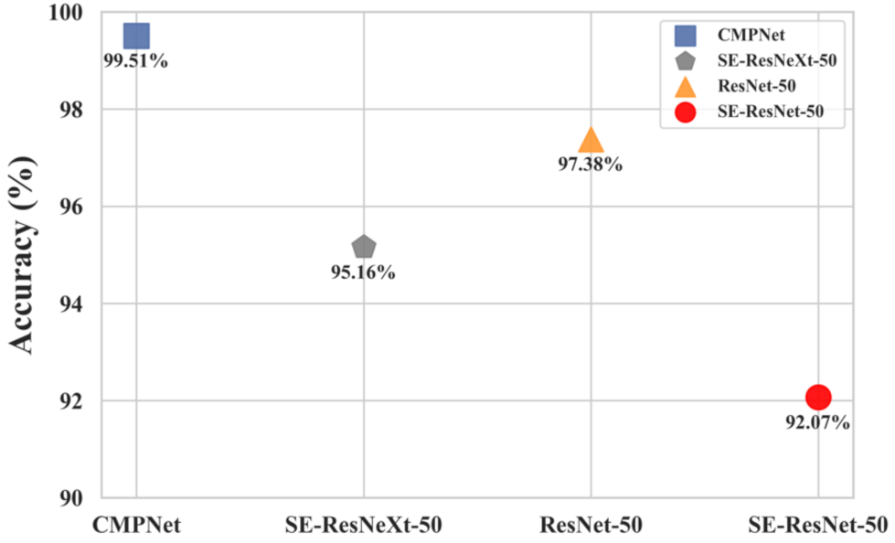
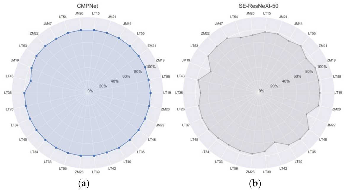
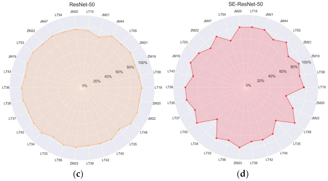
3.2. Comparison with Single Models

The corresponding wheat image test dataset was input into the sub-model, and the classification results were statistically analyzed to obtain the average accuracy rate of the wheat classification and recognition of each sub-model, as shown in Figure 13. The average accuracy of each model was above 92%, indicating that the deep learning model performed excellently in the classification and recognition of wheat varieties. At the same time, CMPNet achieved an average accuracy of 99.51% on the test dataset, which was 4.35%, 2.13%, and 7.44% higher than that of the SE-ResNeXt-50, ResNet-50, and SE-ResNet-50 models, respectively. The test dataset of SE-ResNeXt-50 was a picture of wheat at the tillering period, the test dataset of ResNet-50 was a picture of a wheat at the flowering period, and the test dataset of SE-ResNet-50 was a picture of wheat seeds.
Each model was tested on the wheat image test dataset, and the accuracy rate of the 30 wheat varieties was obtained. Figure 14 shows the test results of each model on the 30 wheat varieties; there are 30 wheat varieties on the circle, and the length of the radius is the precision. The accuracy of the model for each wheat variety is expressed in the form of polar coordinates. Each point on the polar coordinates is connected to the drawn convex hull in turn. The closer it was to a circle with a radius of 100%, the stronger the overall recognition ability of the model. The accuracy of the model on each wheat variety was used to draw the convex hull. When the drawn convex hull was closer to a circle with a radius of 100%, the model had a better overall recognition accuracy for each wheat variety. It can be seen from the figure that CMPNet had a stronger generalization ability than the other models, and the recognition accuracy was also greatly improved. In addition to the relatively poor recognition ability of Lantian43, the recognition ability for the other varieties was also greatly improved, such as for Lantian35, Zhoumai21, etc.; some varieties, such as Jimai47, performed well in the recognition process of each model. To summarize, the results showed that the CMPNet model mainly corrected the errors of each sub-model in the classification and recognition processes.

4. Conclusions

This paper proposes a variety classification recognition model based on deep learning combined with images of multiple growth periods of wheat. CMPNet was used, which realized high-precision classification and recognition of the wheat varieties and improved the accuracy of wheat classification. Taking the image data as the core, based on the transfer learning method of the SE-ResNeXt-50, ResNet-50, and SE-ResNet-50 models, image recognition models for the wheat tillering stage, wheat flowering stage and wheat seeds were constructed, respectively, then the models were combined to improve the accuracy and generalization ability of the model. The method uses migration learning, and some local optimal solutions stored in the pre-training parameters do not need to be retrained, reducing the model training time and cost. The training dataset contained images of different growth periods of wheat, which solved the problem of the single characteristics of wheat and ensured the reliability of the model. Through comparative experiments with each sub-model, it was found that the coupled model mainly corrected the errors of each sub-model in the classification and recognition processes and ensured the generalization ability of the model. The SE-ResNeXt-50, ResNet-50, and SE-ResNet-50 models were used to extract the image features of each growth stage of wheat, and the softmax layer of the model was retrained to obtain a wheat image classification model. The test dataset was used to test the generalization ability of the model, and the final test accuracy rates were 95.16%, 97.38%, and 92.07%, respectively. The sub-models were coupled with each other to make full use of the characteristics of the different growth periods of wheat. The final coupling recognition rate was 99.51%, which was higher than the recognition rate of each sub-model, indicating that the coupling model had a stronger accuracy and robustness.
Our future work will mainly be divided based on four considerations: (i) the interaction of biological genes and environment means the same crop variety may present different forms in different production environments. Consequently, the precondition of the model’s localized application is the model training must use the data in the corresponding production environment. Our team’s cross-regional morphological recognition experiment of the same species has not been carried out yet. At present, it is possible to reduce the adverse effects of this problem on the model performance by continuously adding images of the same variety of wheat across regions to the training data set. (ii) In order to give full play to the model’s advantages in classification speed and accuracy, we will deploy the model to portable electronic terminals like mobile phones to realize rapid and timely classification of the photos we take in the future, with which the model’s superiority will be fully displayed. (iii) In view of the generally poor recognition rate of wheat seeds, our follow-up research will collect more data and improve the model algorithm according to the various characteristics of wheat. (iv) By studying other deep neural network models, such as Swin Transformer [31], HRNet [32], BotNet [33], etc., the recognition accuracy for a single growth period of wheat should be improved, and we will consider transplanting the model to the variety recognition of other crops. Lastly, we provide the source code of CMPNet, which can be accessed at https://github.com/GaoJiameng/CMPNet (accessed on 1 September 2021).

Author Contributions

Conceptualization, C.L.; data curation, J.G., C.L., X.B. and J.L.; formal analysis, C.L.; funding acquisition, C.L., J.H. and J.Z.; investigation, J.G., C.L. and J.H.; methodology, J.G. and C.L.; project administration, C.L.; resources, Q.L. and H.W.; software, J.G.; supervision, C.L., J.H., Q.L., H.W. and J.Z.; validation, J.G., C.L., X.B. and J.L.; visualization, J.G.; writing—original draft, J.G.; writing—review and editing, J.G. and C.L. All authors have read and agreed to the published version of the manuscript.

Funding

This work was supported by the Innovation Fund Project of Colleges and Universities in Gansu of China (Grant No.2021A-056); by the Natural Science Foundation of Gansu Province, China (Grant No.20JR5RA023); by the Industrial Support and Guidance Project of Universities in Gansu Province, China (Grant No.2021CYZC-57); and by the National Natural Science Foundation of China (Grant No.31971792).

Acknowledgments

We are grateful for the anonymous reviewers’ hard work and comments, which allowed us to improve the quality of this paper.

Conflicts of Interest

The authors declare that they have no known competing financial interests or personal relationships that may influence the work reported in this paper.

References

  1. Charmet, G. Wheat domestication: Lessons for the future. Comptes Rendus Biol. 2011, 334, 212–220. [Google Scholar] [CrossRef] [PubMed]
  2. OECD. Crop Production; OECD: Paris, France, 2018. [Google Scholar]
  3. Peng, J.; Sun, D.; Nevo, E. Wild emmer wheat, Triticum dicoccoides, occupies a pivotal position in wheat domestication process. Aust. J. Crop. Sci. 2011, 5, 1127–1143. [Google Scholar]
  4. Salsman, E.; Liu, Y.; Hosseinirad, S.A.; Kumar, A.; Manthey, F.; Elias, E.; Li, X. Assessment of genetic diversity and agronomic traits of durum wheat germplasm under drought environment of the northern Great Plains. Crop. Sci. 2021, 61, 1194–1206. [Google Scholar] [CrossRef]
  5. Drywa, A.; Poćwierz-Kotus, A.; Dobosz, S.; Kent, M.P.; Lien, S.; Wenne, R. Identification of multiple diagnostic SNP loci for differentiation of three salmonid species using SNP-arrays. Mar. Genom. 2014, 15, 5–6. [Google Scholar] [CrossRef] [PubMed]
  6. Priya, C.A.; Balasaravanan, T.; Thanamani, A.S. An efficient leaf recognition algorithm for plant classification using support vector machine. In Proceedings of the 21st International Conference on Pattern Recognition, Tsukuba, Japan, 11–15 November 2012; pp. 428–432. [Google Scholar] [CrossRef]
  7. Wang, Z.; Sun, X.; Zhang, Y.; Ying, Z.; Ma, Y. Leaf recognition based on PCNN. Neural Comput. Appl. 2016, 27, 899–908. [Google Scholar] [CrossRef]
  8. Liu, C.; Han, J.; Chen, B.; Mao, J.; Xue, Z.; Li, S. A novel identification method for apple (Malus domestica Borkh.) cultivars based on a deep convolutional neural network with leaf image input. Symmetry 2020, 12, 217. [Google Scholar] [CrossRef] [Green Version]
  9. Sabadin, F.; Galli, G.; Borsato, R.; Gevartosky, R.; Campos, G.R.; Fritsche-Neto, R. Improving the identification of haploid maize seeds using convolutional neural networks. Crop. Sci. 2021. [Google Scholar] [CrossRef]
  10. Ahmed, E.; Moustafa, M. House price estimation from visual and textual features. In Proceedings of the NCTA 8th International Conference on Neural Computation Theory and Applications, Porto, Portugal, 9–11 November 2016. [Google Scholar]
  11. Quan, S.; Bernhard, P. Bagging ensemble selection for regression. In Proceedings of the Australasian Joint Conference on Advances in Artificial Intelligence, Sydney, NSW, Australia, 4–7 December 2012. [Google Scholar]
  12. Breiman, L. Random forest. Mach. Learn. 2001, 45, 5–32. [Google Scholar] [CrossRef] [Green Version]
  13. Zhou, G.; Zhang, W.; Lu, Q.; Bai, Y.; Wang, H.; Zhang, Y.; Zhang, L. Analysis and Evaluation on Quality of Winter Wheat Varieties from Gansu Province. J. Triticeae Crop. 2019, 39, 46–51. [Google Scholar]
  14. Yoo, H.J. Deep convolution neural networks in computer vision. IEIE Trans. Smart Process. Comput. 2015, 4, 35–43. [Google Scholar] [CrossRef]
  15. Nikhil, K. Deep Learning with Python; Apress: Barkeley, CA, USA, 2017. [Google Scholar]
  16. Youm, G.Y.; Bae, S.H.; Kim, M. Image super-resolution based on convolution neural networks using multi-channel input. In Proceedings of the 2016 IEEE 12th Image, Video, and Multidimensional Signal Processing Workshop (IVMSP), Bordeaux, France, 11–12 July 2016. [Google Scholar]
  17. He, K.; Zhang, X.; Ren, S.; Sun, J. Deep residual learning for image recognition. In Proceedings of the 2016 IEEE Conference on Computer Vision and Pattern Recognition (CVPR), Las Vegas, NV, USA, 27–30 June 2016; pp. 770–778. [Google Scholar]
  18. Hu, J.; Shen, L.; Albanie, S.; Sun, G.; Wu, E. Squeeze-and-Excitation Networks. IEEE Trans. Pattern Anal. Mach. Intell. 2020, 42, 2011–2023. [Google Scholar] [CrossRef] [Green Version]
  19. Deng, J.; Dong, W.; Socher, R.; Li, L.-J.; Li, K.; Li, F.-F. ImageNet: A Large-Scale Hierarchical Image Database. In Proceedings of the 2009 IEEE Conference on Computer Vision and Pattern Recognition, Miami, FL, USA, 20–25 June 2009; pp. 248–255. [Google Scholar]
  20. Ma, H.; Han, G.; Peng, L.; Zhu, L.; Shu, J. Rock thin sections identification based on improved squeeze-and-Excitation Networks model. Comput. Geosci. 2021, 152, 104780. [Google Scholar] [CrossRef]
  21. Eckle, K.; Schmidt-Hieber, J. A comparison of deep networks with ReLU activation function and linear spline-type methods. Neural Netw. 2018, 110, 232–242. [Google Scholar] [CrossRef] [PubMed]
  22. Jie, H.; Zeng, X. An Efficient Activation Function for BP Neural Network. In Proceedings of the International Workshop on Intelligent Systems and Applications ISA, Wuhan, China, 23–24 May 2009. [Google Scholar]
  23. Xie, S.; Girshick, R.; Dollár, P.; Tu, Z.; He, K. Aggregated Residual Transformations for Deep Neural Networks. In Proceedings of the 2017 IEEE Conference on Computer Vision and Pattern Recognition (CVPR), Honolulu, HI, USA, 21–26 July 2016. [Google Scholar]
  24. Szegedy, C.; Liu, W.; Jia, Y.; Sermanet, P.; Reed, S.; Anguelov, D.; Erhan, D.; Vanhoucke, V.; Rabinovich, A. Going deeper with convolutions. In Proceedings of the 2015 IEEE Conference on Computer Vision and Pattern Recognition (CVPR), Boston, MA, USA, 7–12 June 2015; pp. 1–9. [Google Scholar] [CrossRef] [Green Version]
  25. Pridmore, R.W. Complementary colors theory of color vision: Physiology, color mixture, color constancy and color perception. Color Res. Appl. 2011, 36, 394–412. [Google Scholar] [CrossRef]
  26. Bouchard, G. Clustering and Classification Employing Softmax Function Including Efficient Bounds. U.S. Patent 8,065,246, 22 November 2011. [Google Scholar]
  27. Gao, Z.; Xue, H.; Wan, S. Multiple discrimination and pairwise CNN for view-based 3D object retrieval. Neural Netw. 2020, 125, 290–302. [Google Scholar] [CrossRef] [PubMed] [Green Version]
  28. Wu, P.; Yeung, C.H.; Liu, W.; Jin, C.; Zhang, Y.-C. Time-aware collaborative filtering with the piecewise decay function. arXiv 2010, arXiv:1010.3988v1. [Google Scholar]
  29. Wen, J.; Lai, Z.; Wong, W.K.; Cui, J.; Wan, M. Optimal feature selection for robust classification via l2,1-norms regularization. IEEE Comput. Soc. 2014, 517–521. [Google Scholar] [CrossRef]
  30. Li, M.; Fu, J.; Zhang, Y.; Liu, C. Intelligent recognition and analysis method of rock lithology classification based on coupled rock images and hammering audios. Chin. J. Rock Mech. Eng. 2020, 39, 137–145. [Google Scholar]
  31. Liu, Z.; Lin, Y.; Cao, Y.; Hu, H.; Wei, Y.; Zhang, Z.; Lin, S.; Guo, B. Swin transformer: Hierarchical vision transformer using shifted windows. arXiv 2021, arXiv:2103.14030v2. [Google Scholar]
  32. Sun, K.; Zhao, Y.; Jiang, B.; Cheng, T.; Xiao, B.; Liu, D.; Mu, Y.; Wang, X.; Liu, W.; Wang, J. High-resolution representations for labeling pixels and regions. arXiv 2019, arXiv:1904.04514v1. [Google Scholar]
  33. Srinivas, A.; Lin, T.-Y.; Parmar, N.; Shlens, J.; Abbeel, P.; Vaswani, A. Bottleneck transformers for visual recognition. arXiv 2021, arXiv:2101.11605v2. [Google Scholar]
Figure 1. Wheat multi-growth period samples: (a) the tillering period of wheat, (b) the flowering period, and (c) the seed period.
Symmetry 13 02012 g001
Figure 2. Partial angle pictures of the tillering period. The names of the pictures from (ae) are LT54-34-1.jpg, LT54-34-5.jpg, LT54-34-10.jpg, LT54-34-15.jpg, and LT54-34-20.jpg.
Symmetry 13 02012 g002
Figure 3. Residual structure diagram of ResNet-50. Two 1 × 1 convolutional layers are used to adjust the number of channels of the feature map; the features in the feature map are extracted from the 3 × 3 convolutional layer.
Symmetry 13 02012 g003
Figure 4. Residual structure diagram of SE-ResNet-50. On the basis of the residual structure, the SE module is added to make the model obtain the attention mechanism, which focuses on extracting the features of the channel with a higher weight.
Symmetry 13 02012 g004
Figure 5. Residual structure diagram of SE-ResNeXt-50. It uses 32 groups of group convolution to replace the 3 × 3 convolutional layer in SE-ResNet in order to obtain the residual structure diagram of SE-ResNeXt.
Symmetry 13 02012 g005
Figure 6. CMPNet network structure. Images of different growth periods of the same varieties were input from the input layer of the model at the same time, and after the backbone performed parallel feature extraction of data based on transfer learning, three tensors, each with a length of 30 dimensions, were obtained, which were spliced by the Concat function and combined with one 30-dimensional layer. After the fully connected layers of the 30 dimensions were connected, the softmax function was used to obtain the classification result.
Symmetry 13 02012 g006
Figure 7. Concat layer structure. By concatenating two tensors from the input layer at the end, they are combined into one tensor.
Symmetry 13 02012 g007
Figure 8. Softmax layer structure. The exponent with e as the base of the input tensor was calculated, and the result was the numerator. The numerator was added and the denominator was obtained, and the probability output was then attained after the division operation.
Symmetry 13 02012 g008
Figure 9. Data enhancement strategy: (a) the original image, (b) the horizontal flip image, (c) the vertical flip image, and (d) the cropped image.
Symmetry 13 02012 g009
Figure 10. Curves of training loss and training accuracy. The vertical axis on the left (blue) is the training accuracy, the vertical axis on the right (red) is the training loss, and the horizontal axis is the number of training iteration steps.
Symmetry 13 02012 g010
Figure 11. Confusion matrix for classification. The values range from 0 to 1. The closer to 1, the darker the color of the grid. Due to the image size limitation, only two decimal places are displayed.
Symmetry 13 02012 g011
Figure 12. Evaluation index of CMPNet model classification. The horizontal axis is the 30 wheat varieties, the vertical axis is the value of the model evaluation index, and the value range is 0–1.
Symmetry 13 02012 g012
Figure 13. Comparison of the average recognition accuracies of the model. The horizontal axis features the models that participated in the test. The vertical axis features the top-1 accuracy of the model on the respective test dataset, and the accuracy value range is 0–100%.
Symmetry 13 02012 g013
Figure 14. Comparison of the identification accuracies of the different varieties in each model. (a) CMPNet: the input data is wheat tillering period, flowering period, and seed image data; (b) SE-ResNeXt-50: the input data is wheat tillering period image data; (c) ResNet-50: the input data is wheat flowering period image data; and (d) SE-ResNet-50: the input data is seed image data.
Symmetry 13 02012 g014aSymmetry 13 02012 g014b
Table 1. The 30 wheat varieties used in this paper, divided into three cultivars (lines): Lantian, Jimai, and Zhoumai.
Cultivar (Lines)Variety
LantianLantian15Lantian36Lantian45
Lantian19Lantian37Lantian48
Lantian26Lantian39Lantian53
Lantian33Lantian40Lantian54
Lantian34Lantian42Lantian55
Lantian35Lantian43Lantian56
Lantian58
JimaiJimai19Jimai21Jimai44
Jimai20Jimai22Jimai47
ZhoumaiZhoumai19Zhoumai21Zhoumai23
Zhoumai20Zhoumai22
Note. Among them, Lantian has 19 varieties, Jimai has 6 varieties, and Zhoumai has 5 varieties.
Table 2. PiecewiseDecay superparametrics. The learning rate was divided into four segments, in the order of 0.0005, 0.0001, 0.00002, and 0.00001.
Learning RateStep Interval
0.0005[1, 5]
0.0001(5, 10]
0.00002(10, 15]
0.00001(15, 4452]
Note. The learning rate decreased continuously from 0.0005 to 0.00001 as the number of model training steps increased. The initial learning rate was large, which can improve the convergence speed of the model, and the later learning rate was small, which can stabilize the training results of the model and reduce the possibility of the model missing the optimal solution.
Table 3. Training configuration information.
Configuration Information
OSUbuntu Linux
CPU4 Cores
RAM32 GB
Disk100 GB
GPUTesla V100
Video Memory32 GB
Note. Tesla V100 is a graphics card with a large number of high-performance floating-point computing units.
Table 4. CMPNet model accuracy.
Training Dataset Accuracy (%)Test Dataset Accuracy (%)
Top-1 Accuracy10099.51
Top-2 Accuracy10099.83
Note. Top-1 accuracy refers to the accuracy rate of the first category in line with the actual results, while top-2 accuracy refers to the accuracy rate of the top two categories containing the actual results.
Table 5. The formula of the evaluation index of model classification.
Model IndexFormula
Precision P = T P T P + F P
Recall R = T P T P + F N
F1-score F β = P R 1 + β 2 β 2 P + R , β = 1
Note. True positive (TP) means that the prediction was correct, the true value was a positive example, and the model predicted a positive example; true negative (TN) means that the true value was a negative example, and that the model predicted a negative example; false positive (FP) means the true value was a negative example, and the model predicted a positive example; false negative (FN) means the true value was a positive example, and the model predicted a negative example.
Publisher’s Note: MDPI stays neutral with regard to jurisdictional claims in published maps and institutional affiliations.

