Constitutive Equations for Magnetic Active Liquids

Abstract

This article is focused on the derivation of constitutive equations for magnetic liquids. The results can be used for both ferromagnetic and magnetorheological fluids after the introduced simplifications. The formulation of constitutive equations is based on two approaches. The intuitive approach is based on experimental experience of non-Newtonian fluids, which exhibit a generally non-linear dependence of mechanical stress on shear rate; this is consistent with experimental experience with magnetic liquids. In these general equations, it is necessary to determine the viscosity of a liquid as a function of magnetic induction; however, these equations only apply to the symmetric stress tensor and can only be used for an incompressible fluid. As a result of this limitation, in the next part of the work, this approach is extended by the asymmetry of the stress tensor, depending on the angular velocity tensor. All constitutive equations are formulated in Cartesian coordinates in 3D space. The second approach to determining constitutive equations is more general: it takes the basis of non-equilibrium thermodynamics and is based on the physical approach, using the definition of density of the entropy production. The production of entropy is expressed by irreversible thermodynamic flows, which are caused by the effect of generalized thermodynamic forces after disturbance of the thermodynamic equilibrium. The dependence between fluxes and forces determines the constitutive equations between stress tensors, depending on the strain rate tensor and the magnetization vector, which depends on the intensity of the magnetic field. Their interdependencies are described in this article on the basis of the Curie principle and on the Onsager conditions of symmetry.

1. Introduction

Electromagnetic hydrodynamics can be divided into three basic parts. The first deals with the interaction between the magnetic field and the conductive fluid. The solution mainly concerns homogeneous and isotropic liquids, whose volumes are acted on by the Lorentz force [1,2]. Homogeneous and isotropic liquids are used, for example, for the construction of special magnetic bearings and pumps, based on the principle of electrically conductive liquids [3,4,5]. The second part, so-called ferrohydrodynamics, investigates the interaction between a magnetic field and a flowing, magnetically polarized liquid [6,7,8,9,10,11,12]. The third part focuses on the flow of so-called electro-magnetorheological non-Newtonian fluids [6,7,13,14,15,16,17].

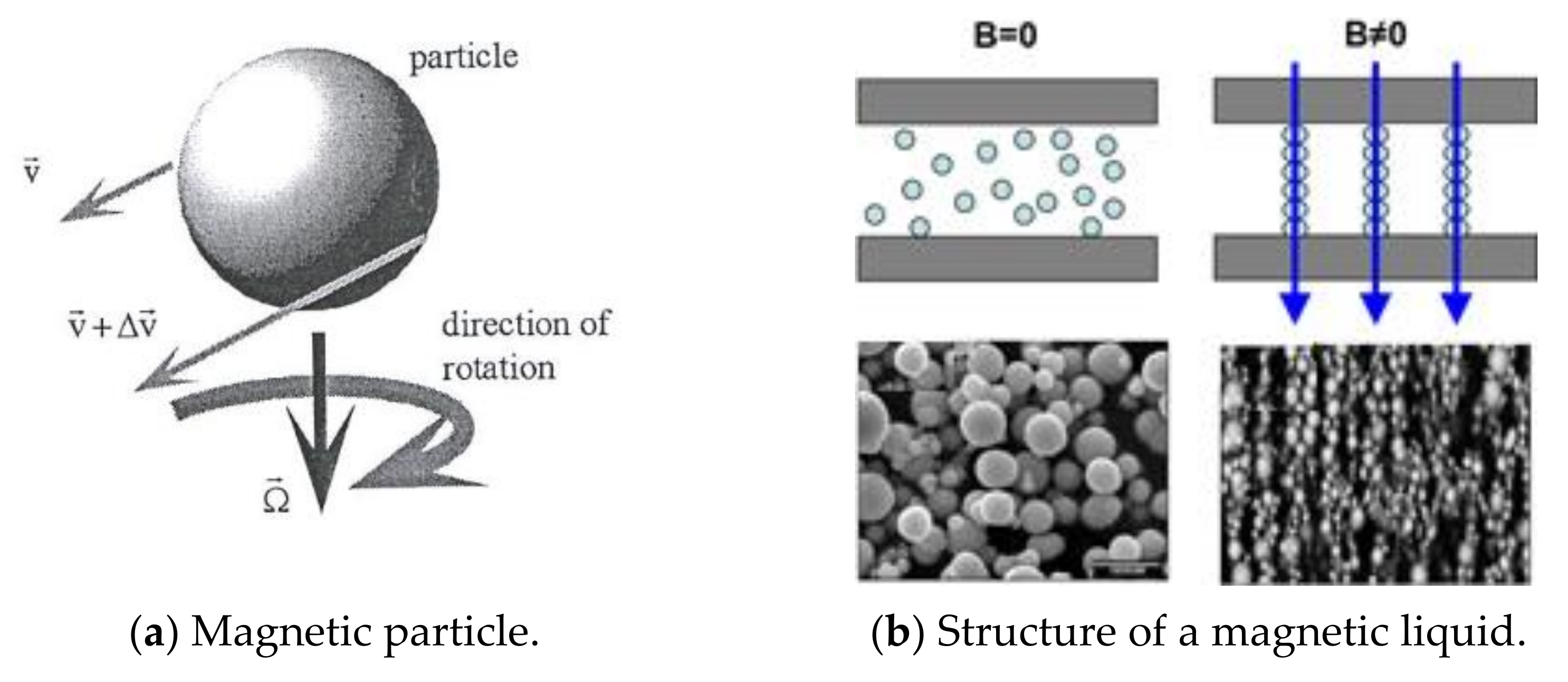
Liquids of the second and third classes are formed by a suspension of very fine ferromagnetic or ferrimagnetic particles (FM liquid) dispersed in a carrier liquid. If the particle size is of the order of nanoscale (≤6 nm) [3], the particles move in Brownian motion and are characterized by a magnetic moment. When exposed to a magnetic field, the nanoparticles polarize and twist in the direction of the magnetic field, which results in a change in the isotropy of the environment [6,7,18].

Particles of larger dimensions, of the order of micrometers, do not have a magnetic moment if they are not magnetically polarized. When a liquid is composed of these particles, it differs from ferrofluids mainly in its behavior, since the external magnetic field increases the viscosity of the particles; consequently, they are characterized by a strong magnetoviscous phenomenon, which usually gives the magnetic liquid a Bingham character [6,7,15,17]. This type of liquid is known as a magnetorheological liquid (MR liquid) [6,14,15,16]. These two types of liquids are mainly used for the construction of special hydrodynamic dampers and hydrodynamic seals [11,19,20,21,22].

The effect of the magnetic field, as already mentioned, leads to polarization of the particles. The movement of particles is very complicated, and during their interaction with the carrier liquid, due to particle rotation, asymmetry of the stress tensor occurs due to the angular velocity of the particles. The rotation induces additional surface forces in the carrier liquid, characterized by an additional tensor of mechanical stresses ${\mathsf{\Lambda }}_{ij }$ [7,23]. Changes in the viscosity, produced by the magnetic field and particle rotation, have a significant effect on the resulting mechanical irreversible stress tensor ${\mathsf{\sigma }}_{ij}$, which must be formulated in accordance with the rules of non-equilibrium thermodynamics [1,22,23,24,25].

For magnetic liquids containing particles, it is necessary to derive constitutive equations for an inhomogeneous liquid with more components (n), in which a number of chemical reactions (r) can take place in a non-isotropic environment [26,27,28].

As a result, constitutive equations may include the effects of diffusion, chemical reactions, magnetization, polarization, particle rotation, and temperature [7,22]. The solver considers the significance of individual influences for a given type of liquid and provides simplifications, with respect to the direction of the action of magnetic induction and the direction of the flow rate of the liquid. It should also be emphasized that the properties of FM liquids, especially MR liquids, depend on temperature. Technical applications can be realized at temperatures in the interval (−50 °C, 200 °C); however, it is necessary to consider the value of the Curie temperature, at which the magnetic properties of the liquid disappear.

It is also necessary to consider the use of magnetic liquids for structural elements operating under non-stationary loading. Depending on the time, the liquid heats up and produces significant changes in viscosity. These changes must be considered in mathematical and computational modeling.

The mentioned phenomena can occur especially in the construction of hydrodynamic dampers [11,19,20,21], but also seals [22] when operating under non-stationary loading, if a large volume of magnetic liquid is deformed without cooling.

Einstein summation convention is used in the article, where

$${\delta }_{ij}\hspace{1em}\hspace{1em}\hspace{1em}$$	Kronecker delta
$${\epsilon }_{ijk}$$	Levi-Civita tensor

2. Kinematics of the Motion of the Magnetic Liquid

When creating a mathematical model of MR liquid flow, it is necessary to know the resulting tensor of irreversible stresses ${\sigma }_{ij}$ and the volumetric magnetic force $F_{Mi}$—which is applied by the magnetic field to the liquid—which is the aim of this work. The general relation [1] applies to the electromagnetic force $F_{Ei}$:

$$F_{Ei}={\rho }_e{E}_i+{\epsilon }_{ijk}{j}_j{B}_k+\frac{\partial E_k}{\partial x_i}{P}_k+\frac{\partial H_k}{\partial x_i}{M}_k$$

(1)

${\rho }_e$ is a charge density, $E_i$ is an electric field intensity,$j_j$ is a current density,$B_k$ is a magnetic flux density, $P_k$ is a polarization, $H_k$ is a magnetic field intensity, and $M_k$ is a magnetization. In the case of non-conductive magnetic liquid, where $j_j=0$ and ${\rho }_e=0$, we obtain the following equation:

$$F_{Mi}=\frac{\partial H_k}{\partial x_i}{M}_k$$

(2)

If magnetization is colinear with intensity of magnetic field

$$M_k=\chi H_k$$

(3)

then the so-called Kelvin force can be written in the form:

$$F_{Mi}=\frac{\chi }{2}\frac{\partial }{\partial x_i}{H}^2, H^2=H_i{H}_i, M^2=M_i{M}_i$$

(4)

When solving the flow of a magnetic liquid (FM or MR), we start from the equations of equilibrium, in which the influence of external volume forces, represented by the Maxwell stress tensor, is considered. The magnetic liquid no longer behaves like a Newtonian liquid because the tensor of mechanical stresses is affected by the effects of magnetic induction; thus, a constitutive model of irreversible mechanical stress tensor ${\sigma }_{ij}$ is defined. This depends on the magnetic induction and kinematics of the liquid motion. The rotation of particles, leading to the asymmetry of the mechanical stress tensor, can also be considered in the constitutive equations. Constitutive equations can be derived for both compressible and incompressible liquids.

Considering the effect of magnetic fields acting on a non-conductive magnetic liquid by a force, $F_{Mi}$ [1,10,29,30]:

$$F_{Mi}=\frac{\partial M_{ij}}{\partial x_j},M_{ij}=\frac{\mathsf{\chi }}{2}{\delta }_{ij}{H}_k{H}_k$$

(5)

The equations of equilibrium of magnetic liquids can be written in the following form:

$$\frac{\partial }{\partial x_j}\left[\rho (\frac{\partial v_j}{\partial t}-g_j)x_i+\rho v_i{v}_j-{\widehat{\sigma }}_{ij}-M_{ij}\right]=0$$

(6)

$${\widehat{\sigma }}_{ij}=-p{\delta }_{ij}+{\sigma }_{ij}$$

(7)

Maxwell’s equations must be supplemented by the equilibrium equations because Maxwell’s tensor $M_{ij}$ in equilibrium Equation (6) depends on the intensity of magnetic field $H_k$ for a given simplification. Maxwell’s equations have the following form [1,29,30]:

$${\epsilon }_{ijk}\frac{\partial H_k}{\partial x_j}=\frac{\partial D_i}{\partial t} , \frac{\partial D_i}{\partial x_i}=0$$

(8)

$${\epsilon }_{ijk}\frac{\partial E_k}{\partial x_j}=-\frac{\partial B_i}{\partial t}, \frac{\partial B_i}{\partial x_i}=0$$

(9)

Furthermore, it is necessary to enter material characteristics, initial conditions, and boundary conditions in the equation’s solution. If we want to solve the mathematical model, it is necessary to derive constitutive equations for an unknown tensor of irreversible mechanical stresses ${\sigma }_{ij}$, dependent on magnetic induction $B_i$. The following part of the work will focus on this identification.

3. Intuitive Constitutive Equations for Irreversible Stress Tensor ${\sigma }_{ij}$

The tensor of irreversible mechanical stresses of magnetic fluid ${\sigma }_{ij}$ is composed of a mechanical stress tensor deviator, $D_{ij}$, and a spherical tensor, $\frac{1}{3}{\sigma }_{kk}{\delta }_{ij}$ [27]:

$${\sigma }_{ij}=D_{ij}+\frac{1}{3}{\sigma }_{kk}{\delta }_{ij}$$

(10)

Our intention is to introduce a new methodology for determining constitutive equations for a magnetic liquid, which, based on experiments, no longer has Newtonian behavior. The methodology described below is general and can be used to describe both incompressible and compressible liquids.

A 

Structure of a Magnetic, Incompressible Liquid

To determine a constitutive equation, it is necessary to know the structure of a given magnetic liquid. The introduction provides descriptions for both ferromagnetic and magnetorheological liquids.

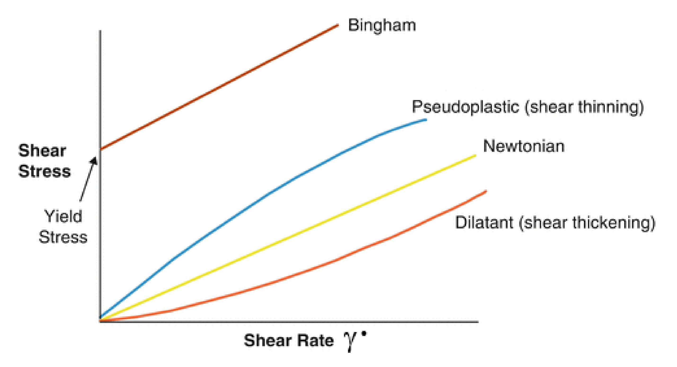
It should be noted, however, that a liquid environment with magnetic particles is generally inhomogeneous and non-isotropic [6,8,9,14,15,16,17]. Due to the magnetic field, the arrangement of the particles changes, causes the liquid to lose its Newtonian behavior, which is characterized by a linear equation between the shear stress and the shear rate. For example, the following applies to an incompressible liquid:

$$\tau ={\eta }_B\mathsf{\gamma },{\eta }_B=\mathrm{const}.$$

(11)

$$\mathrm{where}\tau =\frac{1}{\sqrt{2}}\sqrt{{\sigma }_{ij}{\sigma }_{ij}}=\frac{1}{\sqrt{2}}\sqrt{D_{ij}{D}_{ij}}\mathrm{and}\gamma =\frac{2}{\sqrt{2}}\sqrt{v_{ij}{v}_{ij}}=\frac{2}{\sqrt{2}}\sqrt{d_{ij}{d}_{ij}}$$

(12)

Note that ${\sigma }_{ij} ,v_{ij}$ are symmetric tensors of second order, and $v_{ij}$ is the tensor of deformation velocity.$D_{ij}$ is a deviator of the mechanical stress tensor and $d_{ij}$ is a deviator of deformation velocity.

Figure 1a,b, show the change in the particles’ arrangements and their polarization, caused by the effects of magnetization. It means that the magnetic fluid environment will become inhomogeneous and will have non-isotropic properties. The effects of inhomogeneity and anisotropy will be higher in MR liquids. This will also affect the dependence of shear stress on shear rate, which may have a non-linear character, as can be seen in Figure 2 and Figure 3.

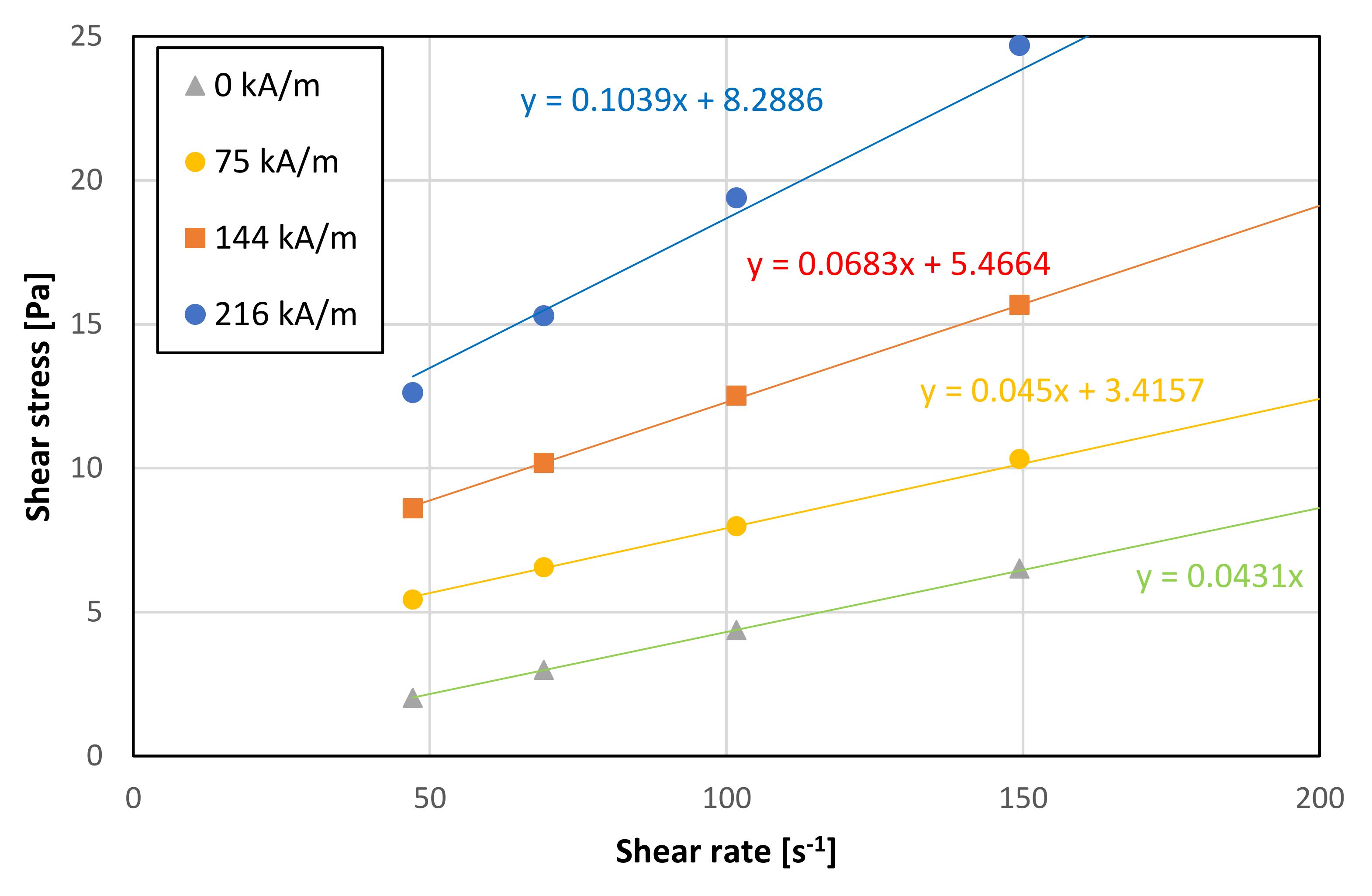
Figure 2 shows the flow curve of the real MR liquid (EMG 900) obtained from the experiments [31]. From this view, it is clear that the diagram can be divided into two parts, which correspond with Bingham’s behavior [6,10], whose mathematical model is as follows:

$$\tau ={\tau }_0+{\eta }_{Bm}\mathsf{\gamma },{\eta }_{Bm}=\mathrm{const}.$$

(13)

where ${\tau }_0$ is the yield stress, and ${\eta }_{Bm}$ is the dynamic viscosity. From the shape of experimentally obtained curves $\tau =\tau \left(\mathsf{\gamma }\right)$ the authors [11] derived a more general constitutive model of a non-Newtonian fluid for 3D problems. Assuming that

$$\tau ={\tau }_0+{\eta }_{Bm}{\gamma }^m,D_{ij}=2\eta \left(d_{ij}{d}_{ij}\right)$$

(14)

By substituting from (14) to (12), it holds that

$${\sigma }_{ij}=D_{ij}=2{\tau }_0\frac{d_{ij}}{\sqrt{2d_{\alpha \beta }{d}_{\alpha \beta }}}+2{\eta }_{Bm}{\left(2d_{ij}{d}_{ij}\right)}^{\frac{m-1}{2}}{d}_{ij}$$

(15)

If we apply this experimentally determined dependence on the magnetic liquid, the values ${\tau }_0$ and ${\eta }_{Bm}$ will depend on magnetic induction $B_i$.

$${\tau }_0={\tau }_0\left(B_i\right),{\eta }_{Bm}={\eta }_{Bm}\left(B_i\right)$$

(16)

In the mentioned case, it should be noted that the relation (16) applies only to the symmetric tensor of irreversible stresses $D_{ij}$ and to the incompressible fluid.

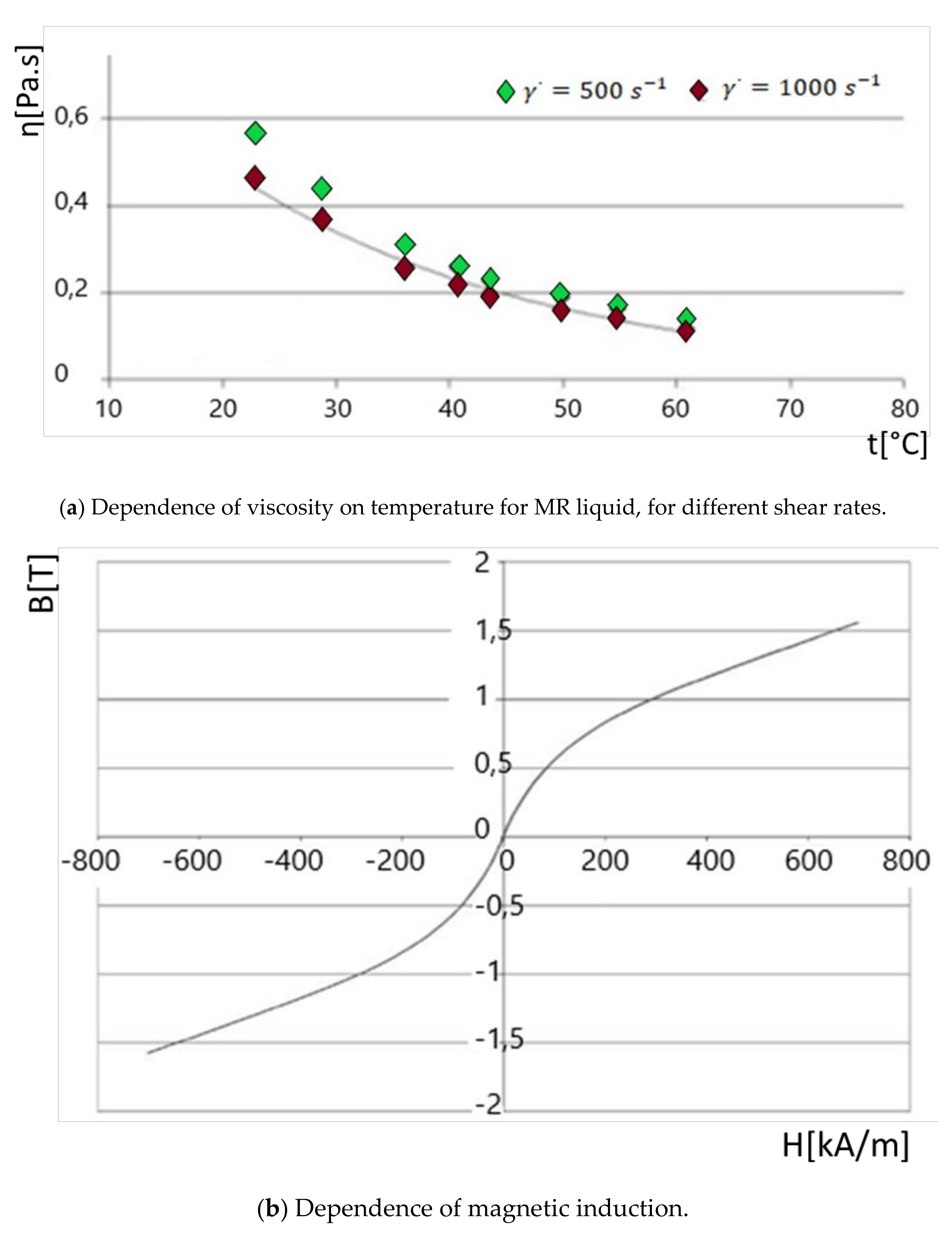
It should be noted, however, that the viscosity of a liquid strongly depends on the temperature, as shown in Figure 4a. The non-linearity of the relationship between the intensity of the magnetic field and the magnetic induction plays an important role in solving the mutual interaction of the liquid and the magnetic field, as shown in Figure 4b.

B. 

Constitutive Model of a Magnetic Liquid with the Effect of Particle Rotation

Within part A, an intuitive constitutive model for a symmetric stress tensor, originally derived for a general non-Newtonian fluid and applied to a magnetic fluid, was presented. Now we present a new constitutive model that considers the asymmetry of the stress tensor, induced by particle rotation, and the effects of surface shear stresses $Y_{ij}{}^S,$ which come as a consequence of the particle–liquid interaction [6,7,8,10,15,16]. When ferromagnetic particles move in a magnetic field, their translational and rotational motions occur at an angular velocity $ῼ$. In this case, stress tensor ${\sigma }_{ij}$ for the incompressible liquid is no longer symmetrical, and the following holds:

$${\sigma }_{ij}=D_{ij}+N_{ij}$$

(17)

$${\mathrm{D}}_{ij}=2\eta {\mathrm{d}}_{ij} ; N_{ij}=2{\eta }_M{\mathrm{d}}_{ij}+2{\eta }_P{\widehat{\omega }}_{ij}$$

(18)

$${\widehat{\omega }}_{ij}=-{ῼ}_{ij}+{\mathsf{\omega }}_{ij}$$

$${\sigma }_{ij}=2\left(\eta +{\eta }_M\right){\mathrm{d}}_{ij}+2{\eta }_P{\widehat{\omega }}_{ij}.$$

(19)

Let us introduce analogously, as in the previous case, that

$$\tau =\frac{1}{\sqrt{2}}\sqrt{{\sigma }_{ij}{\sigma }_{ij}} ; \gamma =\frac{2}{\sqrt{2}}\sqrt{d_{ij}{d}_{ij}}=\sqrt{2d_{ij}{d}_{ij}}$$

(20)

Due to the symmetry of ${\mathrm{d}}_{ij}$ and the antisymmetry of ${\mathsf{\omega }}_{ij}$, it holds that

$$d_{ij}{\widehat{\omega }}_{ij}=0,$$

(21)

and it can be written as follows:

$${\sigma }_{ij}{\sigma }_{ij}=4{\left(\eta +{\eta }_M\right)}^2{d}_{ij}{d}_{ij}+4{\eta }_P^2{\widehat{\omega }}_{ij}{\widehat{\omega }}_{ij}.$$

(22)

Assume that the following rheological model applies to a magnetorheological liquid:

$$\tau ={\tau }_0+{\displaystyle \sum }_{n=1}^N{\eta }_{Bn}{\gamma }^n$$

(23)

$${\tau }^2={\left({\tau }_0+{\displaystyle \sum }_{n=1}^N{\eta }_{Bn}{\gamma }^n\right)}^2=\frac{1}{2}{\sigma }_{ij}{\sigma }_{ij}.$$

(24)

After substitution from (19), it will be as follows:

$${\left({\tau }_0+{\displaystyle \sum }_{n=1}^N{\eta }_{Bn}{\gamma }^n\right)}^2=2{\left(\eta +{\eta }_M\right)}^2{d}_{ij}{d}_{ij}+2{\eta }_P^2{\widehat{\omega }}_{ij}{\widehat{\omega }}_{ij}.$$

(25)

Let us introduce that

$$2{\left(\eta +{\eta }_M\right)}^2{d}_{ij}{d}_{ij}={\kappa }^2{\left({\tau }_0+{\displaystyle \sum }_{n=1}^N{\eta }_{Bn}{\gamma }^n\right)}^2.$$

(26)

After substitution to (25), it will be

$${\left({\tau }_0+{\displaystyle \sum }_{n=1}^N{\eta }_{Bn}{\gamma }^n\right)}^2\left(1-{\kappa }^2\right)=2{\eta }_P^2{\widehat{\omega }}_{ij}{\widehat{\omega }}_{ij}.$$

(27)

From the expressions (26) and (27) it is possible to derive the equations for the unknown values of $\eta +{\eta }_M$ a ${\eta }_P.$ The expression (26) can be written in the following form due to the definition of $\gamma$:

$${\left(\eta +{\eta }_M\right)}^2{\gamma }^2={\kappa }^2{\left({\tau }_0+{\displaystyle \sum }_{n=1}^N{\eta }_{Bn}{\gamma }^n\right)}^2.$$

From it:

$$\eta +{\eta }_M=\frac{\kappa {\tau }_0}{\gamma }+{\displaystyle \sum }_{n=1}^N\kappa {\eta }_{Bn}{\gamma }^{n-1}.$$

(28)

After the substitution from (12), it holds that

$$\eta +{\eta }_M=\frac{\kappa {\tau }_0}{\sqrt{2d_{ij}{d}_{ij}}}+{\displaystyle \sum }_{n=1}^N\kappa {\eta }_{Bn}{\left(2d_{ij}{d}_{ij}\right)}^{\frac{n-1}{2}}.$$

(29)

From the expression (27):

$${\eta }_P=\frac{{\tau }_0\sqrt{\left(1-{\kappa }^2\right)}}{\sqrt{2{\widehat{\omega }}_{kl}{\widehat{\omega }}_{kl}}}+\frac{\sqrt{\left(1-{\kappa }^2\right)}}{\sqrt{2{\widehat{\omega }}_{kl}{\widehat{\omega }}_{kl}}}{\displaystyle \sum }_{n=1}^N{\eta }_{Bn}{\left(\sqrt{2d_{ij}{d}_{ij}}\right)}^n.$$

$${\eta }_P=\frac{{\tau }_0\sqrt{\left(1-{\kappa }^2\right)}}{\sqrt{2{\widehat{\omega }}_{kl}{\widehat{\omega }}_{kl}}}+\sqrt{\left(1-{\kappa }^2\right)}{\displaystyle \sum }_{n=1}^N{\eta }_{Bn}\frac{{\left(\sqrt{2d_{ij}{d}_{ij}}\right)}^n}{\sqrt{2{\widehat{\omega }}_{kl}{\widehat{\omega }}_{kl}}}$$

(30)

The equation for the resulting stress tensor will have the following form:

$$\begin{gathered} {\sigma }_{ij}=2\kappa {\tau }_0\frac{d_{ij}}{\sqrt{2d_{kl}{d}_{kl}}}+2{\displaystyle \sum }_{n=1}^N{2}^{\frac{n-1}{2}}\kappa {\eta }_{Bn}{\left(d_{kl}{d}_{kl}\right)}^{\frac{n-1}{2}}{d}_{ij}+2{\tau }_0\sqrt{1-{\kappa }^2}\frac{{\widehat{\omega }}_{ij}}{\sqrt{2{\widehat{\omega }}_{kl}{\widehat{\omega }}_{kl}}} \\ +2\sqrt{1-{\kappa }^2}{\displaystyle \sum _{n=1}^N}{\eta }_{Bn}\frac{{\left(\sqrt{2d_{ij}{d}_{ij}}\right)}^n}{\sqrt{2{\widehat{\omega }}_{kl}{\widehat{\omega }}_{kl}}}{\widehat{\omega }}_{ij}. \end{gathered}$$

(31)

For N = 1, we obtain a simple relationship between a Bingham liquid and an antisymmetric stress tensor.

$${\sigma }_{ij}=2\kappa {\tau }_0\frac{d_{ij}}{\sqrt{2v_{kl}{v}_{kl}}}+2\kappa {\eta }_{B1}{d}_{ij}+\sqrt{1-{\kappa }^2}(2{\tau }_0\frac{{\widehat{\omega }}_{ij}}{\sqrt{2{\widehat{\omega }}_{kl}{\widehat{\omega }}_{kl}}}+2{\eta }_{B1}\sqrt{\frac{d_{ij}{d}_{ij}}{{\widehat{\omega }}_{kl}{\widehat{\omega }}_{kl}}}{\widehat{\omega }}_{ij})$$

(32)

4. Constitutive Model of a Magnetic Liquid Based on the Entropy Production

The mutual effects of physical fields are characterized by the density of entropy production $\sigma$, which forms the basis for the definition of constitutive equations [1,2,7,10,22,23,24,25]. Its expression depends on the irreversible thermodynamic flows $\left(J^z\right)$ and their corresponding irreversible thermodynamic forces $X^z$:

$$\sigma =J^z X^z$$

(33)

Flows and forces are characterized by a certain tensor dimension. For example [1,10,29,30,32]:

$$J^1 \left(J_i{}^1\right)=\frac{1}{{\tau }_m}\left(M_{oi}-M_i\right)$$

(34)

$J_i{}^1$ is a vector flow of magnetization and

$$X^1\left(X_i{}^1 \right)=\frac{1}{T}\left(H_{oi}-H_i\right)$$

(35)

$X_i{}^1$ is the generalized thermodynamic vector force of the magnetic field intensity, ${\tau }_m$ is the relaxation time, and T is the absolute temperature [7,23]. Symmetric and antisymmetric tensors, as well as vector and scalar variables, can be included in the expression for entropy production density [23] as follows:

$$\sigma =S_{ij}^A{X}_{ij}^A+A_{ij}^B{Z}_{ij}^B+J_i^C{X}_i^C+J^D{X}^D$$

(36)

$S_{ij}$ is the symmetric tensor of the 2nd order, $A_{ij}$ is the antisymmetric generalized thermodynamic force of the tensor of the 2nd order, and $X_{ij}$ is the symmetric generalized thermodynamic force of the tensor of the 2nd order. $A=1,\dots ,M;B=M+1,\dots ,N;C=N+1,\dots ,K;D=K+1,\dots ,H.$

The following relations apply between flows and forces:

$$S_{ij}^A=L_{ijkl}^{Aa}{X}_{kl}^a+L_{ijkl}^{Ab}{Z}_{kl}^b+L_{ijk}^{Ac}{X}_k^c+L_{ij}^{Ad}{X}^d$$

(37)

$$A_{ij}^B=L_{ijkl}^{Ba}{X}_{kl}^a+L_{ijkl}^{Bb}{Z}_{kl}^b+L_{ijk}^{Bc}{X}_k^c+L_{ij}^{Bd}{X}^d$$

(38)

$$J_i^C=L_{ikl}^{Ca}{X}_{kl}^a+L_{ikl}^{Cb}{Z}_{kl}^b+L_{ik}^{Cc}{X}_k^c+L_i^{Cd}{X}^d$$

(39)

$$\begin{gathered} J^D=L_{kl}^{Da}{X}_{kl}^a+L_{kl}^{Db}{Z}_{kl}^b+L_k^{Dc}{X}_k^c+L^{Dd}{X}^d \\ a=1,\dots ,M,b=M+1,\dots ,N;c=N+1,\dots ,K; d=K+1,\dots ,H; \\ L, L_i,L_{ij},L_{ijkl}-\mathrm{transfer}\mathrm{coefficients}(\mathrm{material}\mathrm{constants}\mathrm{for}\mathrm{chosen}\mathrm{i},\mathrm{j},\mathrm{k},\mathrm{l}) \end{gathered}$$

(40)

Alternatively, in the matrix form:

$$\left|\begin{array}{c}\begin{array}{c}{S}_{ij}^A\\ A_{ij}^B\end{array}\\ J_i^C\\ J^D\end{array}\right| = \left|\right|\begin{array}{cccc}{L}_{ijkl}^{Aa}& L_{ijkl}^{Ab}& L_{ijk}^{Ac}& L_{ij}^{Ad}\\ L_{ijkl}^{Ba}& L_{ijkl}^{Bb}& L_{ijk}^{Bc}& L_{ij}^{Bd}\\ L_{ikl}^{Ca}& L_{ikl}^{Cb}& L_{ik}^{Cc} & L_i^{Cd}\\ L_{kl}^{Da}& L_{kl}^{Db} & L_k^{Dc} & L^{Dd}\end{array}\left|\right| · \left|\begin{array}{c}\begin{array}{c}{X}_{kl}^a\\ Z_{kl}^b\end{array}\\ X_k^c\\ X^d\end{array}\right|$$

(41)

Expressions (37)–(41) represent the constitutive equations between irreversible thermodynamic flows and forces. The matrix in expression (41) is formed by the unknown transfer coefficients of a given physical quantity, which are dependent on B in the magnetic field and must be determined from the experiment.

The Curie principle [24] can be used in relation (41). According to the principle, only flows and forces of the same tensor dimension can react together in an isotropic environment. In an isotropic environment, the matrix in expression (41) would be diagonal and the diagonal elements would be scalars. The Onsager conditions of symmetry can also be used for identification [22].

In the previous chapter, the design of constitutive relations was based on experimental experience and in accordance with the experiment, constitutive relations were intuitively designed (32).

The following method of creating constitutive relations is based on the physical laws between irreversible flows and forces (41), which occur after the violation of the state of thermodynamic equilibrium. In this procedure, intuition is replaced with physical laws, using the principles of non-equilibrium thermodynamics [23].

Let us now start from the general relation for the entropy production density $\sigma$(36) [7,23] for a system with n components. The lower indices characterize the tensor character of variables and the upper indices characterize their physical significance. The index convention is used. The index in parentheses is not an addition.

Since magnetic fluids form a multicomponent system, it may be useful to consider the effects of diffusion, chemical reactions, magnetization, and polarization in the production of entropy (36) [7,23]. For the entropy production density $\sigma$ of an electromagnetic fluid, under this assumption, a general relation can be written [7,23]:

$$\begin{gathered} \sigma ={\mathsf{\Pi }}_{ij}^{\left(S\right)}\frac{1}{T}{v}_{ij}^{\left(S\right)}+\frac{1}{3}{\mathsf{\Pi }}_{\alpha \alpha }\frac{1}{T}{v}_{\beta \beta }-J_i^q\frac{1}{T^2}\frac{\partial T}{\partial x_i}-J_i^k\frac{\partial }{\partial x_i}\left(\frac{{\mu }^k}{T}\right)+J_i^E\frac{1}{T}{E}_i-J^l\frac{1}{T}{A}^l+{\mathsf{\Lambda }}_{ij}^{\left(S\right)}\frac{Y_{ij}^{\left(s\right)}}{T}-{\mathsf{\Pi }}_{ij}^{\left(AN\right)}\frac{\left({\mathsf{\Omega }}_{ij}-{\omega }_{ij}\right)}{T} \\ +\frac{1}{3}{\mathsf{\Lambda }}_{\alpha \alpha }\frac{{\mathrm{Y}}_{\alpha \alpha }}{T}+\left(\frac{d{P}_i}{dt}+P_i{v}_{\alpha \alpha }-{\epsilon }_{ij\alpha }{\mathsf{\Omega }}_j{P}_{\alpha }\right)\frac{\left({\mathrm{E}}_{0i}-E_i\right)}{T}+\left(\frac{d{M}_i}{dt}+M_i{v}_{\alpha \alpha }-{\epsilon }_{ij\alpha }{\mathsf{\Omega }}_j{M}_{\alpha }\right)\frac{\left(H_{0i}-H_i\right)}{T} \end{gathered}$$

(42)

$\mathrm{k}=1,\dots \dots ,\mathrm{n}-1,l=1,\dots ,\mathrm{r}.$ Due to the fact that we work in the Cartesian coordinate system, the subscripts take on the values 1,2,3. All indices in expression (42) are summative, except the indices in parentheses.

The following variables are shown in expression (42): ${\mathsf{\Pi }}_{ij}^{\left(S\right)}$—symmetric tensor of mechanical stresses$;\frac{{\delta }_{ij}}{3T}{v}_{ij}^{\left(S\right)}$—spherical tensor of strain rate; $J_i^q$—heat flux; T—absolute temperature; $J_i^k$—diffusion flux; ${\mu }^k$—chemical potential; $J_i^E$—electric flux; $E_i$—electric current intensity; $J^l$—flux (velocity) of chemical reaction; $A^l$—affinity of a chemical reaction; ${\mathsf{\Lambda }}_{ij}^{\left(S\right)}$—symmetric stress tensor induced by the effects of the surface forces of particles; $Y_{ij}^{\left(s\right)}$—symmetric tensor of the generalized thermodynamic forces of the surface forces of a particle; ${\mathsf{\Pi }}_{ij}^{\left(AN\right)}$—antisymmetric tensor of the particle rotation effects; ${\mathsf{\Omega }}_{ij}$—antisymmetric particle rotation tensor; ${\omega }_{ij}$—antisymmetric strain rate tensor; $\frac{1}{3}{\delta }_{ij}{\mathsf{\Lambda }}_{\alpha \alpha }$—spherical tensor of the effects of particle surface forces; $v_{\beta \beta }$—divergence of the velocity vector.

An analogous form of entropy production is given in [7] without the influences of diffusion and chemical reactions. The effects of diffusion and particle separation are partially mentioned in [8,14,15]. The expression for entropy production can be further simplified on the basis of [7,19] according to the following relation for the magnetization vector [7]:

$$\left(\frac{d{M}_i}{dt}+M_i{v}_{\alpha \alpha }-{\epsilon }_{ij\alpha }{\mathsf{\Omega }}_j{M}_{\alpha }\right)=\frac{1}{{\tau }_m}\left(M_{0i}–M_i\right)$$

(43)

5. Magnetic Field

Let us now consider the simpler case of neglecting the effects of temperature, diffusion, chemical reactions, and electric fields. A simpler relation applies to the density of entropy production as follows [7,23]:

$$\begin{gathered} \sigma ={\mathsf{\Pi }}_{ij}^{\left(S\right)}\frac{1}{T}{v}_{ij}^{\left(S\right)}+{\mathsf{\Lambda }}_{ij}^{\left(s\right)}\frac{Y_{ij}^{\left(S\right)}}{T}-{\mathsf{\Pi }}_{ij}^{\left(AN\right)}\frac{\left({\mathsf{\Omega }}_{ij}-{\omega }_{ij}\right)}{T}+\frac{1}{{\tau }_m}\left(M_{oi}-M_i\right)\frac{\left(H_{0i}-H_i\right)}{T} \\ +\frac{1}{3}{\mathsf{\Pi }}_{aa}\frac{1}{T}{v}_{aa}+\frac{1}{3}{\mathsf{\Lambda }}_{\alpha \alpha }\frac{{\mathrm{Y}}_{\alpha \alpha }}{T} \end{gathered}$$

(44)

By comparing (36) and (44), we obtain the following physical meanings of irreversible thermodynamic flows and forces.

Flows:

$$\begin{gathered} S_{ij}^1={\mathsf{\Pi }}_{ij}^{\left(S\right)} S_{ij}^2={\mathsf{\Lambda }}_{ij}^{\left(s\right)} A_{ij}^3={\mathsf{\Pi }}_{ij}^{\left(AN\right)} \\ {J}_i^4=\left(M_{i0}-M_i\right)\frac{1}{{\tau }_m} \\ {J}^5=\frac{1}{3}{\mathsf{\Pi }}_{aa} \\ {J}^6=\frac{1}{3}{\mathsf{\Lambda }}_{\alpha \alpha } \end{gathered}$$

(45)

In the mentioned case:${\widehat{\sigma }}_{ij}=-p{\delta }_{ij}$ +${\mathsf{\Pi }}_{ij}^{\left(S\right)}+{\delta }_{ij}\frac{1}{3}{\mathsf{\Pi }}_{kk}+{\mathsf{\Pi }}_{ij}^{\left(AN\right)}$.

Forces:

$$\begin{gathered} X_{kl}^1=\frac{1}{T} v_{kl}^{\left(S\right)} \\ {X}_{kl}^2=Y_{ij}^{\left(S\right)}=\frac{1}{2T}\left(\frac{\partial {\mathsf{\Omega }}_i}{\partial x_j}+\frac{\partial {\mathsf{\Omega }}_j}{\partial x_i}\right)-\frac{{\delta }_{ij}}{3T}\frac{\partial {\mathsf{\Omega }}_k}{\partial x_k} \\ {Z}_{kl}^3=Y_{ij}^{\left(AN\right)}=\frac{\left({\mathsf{\Omega }}_{ij}-{\omega }_{ij}\right)}{T} \\ {X}_k^4=\frac{1}{T}\left(H_{0k}-H_k\right) \\ {X}^5=\frac{1}{T}{\mathrm{v}}_{ii} \\ {X}^6=\frac{1}{T}\frac{\partial {\mathsf{\Omega }}_k}{\partial x_k} \end{gathered}$$

(46)

The following are shown in expressions (45) and (46): $\mathsf{\Omega } \left({\mathsf{\Omega }}_i\right)$—angular velocity vector of the medium particle$; {\omega }_{ij}$—angular velocity tensor of the liquid$; {\mathsf{\Omega }}_{ij}$—angular velocity tensor of the particle; $v_{ij}$—strain rate tensor; $M\left(M_i\right)$—magnetization vector; $H\left(H_i\right)$—magnetic field intensity vector.

The constitutive equations for the magnetic fluid can thus be expressed by the relations (37)–(40), or by the matrix relation (41). The elements of the matrix depend on the magnetic induction vector B$\left(B_i\right)$ and must be determined from the experiment. The defined constitutive relations can be further simplified since it is expedient to introduce the dependence of the stress tensor on the strain rate tensor into the equilibrium equations for the magnetic fluid. This can be achieved by adjusting the constitutive relations through expressing $X_k^4$ as a function of $X_{kl}^1$ and by using the relationship between the magnetization vector and the magnetic field strength; thus, the dependencies are as follows [1,7,29,30]:

$$\left(M_{oi}-M_i\right)=\mathsf{\chi }\left(\mathrm{H}\right)\left(H_{0i}-H_i\right)$$

(47)

If we mark that

$$\hat{\mathsf{\Lambda }}=\mathsf{\chi }\frac{T}{{\tau }_m}$$

(48)

It can be written that

$$J_i^4{J}_i^4{\left|J_{\left(n\right)}^4\right|}^2={\left(\frac{T}{{\tau }_m}\right)}^2{\mathsf{\chi }}^2{\left|X_{\left(n\right)}^1\right|}^2={\hat{\mathsf{\Lambda }}}^2{X}_i^4{X}_i^4$$

(49)

We now use the experimentally determined dependencies (47) (see Figure 3) to simplify and refine the constitutive relations (37)–(40). We show the methodology for simplification, in which we currently assume only the effects of one flux of magnetization and one flux of the stress deviator. In this case, the entropy production will be in the following form:

$$\sigma ={\mathsf{\Pi }}_{ij}^{\left(S\right)}\frac{1}{T}{v}_{ij}^{\left(S\right)}+\frac{1}{{\tau }_m}\left(M_{oi}-M_i\right)\frac{\left(H_{0i}-H_i\right)}{T}=S_{ij}^1{X}_{ij}^1+J_i^2{X}_i^2$$

(50)

$$S_{ij}^1={\mathsf{\Pi }}_{ij}^{\left(S\right)}=D_{ij},X_{ij}^1=v_{ij}^{\left(S\right)}=d_{ij}$$

(51)

$$J_i^2=\frac{1}{{\tau }_m}\left(M_{oi}-M_i\right), X_i^2=\frac{\left(H_{0i}-H_i\right)}{T}$$

(52)

The production of entropy, expressed in terms of flows and forces, will in this case take the following form:

$$\sigma =S_{ij}^1{X}_{ij}^1+J_i^2{X}_i^2$$

(53)

The following will apply to individual flows:

$$S_{ij}^1=L_{ijkl}^{11}{X}_{kl}^1+L_{ijk}^{12}{X}_k^2$$

(54)

$$J_i^2=L_{ikl}^{21}{X}_{kl}^1+L_{ik}^{22}{X}_k^2$$

(55)

In deriving a simplified dependence between flows and forces, we now use the relation (49), which is justified by the experiment. Let us mark that

$$Q=J_i^2{J}_i^2={\overline{\mathsf{\Lambda }}}^2{X}_i^2{X}_i^2=\left(\underset{U_i}{\underbrace{L_{ikl}^{21}{X}_{kl}^1+L_{ik}^{22}{X}_k^2}}\right)\left(L_{i\kappa \lambda }^{21}{X}_{\kappa \lambda }^1+L_{i\kappa }^{22}{X}_k^2\right)$$

After the decomposition it will be:

$$Q={\overline{\mathsf{\Lambda }}}^2{X}_i^2{X}_i^2=2L_{ikl}^{21}{X}_{kl}^2{L}_{i\kappa }^{22}{X}_{\kappa }^2+L_{ikl}^{21}{X}_{kl}^2{L}_{i\kappa \lambda }^{21}{X}_{\kappa \lambda }^2+L_{ik}^{22}{X}_k^2{L}_{i\kappa }^{22}{X}_{\kappa }^2$$

(56)

In the last expression, let us assume that the relation holds, even in a non-isotropic environment:

$$L_{ik}^{22}=A\overline{\mathsf{\Lambda }}{\delta }_{ik};L_{i\kappa }^{22}=A\overline{\mathsf{\Lambda }}{\delta }_{i\kappa }$$

(57)

Once implemented in the previous equation, it will be

$$L_{ik}^{22}{X}_k^2{L}_{i\kappa }^{22}{X}_{\kappa }^2=A^2{\overline{\mathsf{\Lambda }}}^2{X}_i^2{X}_i^2$$

Next, we put:

$$2L_{ikl}^{21}{X}_{kl}^2=B\overline{\mathsf{\Lambda }}{X}_i^2$$

(58)

We will use the above obtained results to edit other terms as follows:

$$2L_{ikl}^{21}{X}_{kl}^{21}{L}_{i\kappa }^{22}{X}_{\kappa }^2=B\overline{\mathsf{\Lambda }}{X}_i^{2}A\overline{\mathsf{\Lambda }}{\delta }_{i\kappa }{X}_{\kappa }^2$$

$$2L_{ikl}^{21}{X}_{kl}^{21}{L}_{i\kappa }^{22}{X}_{\kappa }^2=AB{\overline{\mathsf{\Lambda }}}^2{X}_i^2{X}_i^2$$

By using (58), we obtain

$$L_{ikl}^{21}{X}_{kl}^2{L}_{i\kappa \lambda }^{21}{X}_{\kappa \lambda }^2=\frac{1}{2}B\overline{\mathsf{\Lambda }}{X}_i^4\frac{1}{2}B\overline{\mathsf{\Lambda }}{X}_i^4={\left(\frac{B}{2}\right)}^2{\overline{\mathsf{\Lambda }}}^2{X}_i^4{X}_i^4$$

$$L_{ikl}^{4a}{X}_{kl}^a{L}_{i\kappa \lambda }^{4\alpha }{X}_{\kappa \lambda }^{\alpha }={\left(\frac{B}{2}\right)}^2{\overline{\mathsf{\Lambda }}}^2{X}_i^4{X}_i^4$$

(59)

We will now focus on the determination of $X_i^2$, to simplify the constitutive Equation (54). From expression (58), it can be deduced that

$$X_i^2=\frac{2}{\overline{\mathsf{\Lambda }}B}{L}_{ikl}^{21}{X}_{kl}^2=\frac{1}{\overline{\mathsf{\Lambda }}}\frac{1}{\frac{B}{2}}{L}_{ikl}^{21}{X}_{kl}^2$$

(60)

From (59), it can be deduced that

$$\frac{B}{2}=\frac{1}{\overline{\mathsf{\Lambda }}\sqrt{X_u^2{X}_u^2}}\sqrt{L_{ikl}^{21}{X}_{kl}^2{L}_{i\kappa \mathsf{\lambda }}^{21}{X}_{\kappa \lambda }^2}$$

(61)

After substituting (59) into the relation, we obtain the following:

$$X_i^2=\frac{\sqrt{X_u^2{X}_u^2}}{\sqrt{L_{ikl}^{21}{X}_{kl}^2{L}_{i\kappa \mathsf{\lambda }}^{21}{X}_{\kappa \lambda }^2}}{L}_{ikl}^{4a}{X}_{kl}^a$$

(62)

With the known $X_i^2 ,$ we can already write a constitutive equation for the stress deviator (54) in the required form:

$$S_{ij}^1=L_{ijkl}^{11}{X}_{kl}^1+L_{ij\kappa }^{12}\frac{\sqrt{X_u^2{X}_u^2}}{\sqrt{L_{mkl}^{21}{X}_{kl}^2{L}_{m\kappa \mathsf{\lambda }}^{21}{X}_{\kappa \lambda }^2}}{L}_{\kappa kl}^{21}{X}_{kl}^2$$

(63)

Let us sign $H_{ijkl}\left(B_{\left(m\right)}\right)=L_{ij\kappa }^{12}{L}_{\kappa kl}^{21}$, $U_{sn\kappa \mathsf{\lambda }}\left(B_{\left(m\right)}\right)=L_{msn}^{21}{L}_{m\kappa \mathsf{\lambda }}^{21}$, then we can write the following:

$$S_{ij}^1=L_{ijkl}^{11}\left(B_{\left(m\right)}\right)X_{kl}^1+\sqrt{X_u^2{X}_u^2}\frac{ H_{ijkl }\left(B_{\left(m\right)}\right)}{\sqrt{U_{sn\kappa \mathsf{\lambda } }\left(B_{\left(m\right)}\right)X_{sn}^2{X}_{\kappa \mathsf{\lambda }}^2}}{X}_{kl}^2$$

(64)

The last expression shows the non-linear form of the constitutive equation of a magnetic liquid, where $D_{ij}$ represents the deviator of the mechanical stress tensor:

$$S_{ij}^1={\mathsf{\Pi }}_{ij}^{\left(S\right)} =D_{ij}$$

$$\sqrt{X_u^2{X}_u^2}=X^1=\frac{1}{T}\left|\left(H_{0i}-H_i\right)\right|$$

$$X_{kl}^2=\frac{1}{T}{d}_{ij}\mathrm{where}{d}_{ij}\mathrm{represents}\mathrm{the}\mathrm{deviator}\mathrm{of}\mathrm{strain}\mathrm{rate}\mathrm{velocity}\mathrm{tensor}\mathrm{of}\mathrm{the}\mathrm{liquid}$$

$$D_{ij}=L_{ijkl}^{11}\left(B_{\left(m\right)}\right)\frac{1}{T}{d}_{ij}+\frac{1}{T}\left|\left(H_{0i}-H_i\right)\right|\frac{ H_{ijkl }\left(B_{\left(m\right)}\right)}{\sqrt{U_{sn\kappa \mathsf{\lambda } }\left(B_{\left(m\right)}\right)d_{sn}{d}_{\kappa \mathsf{\lambda }}}}{d}_{kl}$$

(65)

Expression (65) represents a constitutive equation for an incompressible magnetic fluid, assuming symmetry of the stress tensor. It applies to 3D problems and can be simplified by determining the degree of isotropy of the expressions $H_{ijkl }\left(B_{\left(m\right)}\right), L_{ijkl}^{11}\left(B_{\left(m\right)}\right)$ on the basis of the experiment. From the expression for the magnetic flux $J_{i }^2$, the dependence between the variables A and B can be determined:

$$J_i^2=\hat{\mathsf{\Lambda }}{X}_i^2=L_{ikl}^{21}{X}_{kl}^1+L_{ik}^{22}{X}_k^2$$

(66)

However, it holds (57) and (58) so

$$L_{ikl}^{21}{X}_{kl}^1=\frac{1}{2}B\overline{\mathsf{\Lambda }}{X}_i^2,\hspace{1em}\hspace{1em}{L}_{ik}^{22}=A\overline{\mathsf{\Lambda }}{\delta }_{ik}$$

(67)

After substituting into the previous equation, we obtain an important equation between variables A and B, used to identify phenomenological coefficients:

$$\frac{B}{2}+A=1$$

(68)

It follows from Equations (66) and (67) that, under the given assumptions, even in a non-isotropic environment, the vectors $\left(H_{0i}-H_i\right)$ and $\left(M_{0i}-M_i\right)$ are collinear. For a one-dimensional problem, the constitutive Equation (65) is reduced to the following form:

$$\tau ={\tau }_0+{\displaystyle \sum }_{k=1}^N{\eta }_{Bk}{\gamma }^k$$

(69)

For the Bingham fluid, the terms obtained from the experiment [6,10,31,33] apply to $k=1.$

$$\tau ={\tau }_0\left(B_{\left(n\right)}\right)+{\eta }_{Bk}\left(B_{\left(n\right)}\right) \gamma$$

(70)

We will now use this simplified procedure to specify more general constitutive equations, considering the compressibility of the liquid and the asymmetry of the stress tensor. The starting point will now be the production of entropy (44) and expressions for flows and forces (45), (46). The procedure will be analogous to the previous one. The basis will be the flux of magnetization $J_i^4$.

$$J_i^4=L_{ikl}^{4a}{X}_{kl}^a+L_{ikl}^{4b}{Z}_{kl}^b+L_{ik}^{44}{X}_k^4+L_i^{4d}{X}^d=U_i+L_{ikl}^{4b}{Z}_{kl}^b+L_i^{4d}{X}^d$$

(71)

Let us write that

$$Q=U_i{U}_i=\left(\underset{U_i}{\underbrace{L_{ikl}^{4a}{X}_{kl}^a+L_{ik}^{44}{X}_k^4}}\right)\left(L_{i\kappa \lambda }^{4\alpha }{X}_{\kappa \lambda }^{\alpha }+L_{i\kappa }^{44}{X}_k^4\right)$$

(72)

If we use the analogy with (56), (57), we can write that

$$Q=\left[A^2+AB+{\left(\frac{B}{2}\right)}^2\right]{\overline{\mathsf{\Lambda }}}^2{X}_i^4{X}_i^4$$

(73)

When simplifying the constitutive Equation (71), we proceed analogously with the previous case, using the following dependence between magnetization and the intensity of the magnetic field:

$$\begin{gathered} \overline{\mathsf{\Lambda }}{X}_i^4{X}_i^4=J_i^4{J}_i^4=\left(U_i+L_{ikl}^{4b}{Z}_{kl}^b++L_i^{4d}{X}^d\right)\left(U_i+L_{ikl}^{4s}{Z}_{\kappa \lambda }^s++L_i^{4z}{X}^z\right) \\ \hspace{1em}\hspace{1em}\hspace{1em}\hspace{1em}\hspace{1em}=U^2+2U_i(L_i^{4d}{X}^d+L_{ikl}^{4b}{Z}_{kl}^b)+L_{ikl}^{4b}{Z}_{kl}^b{L}_{i\kappa \lambda }^{4s}{Z}_{\kappa \lambda }^s \\ +2L_{ikl}^{4b}{Z}_{kl}^b{L}_i^{4d}{X}^d\hspace{1em}\hspace{1em}\hspace{1em}\hspace{1em}\hspace{1em}\hspace{1em}\hspace{0.17em} \end{gathered}$$

(74)

The following relations can be derived from expression (74) analogously to the previous case:

$$L_{ik}^{44}=A\overline{\mathsf{\Lambda }}{\delta }_{ik}; 2L_{ikl}^{4a}{X}_{kl}^a=B\overline{\mathsf{\Lambda }}{X}_i^4; L_i^{4\delta }{X}^{\delta }=D\overline{\mathsf{\Lambda }}{X}_i^4; L_{ikl}^{4b}{Z}_{kl}^b=\frac{F}{2}\overline{\mathsf{\Lambda }}{X}_i^4$$

(75)

If we sign that

$$\beta =\sqrt{\left(L_{ikl}^{4a}{X}_{kl}^a+L_{ikl}^{4b}{Z}_{kl}^b\right)\left(L_{i\kappa \lambda }^{4\alpha }{X}_{\kappa \lambda }^{\alpha }+L_{i\kappa \lambda }^{4b}{X}_{\kappa \lambda }^b\right)}$$

(76)

then it is possible to write simplified constitutive relations in the following form:

$$X_i^4=\frac{\left|H_{0n}-H_n\right|}{T\beta }\left(L_{ikl}^{4b}{Z}_{kl}^b+L_{ikl}^{4a}{X}_{kl}^a\right)$$

(77)

$$S_{ij}^A=\left(L_{ijkl}^{Aa}+\frac{\left|H_{0n}-H_n\right|}{T\beta }{L}_{ij\kappa }^{A4}{L}_{\kappa kl}^{4a}\right)X_{kl}^a+\left(L_{ijkl}^{Ab}+\frac{\left|H_{0n}-H_n\right|}{T\beta }{L}_{ij\kappa }^{A4}{L}_{\kappa kl}^{4b}\right)Z_{kl}^b+L_{ij}^{Ad}{X}^d$$

(78)

$$A_{ij}^B=\left(L_{ijkl}^{Ba}+\frac{\left|H_{0n}-H_n\right|}{T\beta }{L}_{ij\kappa }^{B4}{L}_{\kappa kl}^{4a}\right)X_{kl}^a+\left(L_{ijkl}^{Ab}+\frac{\left|H_{0n}-H_n\right|}{T\beta }{L}_{ij\kappa }^{B4}{L}_{\kappa kl}^{4b}\right)Z_{kl}^b+L_{ij}^{Ad}{X}^d$$

(79)

$$J^D=\left(L_{kl}^{Da}+\frac{\left|H_{0n}-H_n\right|}{T\beta }{L}_{\kappa }^{D4}{L}_{\kappa kl}^{4a}\right)X_{kl}^a+\left(L_{kl}^{Db}+\frac{\left|H_{0n}-H_n\right|}{T\beta }{L}_{\kappa }^{D4}{L}_{\kappa kl}^{4b}\right)Z_{kl}^b+L^{Dd}{X}^d$$

(80)

After substituting into (40) it is possible to obtain the relationship between functions A, B, D, F as follows:

$$1=\frac{B}{2}+\frac{F}{2}+A+D$$

(81)

6. Discussion

Figure 2 shows the characteristic of shear stress ${\tau }_{r\phi }$ as a function of shear rate $\gamma =2\frac{\partial v_{\phi }}{\partial r}$, as obtained by the measurement on an Anton Paar MCR 502 rotary viscometer [31]. The flow is characterized here as one-dimensional, where there are no signs of non-isotropy or asymmetry. Mathematical models (15), (32), and (78) are, respectively, reduced here to expression (13), where it is possible to determine the values ${\tau }_0\left(B\right)$ and ${\eta }_{Bm}$ from the diagram in Figure 2. In more general domains, when different types of vortex structures occur, it is necessary to assess the degree of isotropy depending on these structures, and to determine the main directions of isotropy, depending on the shape of the vortex structures and the value of magnetic induction. These circumstances must be considered when modifying the general mathematical model (78)–(80).

The mathematical model is significantly simplified if the experiment shows, for example, that tensors $L_{ijkl}^{Aa},L_{ij\kappa }^{A4}{L}_{\kappa kl}^{4a}, L_{ijkl}^{Ab},L_{ij\kappa }^{A4}, L_{\kappa kl}^{4b}$ are isotropic. If the liquid is incompressible and the degree of asymmetry of the tensors $A_{ij}^B$ is negligible, then expressions (79) and (80) can be neglected, and expressions (32) and (78) can be adjusted to a shape suitable for solving magnetic fluids in 3D space; this is demonstrated as follows:

$${\mathrm{D}}_{ij}=2{\tau }_0\frac{{\mathrm{d}}_{ij}}{\sqrt{2{\mathrm{d}}_{kl}{\mathrm{d}}_{kl}}}+2{\eta }_{Bm}{\mathrm{d}}_{ij}$$

(82)

7. Conclusions

Two approaches to the formation of constitutive equations of magnetic liquid have been presented in this article. The first part presented a methodology using an intuitive approach, based on experimental experience in the fluid flow in rotationally symmetric structures [33,34], where shear rate $\gamma$ is defined as a partial derivative of the velocity in the direction that is perpendicular to jet ($\gamma =\frac{\partial v}{\partial r}$). For 3D problems, a reduced shear rate $\gamma$ was introduced, depending on the deformation rate deviator for the incompressible liquid, determined by the relation (20).

Due to the asymmetry of the mechanical stress tensor—caused by the rotation of ferromagnetic particles and their interaction with the carrier liquid—a new form of constitutive equation for the asymmetric stress tensor in the form (32) was derived on the basis of intuition.

This derivation methodology is limited, in that it is subject to the derivation published in [32,33,34,35,36,37,38,39,40] for a symmetric stress tensor; however, more plausible and accurate equations can be achieved by applying methods of non-equilibrium thermodynamics, respecting the physical state of the problem. Here, it is not necessary to proceed from intuition, but on the contrary, one can proceed from the definition of entropy production, which includes the action of all physical phenomena occurring in a magnetic fluid after a disturbance of the state of thermodynamic equilibrium in a non-isotropic environment. In this way, new general constitutive relations were derived for compressible magnetic fluids, for the symmetrical and anti-symmetrical parts of mechanical stress tensors and spherical stress tensors $\left(\frac{1}{3}{\delta }_{ij}{J}^D\right),$ in the forms of Equations (78)–(80). Identifying these relations, it is necessary to assess the directional side of isotropy and to simplify the constitutive equations in a suitable way, depending on the nature of the solved problem.