Research on Fault Diagnosis of IPMSM for Electric Vehicles Based on Multi-Level Feature Fusion SPP Network

Abstract

At this stage, the fault diagnosis of the embedded permanent magnet synchronous motor (IPMSM) mostly relies on the analysis of related signals when the motor is running. It requires designers to deeply understand the motor drive system and fault characteristic signals, which leads to a high threshold for fault diagnosis. This study proposes an IPMSM fault diagnosis method based on a multi-level feature fusion spatial pyramid pooling (SPP) network, which can directly diagnose motor faults through motor operating current data. This method uses the finite element software Altair Flux to build symmetrical normal motor and demagnetization faulty motor models, as well as an asymmetrical eccentric fault model; conduct a joint simulation with MATLAB-Simulink to obtain fault current data; convert the collected current data into grayscale images, using the data set expansion method to form training and test data sets; and improve the convolutional neural network (CNN) network structure, that is, adding jump connections after each pooling layer and adding a spatial pyramid pooling layer after the last pooling layer to form a new CNN structure. Experimental results show that the new CNN can extract different levels and different scales of motor fault features hidden in the image, and can effectively diagnose different types of IPMSM faults. Compared with the traditional CNN, the new CNN has a higher fault diagnosis accuracy, up to 98.16%, 2.3% higher.

1. Introduction

In recent years, with the increase in the use of electric vehicles, the traffic safety problems caused by them have also increased, and the failure of vehicle motors is an important factor that causes hidden dangers in electric vehicles. Vehicle motor failure will not only cause damage to electric vehicles and threaten the safe operation of electric vehicles, but the additional downtime caused by motor failures will also cause huge economic losses [1]. IPMSM has the advantages of high efficiency, high power density, high reliability, and convenient maintenance, and is widely used in electric vehicles [2]. Therefore, the development of IPMSM fault diagnosis and monitoring technology to realize fault warning has an important application value.

Based on the relevant literature on motor fault diagnosis at home and abroad, the current motor fault diagnosis methods can be mainly summarized into three categories: model-based, data-driven, and knowledge-based methods [3]. Among them, the model-based method needs to establish, first, the mathematical model of the faulty motor. The modeling methods can be based on the classic state estimation or process parameter estimation method, on the equivalent magnetic circuit method, on the winding function and the improved winding function method [4], on the finite element method, and so on [5,6]. The basis of this method is an accurate mathematical model of the motor, and a fault analysis is performed on the basis of the model. The advantage is that it goes deep into the nature of motor operation, but the disadvantage is that it must rely on an accurate mathematical model of the motor. However, the mathematical model of the motor is affected by various factors, such as the non-linearity of the iron core, the working environment, etc., so that it is difficult to establish. Therefore, the accuracy of their diagnosis results is not high, and the realization of the diagnosis technology is also difficult. The second method is data-driven, avoiding the problem of the mathematical model of the diagnostic object to a certain extent. At present, the methods that have been successfully applied to motor fault diagnosis based on data driving include: (1) the spectrum analysis method of stator current [7], (2) the park vector method [8], (3) the instantaneous power decomposition method [9], (4) the wavelet analysis method [10], (5) the high frequency signal injection method [11], (6) and a method based on vibration signal spectrum analysis [12]. However, to adopt these methods, the designer needs to have a wealth of prior knowledge in signal processing and expertise in fault diagnosis. The third method is a knowledge-based method, which has been widely used over the years, mainly due to the development of various artificial intelligence algorithms in various fields, such as aircraft [13,14], transportation [15], and agriculture [16] and many other fields. At present, knowledge-based motor fault diagnosis methods mainly include the following: (1) diagnosis methods based on fuzzy logic; (2) fault diagnosis methods based on expert systems; (3) diagnosis methods based on artificial neural networks [17]. Compared with expert systems, artificial neural networks do not need to construct a knowledge base and an inference engine. They only need a large number of examples of training and to fix the parameters of the neural network to complete the fault diagnosis of the motor.

In recent years, many mechanical faults have been diagnosed based on vibration signal analysis using artificial neural networks and support vector machines [18]. The literature [19,20,21] proposed DTS-CNN, adaptive DCNN and TICNN, respectively, which are realized by processing motor vibration signals. One study [22] uses CNN to realize the fault classification of the rotating machinery, including bearings with mildly insufficient lubrication, bearings with insufficient lubrication and damage to the outer ring of the bearing. Another study [23] inputs the FFT amplitude of the motor current and the detailed parameters of the wavelet transform into the one-dimensional CNN for learning, which is used to diagnose PMSM demagnetization faults and bearing faults. Tamilselvan and Wang proposed a new multi-sensor health diagnosis method in [24]. This method uses a deep belief network based on a restricted Boltzmann machine and trains each layer as a deep network structure, one by one. Although the above-mentioned intelligent diagnosis method based on vibration signal analysis can achieve good results in fault diagnosis, it is a complicated process to eliminate background noise. In addition, vibration measurement is also affected by the installation position of the sensor, and installing the sensor on the motor will also bring additional costs. Electric vehicles are prone to bumps and jitters during driving, which will affect the sensors that measure vibration signals, thereby affecting the reliability of motor fault diagnosis. Therefore, this study proposes an IPMSM fault diagnosis method based entirely on the time-domain signal of the motor stator current to monitor the faults of the IPMSM under the working conditions of electric vehicles.

The main contributions of this article are:

(1) The current signal is used for motor fault diagnosis. In terms of cost, there is no need to add sensors other than the motor drive system, which reduces the use of components. In terms of diagnostic performance, it can reduce the influence of background noise and other mechanical interference, and make the diagnostic method more reliable.

(2) The neural network is applied to the fault diagnosis of IPMSM. Compared with the traditional fault diagnosis method, this method does not need to rely on precise motor mathematical models, nor does it require researchers to have a rich prior knowledge and professional knowledge.

(3) In the traditional convolutional neural network, jump connection and spatial pyramid pooling (SPP) are added to enhance the feature extraction ability of the model and improve the accuracy of motor fault diagnosis.

The rest of this article is arranged as follows: Section 2 introduces the construction of symmetric and asymmetric IPMSM models on the finite element software Altair Flux, and a co-simulation with MATLAB; Section 3 compares several image conversion methods to convert the current signal into a grayscale image to obtain data; Section 4 describes the neural network architecture used in this article; Section 5 mainly introduces the training process and performance analysis of the built neural network; 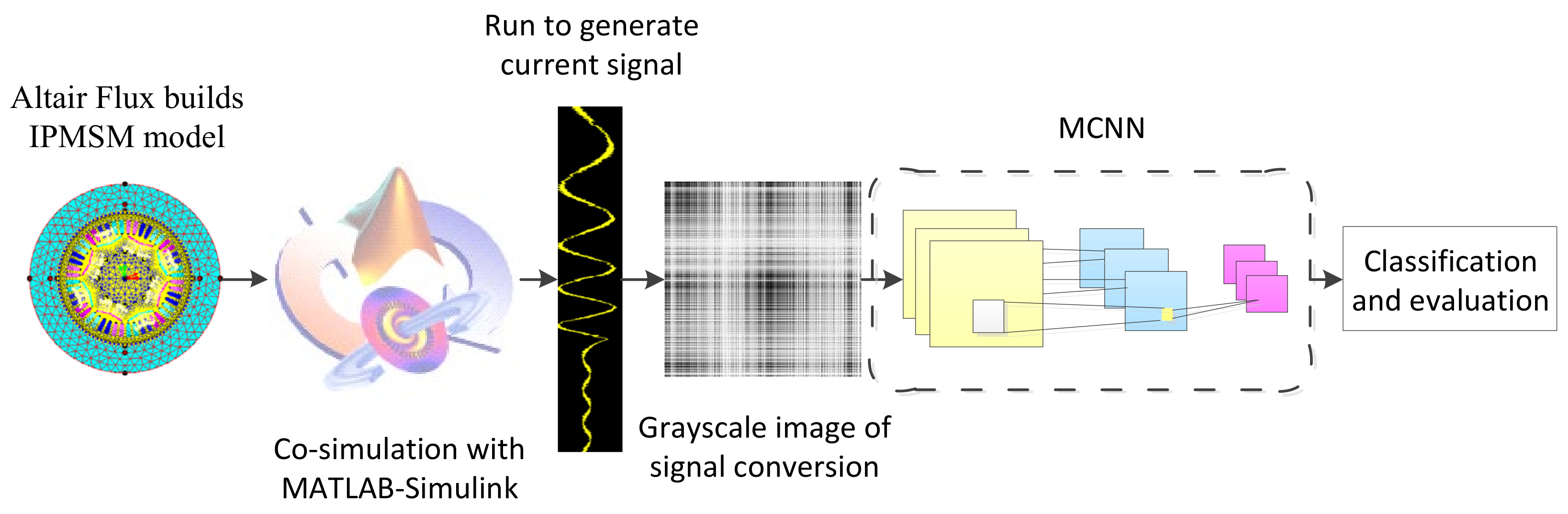Section 6 presents the conclusions. The overall flow chart of the entire experiment is shown in Figure 1.

2. Establish a Faulty IPMSM Simulation System Based on Altair Flux and MATLAB

Altair Flux is a finite element modeling software, which is normally used for the modeling and simulation of magnetic, electrical, and thermal fields [25]. Flux is widely used in the field of motor design, in DC motors, induction motors, synchronous motors, etc. In addition, Flux’s manager also integrates a material manager, a unit manager, and some common system options. The process of using Flux to build a motor model can be divided into the following four parts:

(1)

Establish a geometric model of the motor;

(2)

Set the physical properties, including material setting, external circuit design, and mechanical property setting;

(3)

Set the solution parameters and solve the model;

(4)

To process the solution results, Flux saves a corresponding file for each step of the solution state. To obtain the solution results of each parameter, you need to perform “post-processing” to visualize or save the results.

Motor faults can be divided into three main categories [26]: electrical faults, mechanical faults, and magnetic faults. In this study, the eccentric fault in the mechanical fault category and the demagnetization fault in the magnetic fault category are taken as examples, and the neural network is used to diagnose these two faults.

Taking into account the structural characteristics of the electric vehicle machine, this article refers to the geometric parameters of the hybrid energy vehicle motor in the Flux official tutorial, and redesigns the electrical, mechanical, and permanent magnet structure of the motor on the basis of the original parameters. In this study, an 8-pole, 48-slot IPMSM geometric model is established, and its size specifications are shown in

Table 1. Geometric parameters of the IPMSM model.

Stator Design Parameters		Rotor Design Parameters
Number of stator slots	48 mm	Number of poles	8
Notch width	2 mm	Embedded magnet type	V
Tooth depth	30 mm	Rotor shaft radius	56 mm
Tooth width	6.5 mm	Rotor outer diameter	92 mm
Number of phases	3	Permanent magnet thickness	5 mm
Winding shape	Single-pole double-layer winding	Magnet width	54 mm
Outer diameter of stator	141 mm	Permanent magnet pole arc	140°

.

2.1. Modeling the Static Eccentric Fault Motor

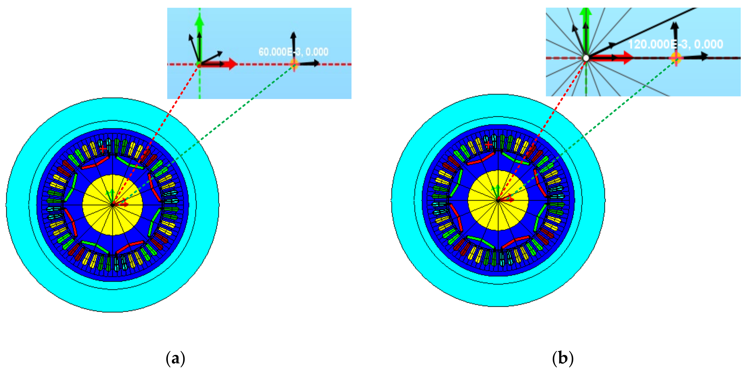
Because the motor with eccentric fault is an asymmetric structure, the complete geometric structure of the motor body needs to be designed when the motor with eccentric fault is built in Flux. Therefore, when establishing the IPMSM geometric model, you need to select “With Eccentricity” at the air gap setting. The rotation center of the IPMSM rotor can be set in the mechanical properties to further determine the type of eccentricity fault of the IPMSM. By changing the center coordinates of the motor stator, this study establishes IPMSM with 10% and 20% static eccentricity faults.

As shown in Figure 2a, the stator center coordinates Or and the rotor axis coordinates Os of the 10% eccentric IPMSM are set to (0.06,0) and (0,0), respectively, so that |OsOr| is 0.06 mm (uniform air, the gap length is 0.6 mm); Figure 2b shows that the stator and rotor axis of a 20% eccentric IPMSM are set to (0.12,0) and (0.0), respectively, so that |OsOr| is 0.12 mm. Then, in the mechanical properties, set the rotor rotation center to (0.0) so that the rotor rotation center and the rotor axis coincide.

2.2. Demagnetization Fault IPMSM Modeling

The neodymium boron (NdFeB) permanent magnet is currently the material of choice for permanent magnet synchronous motors. Compared with other types of magnets, it has a better energy density and a lower cost, but its magnetization will be affected by the working conditions. After demagnetization occurs, it is irreversible and will increase with time. IPMSM for electric vehicles often works in a high-temperature environment with a small space, so demagnetization is prone to occur. The built-in installation method makes the permanent magnets less susceptible to vehicle shaking and damage. Therefore, in the working condition of electric vehicles, the demagnetization of permanent magnets is mostly uniform demagnetization [27]. This study also mainly analyzes the uniform demagnetization failure of IPMSM.

In Flux, NdFeB permanent magnets can be defined by “Linear magnetic described by the Br module”. Set the value in “Remanent flux density” to define the remanence of permanent magnet materials; set “Relative permeability” to define the slope of the magnetic curve. In order to establish an IPMSM model for permanent magnets with different degrees of demagnetization failures on pole pairs, this study defines three magnetic curves, which are the magnetic curves of normal, 25%, and 50% demagnetized materials.

As shown in Figure 3, the remanence Br of the normal permanent magnet is set to 1.2 T, and the permeability is set to 1.05. The remanence Br of 25% and 50% demagnetization permanent magnets is set at 0.9 T and 0.6 T, respectively, while the permeability remains unchanged, and the coercivity increases correspondingly. Figure 4a–c show the magnetic density distribution diagrams of the normal, demagnetized, 25%, and 50% demagnetized IPMSM permanent magnets. The magnetic density distribution of the permanent magnet in the left column of the picture shows that the degree of demagnetization is deeper when the magnetic density distribution becomes sparser.

2.3. Design of the IPMSM Coupling Circuit

In addition to the geometric model, the coupling circuit between the external power supply circuit and the electrical components in the motor body is also an important part of IPMSM. Figure 5 shows the circuit diagram of the coupling circuit embedded in the motor body. The IPMSM winding connection shape adopts a Y connection, VA, VB, VC, and the internal resistance R constitute a three-phase controllable power supply, which can be controlled by an external power supply circuit to input the voltage vector of the motor; AC Coil P&N represents the two parts of the single-phase winding. The direction of one part needs to be set to be opposite to the current, and the number of turns of each winding is 104.

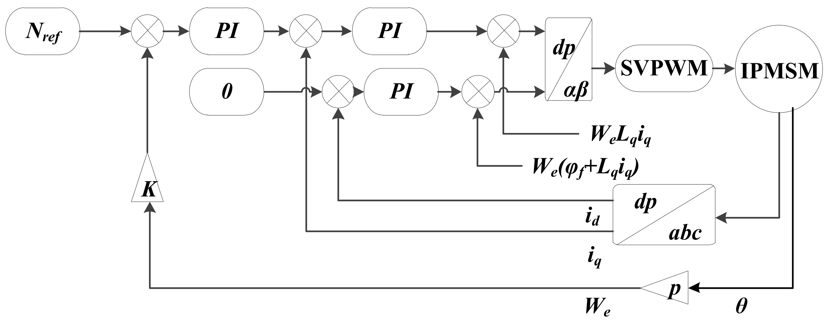
2.4. Co-Simulation

In this study, combining the accuracy of the finite element model and the convenience of the MATLAB control algorithm, the IPMSM finite element model established by Altair Flux is embedded into the vector control system in the MATLAB-Simulink environment, and then a real-time simulation is performed in the loop. The current strategy in the vector control system uses i_d = 0, and the space vector pulse width modulation (SVPWM) algorithm is used to modulate the motor supply voltage vector. The control system block diagram is shown in Figure 6. Figure 7 shows the IPMSM finite element model-in-the-loop simulation system of Altair Flux and MATLAB-Simulink co-simulation.

The IPMSM model and the normal IPMSM model of the four fault categories are jointly simulated. There are eight operating processes for each motor model during the simulation, as shown in

Table 2. The running process of each model.

Load/N.m	Speed/rpm
0	0–2000	0–3000	0–4000	0–5000
10	0–2000	0–3000	0–4000	0–5000

.

Figure 8 shows the simulation results of normal, demagnetized 25%, and 50% demagnetized IPMSM at a given speed of 4000 rpm and a load of 0N.m. Figure 8a–c are the three-phase current simulation results of the three types of motors. It can be seen that the demagnetization fault has a certain effect on the current. The greater the degree of demagnetization, the longer the adjustment time required for the phase current to enter the steady state. Figure 8d is a comparison of the speeds of three types of motors. It can be seen that the speed of the motors with demagnetization faults needs more time to stabilize than that of the normal motors. Figure 8e is the comparison of the electromagnetic torque. From the directly distinguishable characteristics, the dynamic process becomes longer with the increase of the fault intensity, just like the influence on current and speed; and the greater the degree of demagnetization, the smaller the electromagnetic torque. It can be seen that the demagnetization failure reduces the output torque of the motor, which is equivalent to increasing the motor load, which increases the time from the start of the motor to the stable speed.

Figure 9 shows the simulation results of a normal IPMSM with 10% eccentricity and 20% eccentricity at a given speed of 4000 rpm and a load of 0N.m. Figure 9a–c are the simulation results of three-phase stator currents of three types of motors, Figure 9d is the comparison of three types of motor speed, and Figure 9e is the comparison of the electromagnetic torque. From Figure 9a–e, it can be seen that the pure static eccentricity fault has very little effect on the motor, and the three-phase current, speed, and electromagnetic torque trend of the normal, eccentric 10%, and eccentric 20% IPMSM stators are basically the same.

3. Convert IPMSM Operating Current Data into Images

Because convolutional networks are not good at processing high-frequency continuous signals such as motor current, it is difficult to directly extract fault features from the IPMSM stator current time-domain signal. In order to use the convolutional network to extract useful features from the time-domain signal of the motor current signal, this study converts the current signal into a picture, so that the motor signal can adapt to the mechanism of the convolutional network for processing the signal. An image data is a matrix composed of pixel values from 0 to 255. The conversion of data into an image is essentially a process of converting a data sequence into a multi-dimensional matrix. The methods of converting time series data into images in the current literature can be divided into three categories, respectively summarized as the image conversion methods of arrangement, color filling, and coordinate mapping.

3.1. Conversion Method Based on Data Sorting

The image conversion method based on data arrangement directly samples the continuous data and arranges them into a matrix, and then converts the values in the matrix into pixel values in the image through a layer of mapping relationship. Figure 10 shows this conversion process. The literature [28] adopted this transformation method. However, this conversion method requires a long sample data. If the motor status changes too fast, forming an image requires the motor to run for several cycles.

3.2. Image Conversion Method Based on Color Filling

The color-filling-based image conversion method is used to map the sample data to a specified color gamut according to a function. The color-filling method is essentially a linear transformation, and this process can be represented by a uniform distribution:

$$\left\{\begin{array}{cc}P\left(p_{x,y}\right)=\frac{1}{b-a},& a<p_{x,y}<b\\ P\left(p_{x,y}\right)=0,& else\end{array}\right.$$

(1)

In the formula, $p_{x,y}$ represents the pixel in the x-th row and y-th column of the image matrix; a and b represent the maximum and minimum values, respectively, in the original sample; in this uniform distribution, probability $P\left(p_{x,y}\right)$ corresponds to the weight of the color bar. On study [29] visualizes the variable changes in the semiconductor production process in this way, links key variables with defective semiconductors, and finds defective semiconductors by observing key variables. However, this linear mapping method may not be able to express the characteristics of the original data, because there is no logical relationship between the pixel value and the data between the selected color bars.

3.3. Image Conversion Method Based on Coordinate Transformation

On study [30] proposed a method for transforming the characteristic amplitude and phase of the frequency response into polar coordinates, so that each point in the polar coordinates corresponds to the phase and amplitude of the frequency response characteristic at a specific frequency, which makes the frequency response’s characteristic distribution more recognizable. This essentially transforms the turn-to-turn short circuit characteristics of a transformer to another coordinate system. This method is a great improvement for the human eye, but for the machine, this method still has the problem of mapping logic that appears in the coloring method.

3.4. Image Conversion Method Based on Autocorrelation Matrix

There are some shortcomings in the three above-mentioned image conversion methods (excessively long original data are required; there are logic problems, etc.). This article abandons the idea of converting data into three-channel images and converts the original data into a grayscale image with only one channel, so that the original data and the image maintain a rigorous mapping logic relationship. In principal component analysis (PCA), the autocorrelation matrix of a signal is normally used for feature decomposition [31]; in the ESPRIT algorithm, which is often used in radar signal analysis, the autocorrelation matrix and mutual correlation matrix of the array signal are also used. The correlation matrix is used to estimate the parameters of the array signal, such as phase and frequency. Inspired by the PCA and ESPRIT algorithms, this study converts the motor current signal into a two-dimensional matrix by obtaining its autocorrelation matrix. This is essentially a method of upscaling data, and high-dimensional features often contain more data features. In addition, the data sample value scattered into the gray value range can be regarded as a probability problem. Like the image conversion method based on color filling, the weight value of the original data converted to the color area is regarded as a uniform distribution. According to the law of large numbers, as long as the data sample size is large enough, these data will obey the Gaussian distribution. For this reason, this study sets the mapping function of data scattered to the gray value range as a one-dimensional Gaussian distribution function, as shown in Equation (6). Figure 11 shows the flow of image conversion based on the autocorrelation matrix.

$$f\left(x_{ij}\right)=255\times \frac{1}{\sqrt{2\pi \sigma }}{e}^{\frac{{\left(x_{ij}-u\right)}^2}{{\sigma }^2}}$$

(2)

In the formula, $x_{ij}$ represents the element in the i-th row and j-th column in the autocorrelation matrix; µ is the mean value of the original data; σ² is the variance of the original data.

Compared with the image conversion method based on the arrangement, the image conversion method based on the signal autocorrelation matrix requires less original data and higher timeliness. Compared with the color-filling conversion method, the image conversion method based on the autocorrelation matrix makes the original data and the image pixel value have a complete mapping relationship, and the logic is more rigorous.

3.5. Data Set

In this study, the current data in the joint simulations are converted into grayscale images from the time corresponding to the speed of 50 rpm. First, take a sample of 500 data every 30 data points for the phase current. The way to intercept the data is shown in Figure 12:

Then, use the above-mentioned image conversion method based on the autocorrelation matrix to convert each sample into a grayscale image. After converting the current data of five kinds of motors in eight kinds of operation processes (refer to Table 2) into grayscale images, part of the images are randomly selected and rotated by 90 degrees through the method of data expansion, and an image data set including five categories (25% demagnetization, 50% demagnetization, normal, 10% static eccentricity and 20% static eccentricity). It contains 50,000 samples, and the number of samples for each type of motor is 10,000. To verify the reliability of the algorithm, this study randomly and uniformly selects 20% of the 50,000 samples as the model test set, and each category contains 2000 samples. Due to space limitations, Figure 13 and Figure 14 show the grayscale images after a partial fault current data conversion.

It can be seen from Figure 13 and Figure 14 that during the increase of the motor speed, the electromagnetic torque needs to be increased, and the current amplitude is larger when the speed is stable. Therefore, most of the image during the ascent process has low gray values, and more areas of the gray image appear black; most of the images during the stabilization process have higher gray values, and more areas of the gray image appear white. In the process of data preprocessing, because CNN training generally requires a large data set, the method of reading photos one by one is a waste of CPU and GPU computing resources. In this study, in the TensorFlow framework system, the sample image is made into a TFRecord format file, so that the image is compressed into a binary code. During training, the binary code is decoded into a picture and input into the convolutional network model for training.

4. Network Structure

4.1. Multi-Level Feature Fusion

The traditional neural network model only considers the information of the previous layer for the input of each layer and does not consider the information input of other layers globally. The original design intention of the residual network (ResNet) uses jump connections to solve the problem of gradient disappearance in the case of deep network layers, and at the same time helps the back propagation of the gradient and speed up the training process. In the process of forward transmission, as the number of layers deepens, the image information contained in the Feature Map will decrease layer by layer, and the addition of ResNet direct mapping ensures that the network of layer l + 1 must contain more images than the information on layer l. One study [32] improved the VSDR and DRRN models by jumping connections, but directly connecting the data of different layers to obtain more features will also cause a greater occupation of computer resources and reduce the training speed of the network. Referring to the Resnet model, the jump connection network designed in this study firstly carries out the maximum pooling of different layers of data at different scales, then carries out jump connection, and then carries out data fusion with the last pool layer as the input of the full connection layer. It can effectively extract features of different levels by fusing data with lower and higher abstractions [33], and will not cause too much influence on the training speed. Figure 15 shows the jump connection process.

4.2. Spatial Pyramid Pooling Network

The Spatial Pyramid Pooling Layer (SPP) is a special pooling layer proposed by SPPNet [34] to solve the fixed output problem of the fully connected layer. As the fully connected layer of the classifier, it is necessary to map the various features learned by the convolutional layer to the label and to fix the size of the feature map [35]. Before the fully connected layer, SPPNet uses pooling structures with different sizes to extract features from feature maps of any size by adding spatial pyramids, and the resulting feature maps have a fixed size, and then connect to the fully connected layer. One study [36] proposed a convolutional neural network based on spatial pyramid pooling to classify and diagnose seven types of motor faults, which effectively improved the accuracy of the network model. Another [37] pointed out that SPPNet not only obtains better results, but also shares the computational cost between SPP layers and improves the detection efficiency. Therefore, this study designs a spatial pyramid pooling layer placed before the fully connected layer. The data before the full connection is multi-level, pooled through four pooling structures, and multi-scale features are extracted and sent to the fully connected layer. It can effectively improve the convergence speed and accuracy of the network [38]. Figure 16 shows the SPP pooling process in this study, where the input data size is 6 × 6, the four pooling layers are 1 × 1, 2 × 2, 3 × 3, 6 × 6, and the final output size is 1 × 50 data.

4.3. MCNN Network Structure

Based on the traditional CNN model, this study designs an eight-layer convolutional neural network MCNN with SPP and jump connection, which includes six convolution layers and two full connection layers, and Max pool is selected for all the pooling layers to extract the feature texture of the image. A spatial pyramid is introduced after the sixth pooling layer to facilitate the extraction of different scale features of the data; the first five pooling layers are separately pooled and then jumped and connected to extract data features with different levels of abstraction, and then finally combined with the data after SPP Data Fusion. The MCNN network model has a total of 714,053 training parameters, and the network structure is shown in Figure 17:

5. Training and Performance Analysis

5.1. Experimental Environment

The simulations were accomplished on Python 3.7 using TensorFlow 2.0. The network training platform is based on the high-performance server Sugon W580-G20, in which Tesla P4 is selected as GPU, CUDA version is 10.0, and CUDNN version is 7.6.5. The specific platform environment configuration was listed in

Table 3. Experimental environment configuration.

Platform	Related Information
CPU	Intel(R) Xeon(R) CPU E5-2620
GPU	Tesla P4
Operating system	Windows 7 64 bit
CUDA version	10.0
CUDNN version	7.6.5
TensorFlow version	2.0.0
Python version	3.7.0

.

5.2. Training Parameter Settings

In this study, the step-like attenuation learning rate is selected. In the training process, according to the attenuation coefficient, it is reduced once every five rounds. The initial learning rate is large, and can converge quickly and save training time. The later learning rate is small to avoid parameters missing the optimal solution. The attenuation learning rate function used in this study is:

$$l=l_0\times {\alpha }^{\left[\frac{n}{k}\right]}$$

(3)

In the formula, $l_0$ is the initial learning rate; $\alpha$ is the attenuation coefficient; n is the current iteration round number; k is a constant, which can control the rate of change of the learning rate; $\left[\frac{n}{k}\right]$ represents the rounding of $\frac{n}{k}$; $l$ is the learning rate of the n-th generation of neural network training.

After many experiments, it is found that the convergence is faster when the learning rate is 0.01 at the beginning, and the optimal solution can be better obtained when the learning rate is about 0.001 in the later period, so the learning rate interval should be between 0.001 and 0.01. The initial learning rate is set to 0.01, the attenuation coefficient is set to 0.85, k is set to 5, the training is performed for 30 rounds, and the training results can be obtained faster and better. The graph of the stepwise decay learning rate function is shown in Figure 18:

The loss function selected in this study is the cross entropy loss function, which is used to evaluate the difference between the probability distribution obtained by the current training and the real distribution. It depicts the distance between the actual output and the expected output, that is, the smaller the cross entropy, the closer the two probability distributions. Its definition is as follows:

$$C=-\frac{1}{n}{\displaystyle \sum _x\left[y\ln a+\left(1-y\right)\ln \left(1-a\right)\right]}$$

(4)

where x represents the sample, n represents the total number of samples, y represents the desired output, and a represents the actual output of the neuron. Other model parameters are shown in

Table 4. MCNN network model parameters.

Network Parameters	Value
MCNN layers	8
Epoch	30
Loss function	Categorcal_crossentropy
Optimizer	Adagrad
Activation function	Relu
Initial learning rate	0.01
Learning rate decay rate	0.85
Number of convolution kernels per layer	64
Batch size	16

:

In the above table, the selection of the parameter values of the convolution kernel and pooling kernel of the MCNN has been given in Figure 11.

5.3. Evaluation Index

To make the experimental results more convincing, this article compares multiple evaluation indicators, including accuracy, Macro-precision, Macro-recall, and Macro-F1. For the two-category problem, the input and output can be divided into the following four situations, as shown in

Table 5. Two-class confusion matrix.

	Label Is Positive	Label Is Negative
Prediction is a positive sample	TP	FP
Prediction is a negative sample	FN	TN

:

In the table, TP indicates that the prediction is positive and the actual is positive; FP indicates that the prediction is positive and the actual is negative; TN indicates that the prediction is negative and the actual is negative; FN indicates that the prediction is negative and the actual is positive. Macro-precision, Macro-recall, and Macro-F1 can be obtained by averaging Precision, Recall, and F1-score of each category after considering multiple classification problems as multiple binary problems. Precision is the ratio of the number of samples correctly retrieved as a positive class to the total number of samples retrieved as a positive class, Recall is the ratio of the number of samples correctly retrieved as a positive class to the number of samples that should be retrieved as a positive class, and F1-score is the harmonic average of Precision and Recall, and is a comprehensive index of precision and recall. The formulas of Precision, Recall, and F1-score are as follows:

$$Precision=\frac{TP}{TP+FP}$$

(5)

$$Recall=\frac{TP}{TP+FN}$$

(6)

$$F1-score=\frac{2}{P^{-1}+R^{-1}}=\frac{2PR}{P+R}$$

(7)

Based on the above formula, we get the Accuracy, Macro-Precision, Macro-Recall, and Macro-F1 formulas for multiple classifications [39]:

$$n\_correct=T{P}_0+T{P}_1+\cdots +T{P}_{N-1}$$

(8)

$$Accuracy=\frac{n\_correct}{n\_total}$$

(9)

$$Macro-Precision=\left(\frac{T{P}_0}{T{P}_0+F{P}_0}+\frac{T{P}_1}{T{P}_1+F{P}_1}+\cdots \frac{T{P}_{N-1}}{T{P}_{N-1}+F{P}_{N-1}}\right)\times \frac{1}{N}$$

(10)

$$Macro-Recall=\left(\frac{T{P}_0}{T{P}_0+F{N}_0}+\frac{T{P}_1}{T{P}_1+F{N}_1}+\cdots \frac{T{P}_{N-1}}{T{P}_{N-1}+F{N}_{N-1}}\right)\times \frac{1}{N}$$

(11)

$$Macro-F1=\left(\frac{2P_0{R}_0}{P_0+R_0}+\frac{2P_1{R}_1}{P_1+R_1}+\cdots \frac{2P_{N-1}{R}_{N-1}}{P_{N-1}+R_{N-1}}\right)\times \frac{1}{N}$$

(12)

where N represents the number of categories, $n\_correct$ represents the total number of samples, and P and R represent the previous Precision and Recall, respectively.

5.4. Performance Analysis

The traditional convolutional neural network model (hereafter denoted by CNN) only uses jump connection CNN (hereafter denoted by JCNN), spatial pyramid pooling CNN (hereafter denoted by SCNN), and the network model MCNN designed in this article’s comparative analysis. The basic parameters of the four network models are shown in Table 4. They are trained for 30 rounds under the same data set, and their test accuracy and loss in each round are shown in Figure 19. Among them, CNN val_acc, JCNN val_acc, SCNN val_acc, and MCNN val_acc are the test accuracy curves of CNN, JCNN, SCNN, and MCNN, respectively. CNN val_loss, JCNN val_loss, SCNN val_loss, and MCNN val_loss are the test loss curves of CNN, JCNN, SCNN, and MCNN, respectively.

It can be seen from Figure 19 that the test accuracy of JCNN and SCNN is significantly higher than that of CNN, and the test loss is significantly lower than that of CNN. The test accuracy of MCNN is higher than that of JCNN and SCNN, and the test loss is lower than that of JCNN and SCNN. In addition to using accuracy as the evaluation index of the network model, this study also selects Macro-Precision, Macro-Recall, and Macro-F1 as the evaluation index. The diagnosis and evaluation status of CNN models with different structures was listed in

Table 6. Evaluation indicators of CNN models with different structures.

Model	Accuracy	Macro-Precision	Macro-Recall	Macro-F1
MCNN	98.21%	98.22%	98.21%	98.21%
SCNN	97.25%	97.26%	97.25%	97.25%
JCNN	97.36%	97.37%	97.36%	97.36%
CNN	95.86%	95.87%	95.86%	95.86%

.

It can be seen from Table 6 that the CNN test accuracy rate is 95.86%, and the JCNN test accuracy rate is 97.36%, which is 1.5% higher than the traditional CNN. This shows that jump connections can better obtain different levels of data characteristics and improve the prediction accuracy of the network. The test accuracy of SCNN is 97.25%, which is 1.39% higher than traditional CNN. This shows that spatial pyramid pooling can better extract multi-scale features, thereby improving the network performance of traditional CNN. The prediction accuracy of the MCNN model proposed in this study is 2.35% higher than that of traditional CNN, and it is 0.85% higher than that of JCNN and 0.96% higher than that of SCNN, which further improves the learning ability of the network. In this article, a high Macro-Precision means that the diagnosis is a fault, and the probability of a real fault is high. A higher Macro-Recall means that more faults are diagnosed. The Macro-F1 value reflects the integrated level of Macro-Precision and Macro-Recall. The Motor fault diagnosis needs to maintain a high accuracy and high Macro-Precision, and real-time detection must ensure a high Macro-Recall. So, in addition to the accuracy of the previous comparison, we will also comprehensively compare the values of Macro-Precision, Macro-Recall, and Macro-F1. In order to better compare the various indicators of several models, draw a comparison chart of four indicators for each network model, as shown in Figure 20. In the figure, Accuracy, MP, MR, and MF are used to represent Accuracy, Macro-Precision, Macro-Recall, and Macro-F1.

It can be clearly seen from Figure 20 that after 30 rounds of training, the values of Macro-Precision, Macro-Recall, and Macro-F1 of JCNN and SCNN are all higher than those of the CNN model, and the MCNN model designed in this article has improved a lot compared to JCNN and SCNN, indicating that the overall performance of MCNN is better than the other three network structures.

Then, analyze the prediction results of the MCNN model separately, and the confusion matrix is shown in Figure 21. From the figure, it can be seen that the network model designed in this study has a high recognition rate for the five types of motors. Among them, the normal motor has the highest accuracy rate, reaching 99%. The other four faulty motors are slightly lower than the normal motors, but they are all higher than 97%, indicating that the network model designed in this study has a higher recognition rate for motors in various states.

Table 7. Classification results of MCNN.

Motor Fault Type	Right	False	Total	Accuracy
Demagnetization 25%	1961	39	2000	98.05%
Demagnetization 50%	1963	37	2000	98.15%
Health	1990	10	2000	99.50%
Eccentric 10%	1964	36	2000	98.20%
Eccentric 20%	1943	57	2000	97.15%

shows the specific conditions of the test results of each state of the motor. The number of pictures in the test set is 2000 pictures for each type, and a total of 10,000 pictures form the data set, which fully guarantees the reliability of the experimental results.

This paper uses k-fold cross-validation to verify the repeatability of the proposed MCNN network model to avoid the influence of random factors. Choose five-fold cross-validation. MCNN verification results are shown in

Table 8. MCNN 5-fold cross validation results.

5-Fold Cross-Validation	Accuracy	Macro-Precision	Macro-Recall	Macro-F1
1	98.94%	98.95%	98.94%	98.94%
2	98.72%	98.73%	98.72%	98.72%
3	98.23%	98.24%	98.23%	98.23%
4	97.75%	97.76%	97.75%	97.75%
5	97.16%	97.17%	97.16%	97.16%
Mean	98.16%	98.17%	98.16%	98.16%

. The verification results show that the difference between the five cross-validation results is small, and the difference between the averaged results and the results obtained by the random split data experiment is only 0.05%, which can fully prove the reproducibility of the experimental results.

To prove the superiority of the network model proposed in this study, this study compares with k-nearest neighbor (KNN), bidirectional long and short-term memory (Bi-LSTM), and random forest (RF). Since the inputs of these shallow learning algorithms are all one-dimensional vectors, this study takes the corresponding transformations to the input data before training and then adjusts the parameters of the algorithms to achieve the best results. Among them, k is selected as 5 after KNN is optimized; the number of the Bi-LSTM hidden layer units is (128, 64, 32); RF uses 90 trees. At the same time, it is compared with the stack auto-encoder (SAE) used in [40], the deep belief neural network (DBN) used in [41], and the recurrent neural network (RNN) used in [42]. The test results of different classification algorithms are shown in

Table 9. The prediction results of different classification models.

Model	Accuracy	Macro-Precision	Macro-Recall	Macro-F1
MCNN	98.16%	98.17%	98.16%	98.16%
KNN	86.91%	87.73%	86.91%	87.10%
Bi-LSTM	90.11%	90.26%	89.91%	90.16%
RF	90.36%	90.44%	90.91%	90.48%
SAE [40]	92.32%	92.21%	92.24%	92.45%
DBN [41]	94.42%	94.12%	94.52%	94.32%
RNN [42]	91.78%	91.93%	91.76%	91.85%

.

It can be seen from Table 9 that, among several algorithms, DBN has the highest prediction accuracy rate, and the other three types of indicators are relatively good. However, compared with the network model designed in this paper, there is a big gap, in which the accuracy rate is 3.74%, the Macro-Precision is 4.05%, the Macro-Recall is 3.64%, and the Macro-F1 is 3.84%. This shows that the network model designed in this paper has a better prediction performance than these learning networks. In summary, the MCNN model proposed in this study can effectively improve the prediction accuracy of the network by extracting data features of different levels, different levels of abstraction, and different scales, and can effectively identify different types of motor faults. Compared with the traditional shallow learning algorithm, it also has a better fault diagnosis performance, which improves the diagnosis ability of the network.

6. Conclusions

This study proposed a permanent magnet synchronous motor fault diagnosis method based on an improved convolutional neural network:

(1) Since a physical platform for permanent magnet synchronous motor demagnetization and eccentricity faults has a high cost, a simulation platform was built on the finite element software Altair Flux and MATLAB-Simulink to conduct joint simulations to obtain IPMSM fault current data.

(2) In view of the fact that there are many influencing factors based on the vibration signal analysis method and that the cost is relatively high, the diagnosis method in this study is completely based on the time domain signal of the stator current of the motor, and the reliability is higher.

(3) Aiming at the fact that traditional motor fault diagnosis methods require high motor mathematical models and professional knowledge of R&D personnel, this study constructs an improved convolutional neural network for IPMSM fault diagnosis.

Experimental results demonstrate that the use of jump connections and spatial pyramid pooling (SPP) enhances the feature extraction capabilities of the model. Compared with traditional shallow learning algorithms and CNN models, the model proposed in this study can effectively improve the motor fault diagnosis capabilities.

References

1. Dayong, Z.; Pinjia, Z. Overview of AC Motor Stator Insulation Fault Diagnosis and Online Monitoring Technology. Proc. Chin. Soc. Electr. Eng. 2019, 39, 395–406. [Google Scholar]
2. Wu, Q.; An, L.; Li, Y.; Cao, M. The current solution method of IPMSM loss minimization for electric vehicles. J. Huazhong Univ. Sci. Technol. (Nat. Sci. Ed.) 2016, 44, 128–132. [Google Scholar]
3. Kommuri, S.K.; Defoort, M.; Karimi, H.R.; Veluvolu, K.C. A Robust Observer-Based Sensor Fault-Tolerant Control for PMSM in Electric Vehicles. IEEE Trans. Ind. Electron. 2016, 63, 7671–7681. [Google Scholar] [CrossRef]
4. Gao, Y.; Qu, R.; Li, D. Improved hybrid method to calculate inductances of permanent magnet synchronous machines with skewed stators based on winding function theory. Chin. J. Electr. Eng. 2016, 2, 52–61. [Google Scholar]
5. Sun, W.; Hang, J.; Ding, S.; Hu, Q.; Ren, X. Electromagnetic Parameters Analysis of Inter-Turn Short Circuit Fault in DTP-PMSM Based on Finite Element Method. In Proceedings of the 8th International Conference on Power Electronics Systems and Applications (PESA), Hong Kong, China, 7–10 December 2020; pp. 1–4. [Google Scholar]
6. Fu, S.; Jianbin, Q.; Chen, L.; Chadli, M. Adaptive fuzzy observer-based fault estimation for a class of nonlinear stochastic hybrid systems. IEEE Trans. Fuzzy Syst. 2020, 1. [Google Scholar] [CrossRef]
7. Saidi, L.; Fnaiech, F.; Capolino, G.-A.; Henao, H. Stator current bi-spectrum patterns for induction machines multiple-faults detection. In Proceedings of the IECON 2012—38th Annual Conference on IEEE Industrial Electronics Society, Montreal, QC, Canada, 25–28 October 2012. [Google Scholar]
8. Eftekhari, M.; Moallem, M.; Sadri, S.; Hsieh, M.F. Online Detection of Induction Motor’s Stator Winding Short-Circuit Faults. IEEE Syst. J. 2014, 8, 1272–1282. [Google Scholar] [CrossRef]
9. Hou, X.G.; Wu, Z.G.; Xia, L.; Bu, L.P. Application of instantaneous power decomposition technique in induction motors stator fault diagnosis. Proc. Csee 2005, 5, 112–117. [Google Scholar]
10. Keskes, H.; Braham, A. Recursive Undecimated Wavelet Packet Transform and DAG SVM for Induction Motor Diagnosis. IEEE Trans. Ind. Inform. 2015, 11, 1059–1066. [Google Scholar] [CrossRef]
11. Du, B.; Wu, S.; Han, S.; Cui, S. Interturn Fault Diagnosis Strategy for Interior Permanent-Magnet Synchronous Motor of Electric Vehicles Based on Digital Signal Processor. IEEE Trans. Ind. Electron. 2016, 63, 1694–1706. [Google Scholar] [CrossRef]
12. Li, Y.; Liang, Y. The correlation analysis of PM inter-turn fault based on stator current and vibration signal. In Proceedings of the 2015 IEEE International Conference on Mechatronics and Automation (ICMA), Beijing, China, 2–5 August 2015; pp. 1733–1737. [Google Scholar]
13. Nguyen, N.P.; Mung, N.X.; Thanh Ha, L.N.N.; Huynh, T.T.; Hong, S.K. Finite-Time Attitude Fault Tolerant Control of Quadcopter System via Neural Networks. Mathematics 2020, 8, 1541. [Google Scholar] [CrossRef]
14. Nguyen, N.P.; Mung, N.X.; Thanh Ha, L.N.N.; Huynh, T.T.; Lam, N.T.; Hong, S.K. Adaptive Sliding Mode Control for Attitude and Altitude System of a Quadcopter UAV via Neural Network. IEEE Access 2021, 9, 940076–940085. [Google Scholar]
15. Zhang, J.; Liu, J.; Wang, Z. Convolutional Neural Network for Crowd Counting on Metro Platforms. Symmetry 2021, 13, 703. [Google Scholar] [CrossRef]
16. Hossain, S.M.M.; Deb, K.; Dhar, P.K.; Koshiba, T. Plant Leaf Disease Recognition Using Depth-Wise Separable Convolution-Based Models. Symmetry 2021, 13, 511. [Google Scholar] [CrossRef]
17. Wagner, T.; Sommer, S. Bearing fault detection using deep neural network and weighted ensemble learning for multiple motor phase current sources. In Proceedings of the 2020 International Conference on INnovations in Intelligent SysTems and Applications (INISTA), Novi Sad, Serbia, 24–26 August 2020; pp. 1–7. [Google Scholar]
18. Kankar, P.K.; Sharma, S.C.; Harsha, S.P. Fault diagnosis of ball bearings using machine learning methods. Expert Syst. Appl. 2011, 38, 1876–1886. [Google Scholar] [CrossRef]
19. Liu, R.; Meng, G.; Yang, B.; Sun, C.; Chen, X. Dislocated Time Series Convolutional Neural Architecture: An Intelligent Fault Diagnosis Approach for Electric Machine. IEEE Trans. Ind. Inform. 2017, 13, 1310–1320. [Google Scholar] [CrossRef]
20. Guo, X.; Chen, L.; Shen, C. Hierarchical adaptive deep convolution neural network and its application to bearing fault diagnosis. Measurement 2016, 93, 490–502. [Google Scholar] [CrossRef]
21. Zhang, W.; Li, C.; Peng, G.; Chen, Y.; Zhang, Z. A deep convolutional neural network with new training methods for bearing fault diagnosis under noisy environment and different working load. Mech. Syst. Signal Process. 2018, 100, 439–453. [Google Scholar] [CrossRef]
22. Janssens, O.; Slavkovikj, V.; Vervisch, B.; Stockman, K.; Loccufier, M.; Verstockt, S.; Van de Walle, R.; Van Hoecke, S. Convolutional Neural Network Based Fault Detection for Rotating Machinery. J. Sound Vib. 2016, 377, 331–345. [Google Scholar] [CrossRef]
23. Kao, I.H.; Wang, W.J.; Lai, Y.H.; Perng, J.W. Analysis of Permanent Magnet Synchronous Motor Fault Diagnosis Based on Learning. IEEE Trans. Instrum. Meas. 2019, 68, 310–324. [Google Scholar] [CrossRef]
24. Tamilselvan, P.; Wang, P. Failure diagnosis using deep belief learning based health state classification. Reliab. Eng. Syst. Saf. 2013, 115, 124–135. [Google Scholar] [CrossRef]
25. Rodriguez, A.L.; Huang, L.; Lombard, P.; Leconte, V.; Villar, I. Vibration Analysis of a PMSM through FEM Multiphysics Simulation with Experimental Validation. In Proceedings of the 2020 International Conference on Electrical Machines (ICEM), Gothenburg, Sweden, 23–26 August 2020; pp. 2560–2566. [Google Scholar]
26. Eker, M.; Akar, M. Eccentricity fault diagnosis in a permanent magnet synchronous motor under nonstationary speed conditions. Turk. J. Electr. Eng. Comput. Sci. 2017, 25, 1881–1893. [Google Scholar] [CrossRef] [Green Version]
27. Krichen, M.; Elbouchikhi, E.; Benhadj, N.; Chaieb, M.; Benbouzid, M.; Neji, R. Motor Current Signature Analysis-Based Permanent Magnet Synchronous Motor Demagnetization Characterization and Detection. Machines 2020, 8, 35. [Google Scholar] [CrossRef]
28. Shahriar, M.R.; Ahsan, T.; Chong, U. Fault diagnosis of induction motors utilizing local binary pattern-based texture analysis. EURASIP J. Image Video Process. 2013, 2013, 29. [Google Scholar] [CrossRef] [Green Version]
29. Ma, M.D.; Wong, D.S.H.; Jang, S.S.; Tseng, S.T. Fault Detection Based on Statistical Multivariate Analysis and Microarray Visualization. IEEE Trans. Ind. Inform. 2010, 6, 18–24. [Google Scholar]
30. Aljohani, O.; Abu-Siada, A. Application of Digital Image Processing to Detect Short-Circuit Turns in Power Transformers Using Frequency Response Analysis. IEEE Trans. Ind. Inform. 2016, 12, 2062–2073. [Google Scholar] [CrossRef]
31. Du, B.; Kong, X.; Luo, J. Weighting Rules of Principle Component Extraction Information Criterion. Acta Autom. Sin. 2019, 8, 1–9. [Google Scholar]
32. Yang, W.; Zhang, Y. Image super-resolution reconstruction based on parallel residual convolutional network. J. Air Force Eng. Univ. (Nat. Sci. Ed.) 2019, 20, 84–89. [Google Scholar]
33. Ren, Y.; Huang, J.; Hong, Z.; Lu, W.; Yin, J.; Zou, L.; Shen, X. Image-based concrete crack detection in tunnels using deep fully convolutional networks. Constr. Build. Mater. 2020, 234, 117367. [Google Scholar] [CrossRef]
34. He, K.; Zhang, X.; Ren, S.; Sun, J. Spatial Pyramid Pooling in Deep Convolutional Networks for Visual Recognition. IEEE Trans. Pattern Anal. Mach. Intell. 2015, 37, 1904–1916. [Google Scholar] [CrossRef] [Green Version]
35. Zhang, Z.; Wei, H.; Liu, H.; Jia, F. Intelligent recognition of multi-object ferrographic wear particles based on improved YOLO algorithm. Lubr. Eng. 2021, 46, 27–33. [Google Scholar]
36. Ma, L.; Liu, X.; Shen, W.; Wang, J. Motor fault diagnosis method based on an improved one-dimensional convolutional neural network. J. Beijing Inst. Technol. 2020, 40, 1088–1093. [Google Scholar]
37. Zhao, Z.Q.; Zheng, P.; Xu, S.T.; Wu, X. Object Detection With Deep Learning: A Review. IEEE Trans. Neural Netw. Learn. Syst. 2019, 30, 3212–3232. [Google Scholar] [CrossRef] [PubMed] [Green Version]
38. Jiang, W.; Peng, J.; Ye, G. Research on Adaptive Learning Rate Algorithm of Deep Learning. J. Huazhong Univ. Sci. Technol. (Nat. Sci. Ed.) 2019, 47, 79–83. [Google Scholar]
39. Feng, X.; Gao, X.; Luo, L. X-SDD: A New Benchmark for Hot Rolled Steel Strip Surface Defects Detection. Symmetry 2021, 13, 706. [Google Scholar] [CrossRef]
40. Chen, L.; Zhang, Z.; Cao, J.; Wang, X. A novel method of combining nonlinear frequency spectrum and deep learning for complex system fault diagnosis. Measurement 2020, 151, 107190. [Google Scholar] [CrossRef]
41. Zhang, T.; Li, Z.; Deng, Z.; Hu, B. Hybrid Data Fusion DBN for Intelligent Fault Diagnosis of Vehicle Reducers. Sensors 2019, 19, 2504. [Google Scholar] [CrossRef] [PubMed] [Green Version]
42. He, J.; Lee, J.; Song, T.; Li, H. Recurrent neural network (RNN) for delay-tolerant repetition-coded (RC) indoor optical wireless communication systems. Opt. Lett. 2019, 44, 3745–3748. [Google Scholar] [CrossRef] [PubMed]
Figure 1. Overall flow chart.
Symmetry 13 01844 g001
Figure 2. Static eccentric fault motor model: (a) eccentricity 10%; (b) eccentricity 20%.
Symmetry 13 01844 g002
Figure 3. Magnetic curve of the NdFeB material and its demagnetization material.
Symmetry 13 01844 g003
Figure 4. The permanent magnet flux density distribution diagram of the demagnetization faulty motor: (a) normal; (b) demagnetization 25%; (c) demagnetization 50%.
Symmetry 13 01844 g004aSymmetry 13 01844 g004b
Figure 5. IPMSM coupling circuit.
Symmetry 13 01844 g005
Figure 6. Vector control block diagram.
Symmetry 13 01844 g006
Figure 7. Co-simulation system diagram of Altair Flux and MATLAB-Simulink.
Symmetry 13 01844 g007
Figure 8. IPMSM simulation results of different degrees of demagnetization: (a) Normal IPMSM stator three-phase current; (b) Demagnetization 25% IPMSM stator three-phase current; (c) Demagnetization 50% IPMSM stator three-phase current; (d) Comparison of three types of motor speed; (e) Comparison of the electromagnetic torque of three types of motors.
Symmetry 13 01844 g008
Figure 9. IPMSM simulation results of different degrees of eccentricity: (a) Normal IPMSM stator three-phase current; (b) eccentric 10% IPMSM stator three-phase current; (c) eccentric 20% IPMSM stator three-phase current; (d) Comparison of three types of motor speed; (e) Comparison of the electromagnetic torque of three types of motors.
Symmetry 13 01844 g009
Figure 10. Image conversion method based on data arrangement.
Symmetry 13 01844 g010
Figure 11. Image conversion flowchart based on autocorrelation matrix.
Symmetry 13 01844 g011
Figure 12. Data interception method.
Symmetry 13 01844 g012
Figure 13. The grayscale image converted into the phase current during the operation of the IPMSM with different faults, from 1000 rpm to 2000 rpm (load 0N.m): (a) 25% demagnetization; (b) 50% demagnetization; (c) normal; (d) eccentricity 10%; (e) eccentricity 20%.
Symmetry 13 01844 g013
Figure 14. The grayscale image of the phase current converted into the phase current when the IPMSM speed is stable at 4000 rpm for different faults (load is 10N.m): (a) 25% demagnetization; (b) 50% demagnetization; (c) normal; (d) 10% eccentricity; (e) 20% eccentricity.
Symmetry 13 01844 g014
Figure 15. Jump connection process.
Symmetry 13 01844 g015
Figure 16. The process of spatial pyramid pooling.
Symmetry 13 01844 g016
Figure 17. MCNN network structure.
Symmetry 13 01844 g017
Figure 18. Stepped decay learning rate.
Symmetry 13 01844 g018
Figure 19. Test comparison of CNN models with different structures: (a) Accuracy curve; (b) Loss curve.
Symmetry 13 01844 g019
Figure 20. Comparison of the four evaluation indicators of the four models.
Symmetry 13 01844 g020
Figure 21. Confusion matrix.
Symmetry 13 01844 g021