Stability Analysis of Linear Feedback Systems in Control

Abstract

This article presents a stability analysis of linear time invariant systems arising in system theory. The computation of upper bounds of structured singular values confer the stability analysis, robustness and performance of feedback systems in system theory. The computation of the bounds of structured singular values of Toeplitz and symmetric Toeplitz matrices for linear time invariant systems is presented by means of low rank ordinary differential equations (ODE’s) based methodology. The proposed methodology is based upon the inner-outer algorithm. The inner algorithm constructs and solves a gradient system of ODE’s while the outer algorithm adjusts the perturbation level with fast Newton’s iteration. The comparison of bounds of structured singular values approximated by low rank ODE’s based methodology results tighter bounds when compared with well-known MATLAB routine mussv, available in MATLAB control toolbox.

1. Introduction

The stability analysis of non-linear systems is an important problem in systems theory. A simple non-linear system could be very unstable, while on the other hand, a very complex non-linear system could be highly stable. The non-linearity of a system results in different behaviors, which makes it difficult to analyze the stability of the system under consideration. In [1,2], new methods for the stability analysis of non-linear system are very appealing, particularly in the process of designing the system. There are two classical methods available in the literature to discuss the stability analysis of a non-linear system. The first method is a “direct method” [1], which is based upon the usage of the energy function to determine the stability of a non-linear system. The second method is an “indirect method” [2], which is based on the idea of linearization of the system about it’s equilibrium point(s).

The structured singular value (SSV) is a versatile tool in systems theory that allows us to address the central problem in the analysis of control systems. The SSV tool can be used to determine the stability and instability of linear time invariant feedback control systems in the presence of structured and unstructured perturbations. The structures addressed by SSV cover almost all kind of uncertainties incorporated into linear time invariant feedback systems via complex or real linear fractional transformations. The computation of SSV for complex matrices with respect to a family of block diagonal pure complex matrices is introduced in [3].

In the $\mathsf{\mu }$-theory [4], for structured uncertainty there are m sources of uncertainty embedded for each plant. ${\Delta }_i\left(jw\right)$ denotes each of an uncertain element. Each ${\Delta }_i\left(jw\right)$ can be considered as a linear time invariant (LTI) value and such ${\Delta }_i$ are known as complex uncertainties. The ${\Delta }_i$ are known as real uncertainties for ${\Delta }_i\in [-1,1].$ If both real and complex uncertainties are present, then such ${\Delta }_i^{\prime }s$ known as mixed uncertainties. For each ${\Delta }_i=0$, refer to a nominal system; for ${\Delta }_i\ne 0$ refer to a perturbed system.

Conceptually, SSV is a straight-forward generalization of singular values. Indeed, SSV provides the tools necessary to examine the performance of input–output systems in linear control. These tools are helpful to study stability analysis of structured eigenvalue perturbation theory and that of uncertain linear control systems. We put our attention to the robust stability problem related to the standard feedback interconnection of stable matrices $M\left(s\right)$ and $\Delta \left(s\right)$ for some $s\in {\mathbb{C}}_{+}$. We write $M\left(s\right)$ and $\Delta \left(s\right)$ as M and $\Delta$, respectively.

The instability of the feedback system is directly related to the measure of quantity $\left(I-M\Delta \right)$ to be singular where I is the identity matrix with dimension similar to M and $\Delta$. This restricts the choice of $\Delta$ in the sense of ${\parallel \Delta \parallel }_{\infty }$, which causes instability to a closed loop system. For a stability analysis of closed loop system ${\parallel \Delta \parallel }_{\infty }<\mathsf{\alpha }$, $\mathsf{\alpha }\in \mathbb{R}$, $\mathsf{\alpha }>0$.

The increase in $\mathsf{\alpha }$ up to ${\mathsf{\alpha }}_{max}$ allows the feedback system to be unstable. The quantity ${\mathsf{\alpha }}_{max}$ yields a robust stability margin of the feedback system. Since the stability analysis of a feedback system depends on the fact that quantity $\left(I-M\Delta \right)$ remains non-singular for the values of M and $\Delta$.

Toeplitz matrices is a class of matrices that have constant elements on the main diagonal and off diagonals. The structure of Toeplitz matrices is very interesting not only in itself but also for various theoretical properties involved by such a class of matrices. Toeplitz matrices arise in the various fields of mathematical sciences. The structure of Toeplitz matrices may occur entry-wise in the case of one-dimensional mathematical problems or for two-dimensional mathematical problems that occur block-wise. Matrices also occur at nested levels in case of multidimensional problems. Toeplitz matrices may have finite or infinite sizes. The impulse response of a dynamic system can be written in the form of upper triangular or lower triangular matrix. Toeplitz matrices play a vital role in the system theory in a variety of areas [5]. Due to their unique structure, they have always been popular in regression analysis.

Overview of the Article

Section 2 provides the preliminaries of our article. In particular, we give the definitions of the pseudo-spectrum of complex matrices and structured singular values for complex matrices in the presences of structured and unstructured perturbations or uncertainties.

The definitions of structured epsilon spectral value sets to reformulate structured singular values are presented in Section 3.

Section 4 of our article is devoted to discussing the proposed methodology based on two level algorithms to compute the bounds of structured singular value of Toeplitz matrices, which occurs in linear time invariant feedback control systems.

In Section 5 we give linear time invariant feedback control systems in the form of Toeplitz matrices. Furthermore, we also discuss the Toeplitz matrices for inverse systems, white additive noise, additive colored and white noise.

Finally, in Section 6, we discuss and compare the results for the computation of bounds of structured singular values of Toeplitz matrices. Furthermore, we also present the pseudo-spectrum of Toeplitz matrices.

2. Preliminaries

Definition 1.

The spectrum of complex valued matrix $M\in {\mathbb{C}}^{n,n}$ is characterized as

$$\Lambda \left(M\right)=\{\lambda \in \mathbb{C}:|\left(\lambda I-M\right)|=0\}.$$

Definition 2.

The pseudo-spectrum of a complex valued matrix $M\in {\mathbb{C}}^{n,n}$ with a small real parameter $ϵ>0$ is given as

$${\Lambda }_{ϵ}\left(M\right)=\{\lambda \in \mathbb{C}:|{\left(\lambda I-M\right)}^{-1}|\ge \frac{1}{ϵ}\}.$$

Definition 3.

Unstructured uncertainty $\mathbb{B}$ or structured uncertainty $\mathbb{B}$ is stable transfer matrix given by

$$\mathbb{B}=\left\{diag({\delta }_1{I}_1,{\delta }_2{I}_2,\dots ,{\delta }_s{I}_S;{\Delta }_1,{\Delta }_2,\dots ,{\Delta }_F):{\delta }_i\in \mathbb{C},{\Delta }_j\in {\mathbb{C}}^{m_j,m_j},\forall i=1:S,j=1:F\right\}.$$

Definition 4.

For $M\in {\mathbb{C}}^{n,n}$ and perturbation set $\mathbb{B}$, $\mathsf{\mu }$-value is a mathematical quantity defined as

$${\mathsf{\mu }}_{\mathbb{B}}\left(M\right)=\frac{1}{min\{\parallel \Delta {\parallel }_2:\Delta \in \mathbb{B},det(I-M\Delta )=0\}},$$

and Δ forces $(I-M\Delta )$ to be singular matrix for which ${\mathsf{\mu }}_{\mathbb{B}}\left(M\right)=0$.

Definition 5.

A Toeplitz matrix A is a matrix in which each descending diagonal from left to right is constant. If $i,j$ element of A is denoted with $A_{i,j}$, then we have

$$A_{i,j}=A_{i+1,j+1}=a_{i-j}.$$

Theorem 1

(Small Gain Theorem [6]). An input–output system is well-posed and stable for perturbation Δ having 2-norm bounded above by 1 if and only if

$${\parallel M\parallel }_{\infty }:Sup(\parallel M\left(jw\right)\parallel )<1,$$

for some frequency $w\in {\mathbb{R}}^{+}$.

Theorem 2

([7]). For two structured uncertainties ${\mathbb{B}}_1\subset {\mathbb{B}}_2$, then

$${\mathsf{\mu }}_{{\mathbb{B}}_1}(\parallel M\left(jw\right)\parallel )<{\mathsf{\mu }}_{{\mathbb{B}}_2}(\parallel M\left(jw\right)\parallel ).$$

The input–output system is well-posed and stable for perturbation $\Delta \in \mathbb{B}$ having matrix 2-norm bounded by 1 if and only if $Sup\left(M\right(jw\left)\right)<1$ for some $w\in {\mathbb{R}}^{+}.$

3. Reformulation of $\mathsf{\mu }$-Values

In this section we reformulate the definitions of structured singular values with the help of structured spectral value sets. The structured spectral value sets contains the eigenvalues of the matrix valued function $ϵM\Delta \left(t\right)$. For the reformulation of structured singular values, we shift the largest eigenvalue in magnitude, that is, ${\lambda }_{max}$, so that new obtained eigenvalue $\eta \left(t\right)=1-\lambda \left(t\right)$ will take minimum value to be 0 at ${\lambda }_{max}=1$ and 1 at ${\lambda }_{max}=0.$ Thus, we reformulate the structured singular values as below.

Definition 6.

For $M\in {\mathbb{C}}^{n,n}$ and an admissible perturbation level $ϵ>0$, structured spectral value set is denoted by ${\Lambda }_{ϵ}^{\mathbb{B}}\left(M\right)$ and defined as

$${\Lambda }_{ϵ}^{\mathbb{B}}\left(M\right)={\{\lambda \in \Lambda (ϵM\Delta ),\Delta \in \mathbb{B},\parallel \Delta \parallel }_2\le 1\}.$$

where the quantity $\Lambda (ϵM\Delta )$ is the spectrum of $(ϵM\Delta )$.

Definition 7.

The structured epsilon spectral value set of $M\in {\mathbb{C}}^{n,n}$ and $ϵ\ge 0$, is defined as

$${\Sigma }_{ϵ}^{\mathbb{B}}\left(M\right)=\{\eta :1-\lambda :\lambda \in {\Lambda }_{ϵ}^{\mathbb{B}}\left(M\right)\}.$$

Definition 2 allows us to reformulate structured singular value as,

Definition 8.

For $M\in {\mathbb{C}}^{n,n}$ and perturbation set $\mathbb{B}$, structured singular value is defined as

$${\mathsf{\mu }}_{\mathbb{B}}\left(M\right)=\frac{1}{argmi{n}_{ϵ>0}\left\{max\left|\lambda \right|=1,\lambda \in {\Lambda }_{ϵ}^{\mathbb{B}}\left(M\right)\right\}}.$$

4. Proposed Methodology

In order to solve the optimization problem presented in Definition 8, we use an iterative method based on low-rank ordinary differential equations [8]. The iterative method is based on the inner–outer algorithm. The purpose of the inner algorithm is to first construct and then solve a gradient system of ordinary differential equations, whereas the outer algorithm allows us to determine an appropriate perturbation level $ϵ>0$. The fast Newton’s iteration is used for the computation of perturbation level. Furthermore, the outer algorithm determine an exact derivative of an extremizer, that is, $\Delta \left(ϵ\right)$ for $\Delta \in \mathbb{B}$ and $ϵ>0$.

Next, we discuss the computation of an extremizer. For this purpose, we first approximate the derivative of an eigenvalue matrix $\Lambda \left(p\right)$ of a smooth matrix family say $A\left(p\right)$ for some fixed parameter p.

4.1. Inner Algorithm

4.1.1. The Basic Theory

Let p be a small parameter and let $A\left(p\right)\in {\mathbb{C}}^{n,n}$ be a smooth matrix family. For the matrix family $A\left(p\right)$, let the matrices be $\Lambda \left(p\right)\in {\mathbb{C}}^{n,n}$ and $X\left(p\right)\in {\mathbb{C}}^{n,n}$, which stacks the eigenvalue and eigenvector, respectively. The matrix equation is of the form

$$A\left(p\right)X\left(p\right)=X\left(p\right)\Lambda \left(p\right).$$

(1)

In Equation (1), the computation of $X\left(p\right)$ is unique if eigenvectors remains fixed; however, for the computation of distinct eigenvalues all eigenvectors are determined up to a fixed constant multiplier.

Theory of determining the eigenvector matrix $X\left(p\right)$ is extended [9] if eigenvalue derivatives are repeated. The second order derivatives of all eigenvalues remains distinct. This theory is further generalized to Hermitian matrices, for complete detail see [6] and the references therein.

The ${}^{\prime }$ symbol denotes the derivative throughout the article and we write $A=A\left(p\right)$ and omit the dependency on p. By differentiating Equation (1), we have

$$A^{{}^{\prime }}X+A{X}^{{}^{\prime }}=X^{{}^{\prime }}\Lambda +X{\Lambda }^{{}^{\prime }},$$

or

$$A^{{}^{\prime }}X-X{\Lambda }^{{}^{\prime }}=-A{X}^{{}^{\prime }}+X^{{}^{\prime }}\Lambda .$$

(2)

The matrix ${\Lambda }^{{}^{\prime }}$ is obtained as,

$${\Lambda }^{{}^{\prime }}=X^{-1}{A}^{{}^{\prime }}X.$$

For computation of ${\Lambda }^{{}^{\prime }}$ for the case when eigenvalues are distinct, repeated eigenvalues with distinct eigenvalue derivatives and repeated eigenvalue with repeated eigenvalue derivatives, we refer to [6] and the references therein.

4.1.2. Approximation of an Extremizers

The admissible perturbation $\Delta \in \mathbb{B}$ with ${\parallel \Delta \parallel }_2\le 1$ and matrix $(I-ϵM\Delta )$ have the smallest eigenvalue that minimizes the modulus of structured spectral vale set ${\sum }_{ϵ}^{\mathbb{B}}\left(M\right)$ is known as local extremizer. Theorem 3 allows us to compute local extremizer for the smallest eigenvalue which belongs to the set ${\sum }_{ϵ}^{\mathbb{B}}\left(M\right)$.

Theorem 3.

For an admissible perturbation matrix $\Delta \in \mathbb{B}$ having the block diagonal structure, that is,

$$\Delta =\{diag({\delta }_1{I}_1,\dots {\delta }_{s^{{}^{\prime }}}{I}_{s^{{}^{\prime }}},{\delta }_{s^{{}^{\prime }}+1}{I}_{s^{{}^{\prime }}+1},\dots {\delta }_S{I}_S;{\Delta }_1,\dots ,{\Delta }_F\},$$

and ${\parallel \Delta \parallel }_2=1,$ acts as a local extremizer of structured spectral value set. The simple eigenvalue $\lambda =\left|\lambda \right|e^{\iota \theta },\theta \in \mathbb{R}$ of matrix valued function $(I-ϵM\Delta )$ have right and left eigenvectors x and y scaled as $S=e^{\iota \theta }{y}^{*}x$. Let $z=M^{*}y$. The non-degeneracy conditions

$$z_k^{*}{x}_k\ne 0, \forall k=1:S^{{}^{\prime }},$$

$$Re\left(z_k^{*}{x}_k\right)\ne 0, \forall k=1:S^{{}^{\prime }}+1:S,$$

$$\mathit{and} \left|\right|z_{s+h}\left|\right|.\left|\right|x_{s+h}\left|\right|\ne 0, \forall h=1:F,$$

holds true. Then the magnitude of each and every complex scalar ${\delta }_i=1\forall i=1:s$ is 1. Furthermore, each and every full block has a unit 2-norm.

4.1.3. Gradient System of ODE’s

The gradient system of ordinary differential equations for perturbation matrix $\Delta \in \mathbb{B}$ to compute local extremizer of smallest simple eigenvalue $\lambda =\left|\lambda \right|{ϵ}^{i\theta }$ is

$$\dot{{\delta }_i}={\nu }_i(x_i^{*}{z}_i-Re\left(x_i^{*}{z}_i\overline{{\delta }_i}\right){\delta }_i); i=1:s^{{}^{\prime }},$$

$$\dot{{\delta }_l}=sign(Re\left(z_l^{*}{x}_l\right){\mathsf{\Psi }}_{(-1,1)}\left({\delta }_l\right); l=s^{{}^{\prime }}+1:s,$$

$$\dot{{\Delta }_j}={\nu }_j(z_{s+j}{x}_{s+j}^{*}-Re\langle {\Delta }_j;z_{s+j}{x}_{s+j}^{*}\rangle ); j=1:F,$$

where ${\delta }_i\in \mathbb{C},\forall i=1:s^{{}^{\prime }},{\delta }_l\in \mathbb{R}$ for $l=s^{{}^{\prime }}+1$ and ${\mathsf{\Psi }}_{(-1,1)}$—the indicator function. For complete details on mathematical formulation and solution of the gradient system of ordinary differential equations, we refer the reader to [8].

4.2. Outer Algorithm

The main purpose of the construction of the outer algorithm is the computation of an admissible perturbation level $ϵ$ [8]. The quantity $\frac{1}{ϵ}$ turns over an approximation of lower bound of structured singular values. The fast Newton’s iteration is used to solve

$$\left|\lambda \right(ϵ\left)\right|=1,$$

(3)

In Equation (3), $ϵ>0.$ In order to solve Equation (3), we need to calculate

$$\frac{d}{dϵ}\left(\left|\lambda \right(ϵ\left)\right|\right)$$

the derivative.

Next, we make use of Theorem 4 to check how the smallest simple eigenvalue $\frac{d}{dϵ}\left(\right|\lambda \left(ϵ\right)\left|\right)$ behaves when $\left|\lambda \right(ϵ\left)\right|$ is simple while $\Delta \left(0\right)$, $\lambda \left(0\right)$ are assumed to remain smooth.

Theorem 4.

Consider the perturbation matrix $\Delta \in \mathbb{B}$ and let x and y are the function of $ϵ>0$ and acts as right and left eigenvectors respectively of the matrix valued function $(ϵM\Delta )$. Assume that these eigenvectors are a scaled vector according to Theorem 3. Let $z=M^{*}y$ and assume that the non-degeneracy conditions holds true, then

$$\frac{d}{dϵ}\left(\right|\lambda \left(ϵ\right)\left|\right)=\frac{1}{|y\left({ϵ}^{*}\right)x\left(ϵ\right)|}\left(\sum _{i=1}^s|z_i{\left(ϵ\right)}^{*}{x}_i\left(ϵ\right)|+\sum _{j=1}^F\left|\right|z_{s+j}\left(ϵ\right)\left|\right|.\left|\right|y_{s+j}\left(ϵ\right)\left|\right|\right)>0.$$

Choice of Suitable Initial Value Matrix and Initial Perturbation Level

For the computation of an initial value matrix ${\Delta }_0$ and an initial perturbation level ${ϵ}_0$, we refer the reader to [8].

5. Linear Feedback Systems in the Form of Toeplitz Matrices

Consider the polynomial $p\left(x\right)$ [10] defined in the negative powers of x, corresponding to finite impulse response.

$$\begin{array}{c}\hfill a\left(x\right)=a_0+a_1{x}^{-1}+a_2{x}^{-2}+\dots +a_n{x}^{-n}.\end{array}$$

(4)

An adjoint system can be defined as

$$\begin{array}{c}\hfill a\left(x^{-1}\right)=a_0+a_{1}x+a_2{x}^2+\dots +a_n{x}^n.\end{array}$$

(5)

In Equation (4), the zeroes of x lies within or on the boundary of a unit circle in x-plane, while in Equation (5), the zeroes of x lies outside the unit circle. The operator $x^{-1}$ acts as a backward shift operator and for a sampled signal corresponding to the time sample r we may write

$$\begin{array}{c}\hfill y_{r-1}=x^{-1}{y}_r.\end{array}$$

(6)

On the other hand, the operator x shifts in the forward direction in time one step. For an input ${\omega }_r$, let $y_r$ acts as an output corresponding a linear time-invariant system, then

$$\begin{array}{c}\hfill y_r=a\left(x\right){\omega }_r.\end{array}$$

(7)

In convolution summation, we have

$$\begin{array}{c}\hfill y_r=\sum _{j=0}^r{a}_{r-j}{\omega }_j.\end{array}$$

(8)

In matrix form,

$$\begin{array}{c}\hfill \mathbf{y}=A\omega ,\end{array}$$

(9)

where

$$\begin{array}{c}\hfill \left(\begin{array}{c}{y}_0\\ y_1\\ ⋮\\ y_m\end{array}\right)=\left(\begin{array}{ccccc}{a}_0& 0& \dots & \dots & 0\\ a_1& a_0& 0& \dots & 0\\ a_2& a_1& \ddots & \ddots & 0\\ ⋮& ⋮& \ddots & \ddots & 0\\ a_m& a_{m-1}& \dots & a_1& a_0\end{array}\right)\left(\begin{array}{c}{\omega }_0\\ {\omega }_1\\ ⋮\\ {\omega }_m\end{array}\right).\end{array}$$

(10)

In Equation (10), the coefficient matrix is a lower triangular square Toeplitz matrix having dimension $m>n$.

5.1. Toeplitz Matrix for an Inverse System

It is a well-known fact that the computation of an inverse of a lower triangular square Toeplitz matrix outputs an another Toeplitz matrix of the same type. We take an example from [10].

The polynomial $a\left(x\right)=a_0+a_1{x}^{-1}=1+0.5x^{-1}$ and let $m=4$

$$\begin{array}{c}\hfill A=\left(\begin{array}{ccccc}1& 0& 0& 0& 0\\ 0.5& 1& 0& 0& 0\\ 0& 0.5& 1& 0& 0\\ 0& 0& 0.5& 1& 0\\ 0& 0& 0& 0.5& 1\end{array}\right),\end{array}$$

(11)

and its inverse is

$$\begin{array}{c}\hfill A^{-1}=\left(\begin{array}{ccccc}1& 0& 0& 0& 0\\ -0.5& 1& 0& 0& 0\\ 0.25& -0.5& 1& 0& 0\\ -0.125& 0.25& -0.5& 1& 0\\ 0.0625& -0.125& 0.25& -0.5& 1\end{array}\right).\end{array}$$

(12)

5.2. Toeplitz Matrix for White Additive Noise

Consider an optimal Wiener filter corresponding to a physical system with polynomial [10].

$$a\left(x\right)=a_0+a_1{x}^{-1}+a_2{x}^{-2}=1-x^{-1}+0.5x^{-2}$$

The Toeplitz matrix is computed as

$$\begin{array}{c}\hfill B=\left(\begin{array}{cccccc}1& 0& 0& 0& 0& 0\\ -1& 1& 0& 0& 0& 0\\ 0.5& -1& 1& 0& 0& 0\\ 0& 0.5& -1& 1& 0& 0\\ 0& 0& 0.5& -1& 1& 0\\ 0& 0& 0& 0.5& -1& 1\end{array}\right)\end{array}$$

(13)

5.3. Toeplitz Matrix for Additive Colored and White Noise

Consider optimal Wiener filter [10] corresponding to a system having signal-generated polynomial defined as

$$a\left(x\right)=1-x^{-1}+0.5x^{-2}.$$

The noise generated polynomial is defined as

$$a_p\left(x\right)=1-x^{-1}+0.25x^{-2}.$$

The spectral factor Toeplitz matrix is computed as follows

$$\begin{array}{c}\hfill C=\left(\begin{array}{cccccc}1& 0& 0& 0& 0& 0\\ -0.6667& 1& 0& 0& 0& 0\\ 0.25& -0.6136& 1& 0& 0& 0\\ 0& 0.2045& -0.6115& 1& 0& 0\\ 0& 0& 0.2003& -0.6096& 1& 0\\ 0& 0& 0& -0.1995& -0.6089& 1\end{array}\right).\end{array}$$

(14)

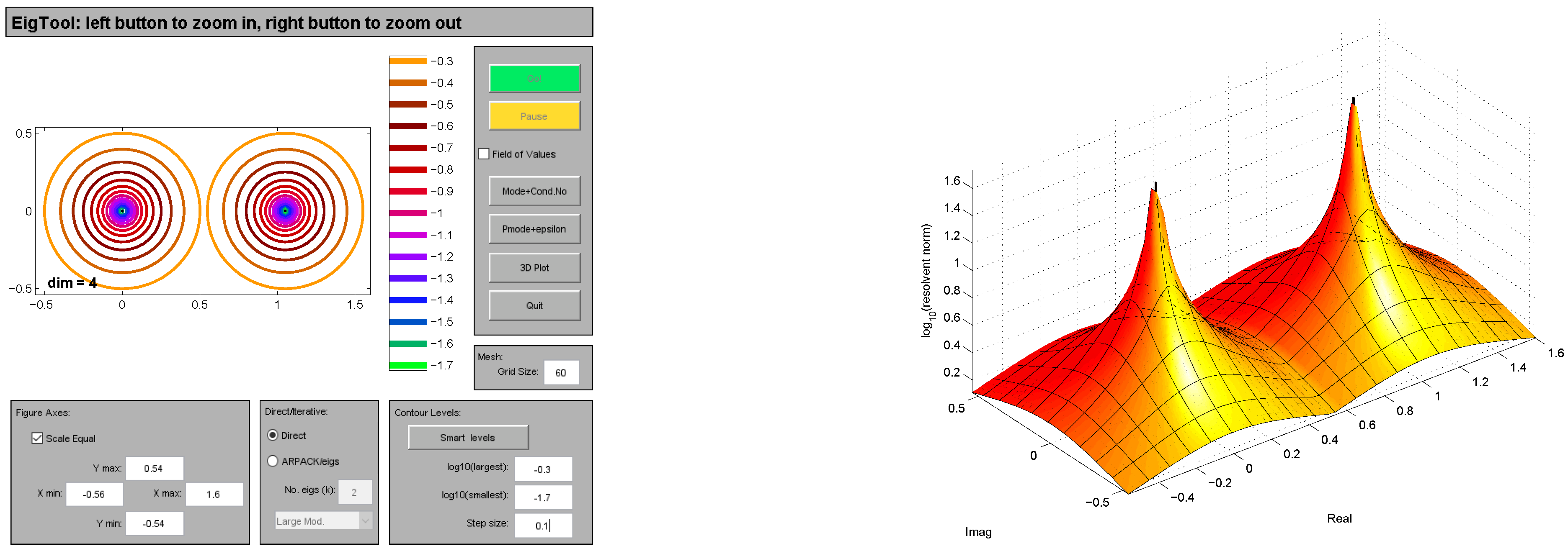
6. Numerical Experimentation

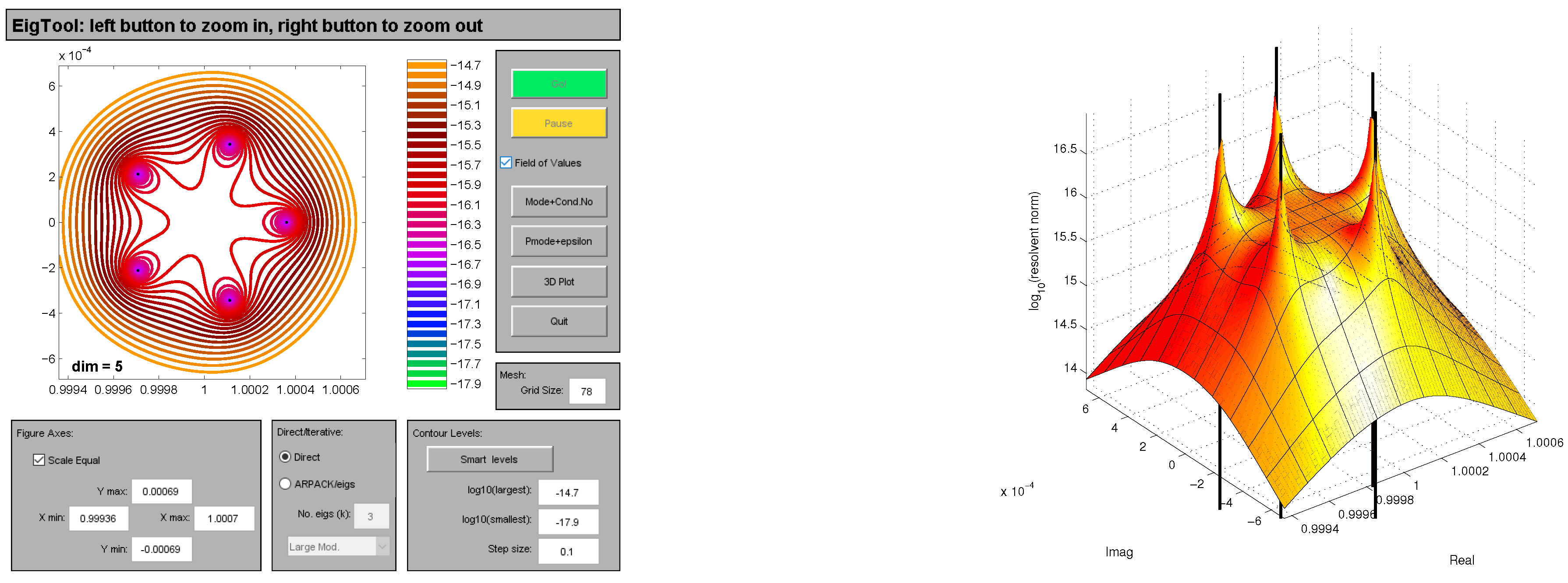
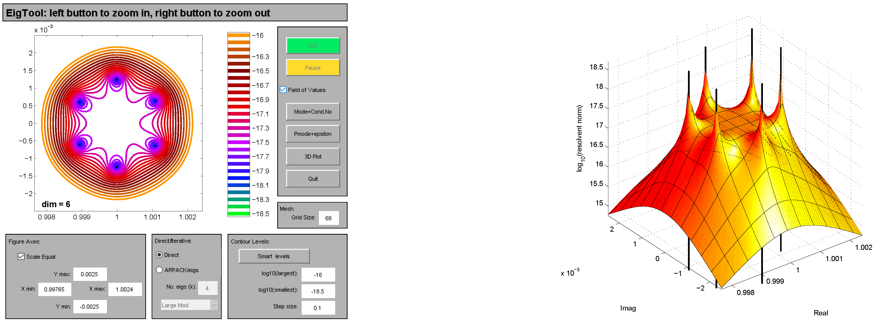
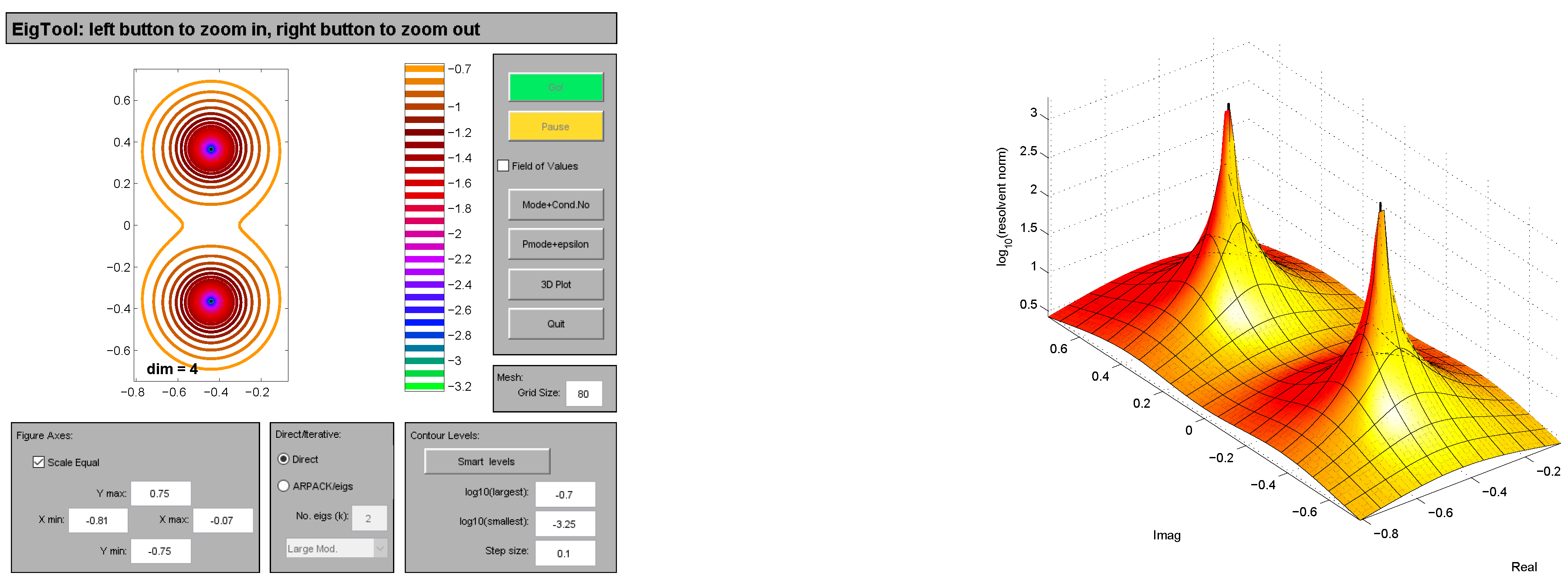
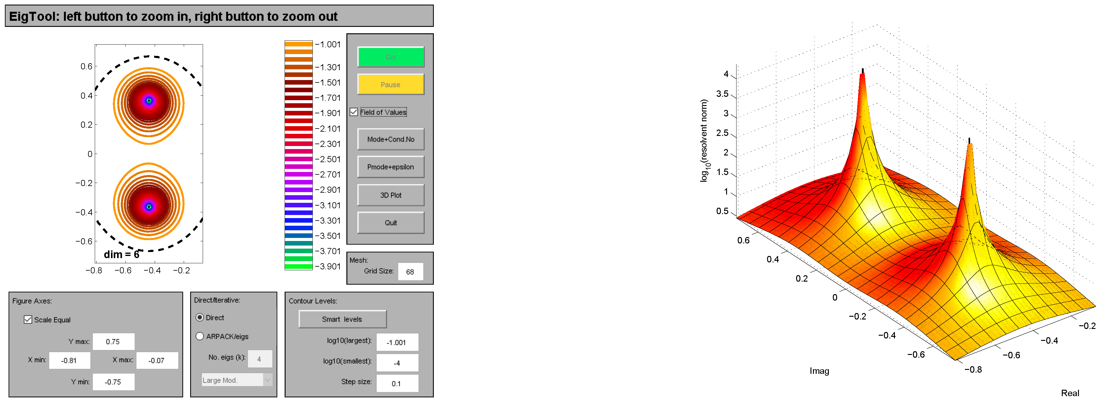
In the section we present numerical computation of the bounds of structured singular values of Toeplitz matrices [10] with various dimensions. The bounds of structured singular values are approximated with the low rank ODE’s based technique and MATLAB routine mussv. In each example, we give the comparison of bounds of structured singular values computed with low-rank ODE’s based technique and MATLAB function mussv. Furthermore, we present the pseudo-spectrum of Toeplitz matrices [10]. The software package EigTool [11] is routinely used for plotting the unstructured pseudo-spectra. In Figure 1, Figure 2, Figure 3, Figure 4, Figure 5 and Figure 6, we show the pseudo-spectrum of a variety of matrices as taken in examples 1–6. The spectrum in 3-dimensional space is also shown by making use of Eigtool.

Example 1.

Consider the real valued matrix [10].

$$M=\left[\begin{array}{ccccc}1& 0& 0& 0& 0\\ -0.5& 1& 0& 0& 0\\ 0.25& -0.5& 1& 0& 0\\ -0.125& 0.25& -0.5& 1& 0\\ 0.0625& -0.125& 0.25& -0.5& 1\end{array}\right].$$

We choose the perturbation set $\mathbb{B}=\{diag\left({\delta }_i{I}_1\right):{\delta }_i\in \mathbb{R},\forall i=1:5\}$.

Using the MATLAB function mussv, we compute an admissible perturbation $VDelta$ as

$$VDelta=1.0e+050\ast \left[\begin{array}{ccccc}5& 0& 0& 0& 0\\ 0& 5& 0& 0& 0\\ 0& 0& 5& 0& 0\\ 0& 0& 0& 5& 0\\ 0& 0& 0& 0& 5\end{array}\right].$$

The 2-norm of perturbation $VDelta$ is $5e+050$. The approximated lower and upper bounds appears 0 and $1.0005$, respectively.

Algorithm [8] computes the admissible perturbation E as

$$E=\left[\begin{array}{ccccc}1& 0& 0& 0& 0\\ 0& -1& 0& 0& 0\\ 0& 0& -1& 0& 0\\ 0& 0& 0& -1& 0\\ 0& 0& 0& 0& -1\end{array}\right].$$

The matrix 2-norm of E is computed as 1. The lower bound of structured singular value is 1, which is much tighter than the one approximated by mussv.

Example 2.

Consider the real valued matrix [10].

$$M=\left[\begin{array}{cccccc}1& 0& 0& 0& 0& 0\\ -1& 1& 0& 0& 0& 0\\ 0.5& -1& 1& 0& 0& 0\\ 0& 0.5& -1& 1& 0& 0\\ 0& 0& 0.5& -1& 1& 0\\ 0& 0& 0& 0.5& -1& 1\end{array}\right].$$

We choose the perturbation set $\mathbb{B}=\{diag\left({\delta }_i{I}_2\right):{\delta }_i\in \mathbb{R},\forall i=1:3\}$.

Using the MATLAB function mussv, we compute an admissible perturbation $VDelta$ as

$$VDelta=1.0e+050\ast \left[\begin{array}{cccccc}4.9921& 0& 0& 0& 0& 0\\ 0& 4.9921& 0& 0& 0& 0\\ 0& 0& 4.9921& 0& 0& 0\\ 0& 0& 0& 4.9921& 0& 0\\ 0& 0& 0& 0& 4.9921& 0\\ 0& 0& 0& 0& 0& 4.9921\end{array}\right].$$

Furthermore, $\parallel VDelta\parallel =4.9921e+050$. The approximated lower and upper bounds appears 0 and $1.0012$, respectively.

Using Algorithm [8], we compute the admissible perturbation E as

$$E=\left[\begin{array}{cccccc}1& 0& 0& 0& 0& 0\\ 0& 1& 0& 0& 0& 0\\ 0& 0& -1& 0& 0& 0\\ 0& 0& 0& -1& 0& 0\\ 0& 0& 0& 0& -1& 0\\ 0& 0& 0& 0& 0& -1\end{array}\right].$$

$\parallel E\parallel =1$. The lower bound of structured singular value is 1, which is much tighter than the one approximated by mussv.

Example 3.

Consider $6\times 6$ real valued matrix [10].

$$M=\left[\begin{array}{cccccc}1& 0& 0& 0& 0& 0\\ -0.6667& 1& 0& 0& 0& 0\\ 0.2500& -0.6136& 1& 0& 0& 0\\ 0& 0.2045& -0.6115& 1& 0& 0\\ 0& 0& 0.2003& -0.6096& 1& 0\\ 0& 0& 0& 0.1995& -0.6089& 1\end{array}\right],$$

and take perturbation set $\mathbb{B}=\{diag({\delta }_1{I}_3,{\delta }_2{I}_2,{\delta }_3{I}_1):{\delta }_1,{\delta }_2,{\delta }_3\in \mathbb{R}\}$.

The MATLAB functionmussvcomputes an admissible perturbation $VDelta$ as

$$VDelta=1.0e+050\ast \left[\begin{array}{cccccc}4.7266& 0& 0& 0& 0& 0\\ 0& 4.7266& 0& 0& 0& 0\\ 0& 0& 4.7266& 0& 0& 0\\ 0& 0& 0& 4.7266& 0& 0\\ 0& 0& 0& 0& 4.7266& 0\\ 0& 0& 0& 0& 0& 4.7266\end{array}\right],$$

furthermore, $\parallel VDelta\parallel =4.7266e+050$. The approximated lower and upper bounds of structured singular values are 0 and $1.0382$, respectively.

Algorithm [8] computes the admissible perturbation E with

$$E=\left[\begin{array}{cccccc}1& 0& 0& 0& 0& 0\\ 0& 1& 0& 0& 0& 0\\ 0& 0& 1& 0& 0& 0\\ 0& 0& 0& -1& 0& 0\\ 0& 0& 0& 0& -1& 0\\ 0& 0& 0& 0& 0& -1\end{array}\right],$$

having a unit matrix 2-norm. The lower bound of structured singular value is 1, which is much tighter than the one approximated by mussv.

Example 4.

Consider $4\times 4$ real valued matrix [12].

$$M=\left[\begin{array}{cccc}-0.5500& 0& -0.3300& 0\\ 0.2200& -0.5500& -0.1100& -0.3300\\ 0.4400& 0& -0.3300& 0\\ -0.7700& 0.4400& -0.2200& -0.3300\end{array}\right],$$

and we choose $\mathbb{B}=\{diag({\Delta }_1,{\Delta }_2):{\Delta }_1,{\Delta }_2\in {\mathbb{C}}^{2,2}\}$.

Using the MATLAB functionmussv, we compute an admissible perturbation $VDelta$

$$VDelta=\left[\begin{array}{cccc}-1.0009& 0.1199& 0& 0\\ 0.2860& -0.0342& 0& 0\\ 0& 0& 0.0039& -1.0140\\ 0& 0& 0.0010& -0.2662\end{array}\right].$$

where its matrix 2-norm equals $1.0483$. The lower and upper bounds of structured singular values have the same value which is $0.9539$.

Algorithm [8] computes perturbation matrix E with

$$E=\left[\begin{array}{cccc}-0.9628+0.0059i& 0.0815+0.0125i& 0& 0\\ 0.2560-0.0094i& -0.0218-0.0027i& 0& 0\\ 0& 0& 0.0062+0.0056i& -0.9558-0.0088i\\ 0& 0& 0.0019+0.0018i& -0.2935-0.0103i\end{array}\right],$$

where the unit matrix is 2-norm. The lower bound of structured singular value is $0.9537$.

Example 5.

Consider $6\times 6$ real valued matrix [12].

$$M=\left[\begin{array}{cccccc}-0.5500& 0& 0& -0.3300& 0& 0\\ 0.2200& -0.5500& 0& -0.1100& -0.3300& 0\\ 0& 0.2200& -0.5500& 0& -0.1100& -0.3300\\ 0.4400& 0& 0& -0.3300& 0& 0\\ -0.7700& 0.4400& 0& -0.2200& -0.3300& 0\\ 0& -0.7700& 0.4400& 0& -0.2200& -0.3300\end{array}\right],$$

and we choose the perturbation set $\mathbb{B}=\{diag({\Delta }_1,{\Delta }_2):{\Delta }_1,{\Delta }_2\in {\mathbb{C}}^{3,3}\}$.

Using the MATLAB functionmussv, we compute an admissible perturbation $VDelta$ as

$$VDelta=\left[\begin{array}{cccccc}-0.0773& 0.4197& -0.0400& 0& 0& 0\\ 0.1599& -0.8679& 0.0827& 0& 0& 0\\ -0.0379& 0.2058& -0.0196& 0& 0& 0\\ 0& 0& 0& -0.0292& 0.0364& -0.1338\\ 0& 0& 0& -0.1996& 0.2490& -0.9152\\ 0& 0& 0& -0.0479& 0.0598& -0.2197\end{array}\right].$$

The largest singular value of perturbation $VDelta$ is $1.0068$. The lower and upper bounds of structured singular values is the same, that is, $0.9933$.

Algorithm [8] computes the admissible perturbation E as

$$E=\left[\begin{array}{cccccc}0& 0& -0.7540+0.6569i& 0& 0& 0\\ 0& 0& 0& 0& 0& 0\\ 0& 0& 0& 0& 0& 0\\ 0& 0& 0& 0& 0& -0.9914+0.1306i\\ 0& 0& 0& 0& 0& 0\\ 0& 0& 0& 0& 0& 0\end{array}\right],$$

with $\parallel E\parallel =1$ while the lower bound of structured singular values is $0.2858$.

Example 6.

Consider $3\times 3$ real valued symmetric Toeplitz matrix.

$$M=\left[\begin{array}{ccc}1& 2& 3\\ 2& 1& 2\\ 3& 2& 1\end{array}\right].$$

We take the perturbation set $\mathbb{B}=\{diag({\delta }_1{I}_1,{\delta }_2{I}_1,{\delta }_3{I}_1):{\delta }_1,{\delta }_3\in \mathbb{C},{\delta }_2\in \mathbb{R}\}$.

Using the MATLAB functionmussv, we compute an admissible perturbation $VDelta$ with

$$VDelta=\left[\begin{array}{ccc}0.1754& 0& 0\\ 0& 0.1754& 0\\ 0& 0& 0.1754\end{array}\right].$$

The largest singular value of perturbation matrix $VDelta$ is $0.1754$. The lower and upper bounds of structured singular values are same, that is, $5.7016$.

Algorithm [8] computes the admissible perturbation E with

$$E=\left[\begin{array}{ccc}1& 0& 0\\ 0& 1& 0\\ 0& 0& 1\end{array}\right],$$

and a unit matrix 2-norm while lower bound of structured singular value is same as computed with MATLAB routine mussv, that is, $0.1754$.

7. Conclusions

The numerical computation of lower bounds of structured singular values for a family of Toeplitz matrices arising in linear time invariant feedback control systems is presented. Our results provide a characterization of gradient system of ordinary differential equations. The numerical experimentation show that in most cases our results for the computation of lower bounds of structured singular values are much tighter than the one approximated by classical methods presented in the literature and implemented in MATLAB. Using the MATLAB function mussv, we approximate the lower and upper bounds of structured singular values.