Very Long Baseline Interferometry Observations of the Proposed Radio Counterpart of an EGRET Source

Abstract

We present high-resolution radio interferometric imaging observations of the radio source NVSS J182659+343113 (hereafter J1826+3431), the proposed radio counterpart of the $\gamma$-ray source, 3EG J1824+3441 detected by the Energetic Gamma Ray Experiment Telescope (EGRET) on board the Compton Gamma Ray Observatory satellite. We analyzed eight epochs of archival multi-frequency very long baseline interferometry data. We imaged the asymmetric core–jet structure of the source, and detected apparent superluminal motion in the jet. At the highest observing frequency, $15.3$ GHz, the core shows high brightness temperature indicating Doppler boosting. Additionally, the radio features undergo substantial flux density variability. These findings strengthen the previous claim of the association of the blazar J1826+3431 with the possible $\gamma$-ray source, 3EG J1824+3441.

1. Introduction

Blazars are radio-loud active galactic nuclei (AGN) seen at a very small angle to the jet direction. The relativistic speed of the emitting plasma in the jet and the small angle to the line of sight give rise to various relativistic effects such as apparent superluminal motion and relativistic Doppler boosting of the radiation. Due to the latter, the emission of the approaching jet is enhanced while that of the receding jet (also called counterjet) is diminished significantly. The jet-to-counterjet flux density ratio can be as high as 1000 [1]. As a consequence, only the approaching one of the originally symmetrically launched jets can be observed, thus blazars appear asymmetric in that regard. The jet emission is explained as synchrotron radiation from electrons and/or positrons moving with relativistic speeds in magnetic fields. The jet synchrotron radiation is responsible for the lower-energy bump seen in the broad-band spectral energy distribution (SED) of blazars, peaking between millimetre-wavelength and X-ray regimes [2].

Blazars constitute the most populous group of extragalactic $\gamma$-ray emitter sources according to the observations of the Fermi Large Area Telescope (LAT; e.g., [3]). The $\gamma$-ray emission, responsible for the higher-energy bump in the blazar SEDs, is usually attributed to inverse-Compton process in leptonic models (e.g., [2] and references therein) or to synchrotron radiation from heavy charged particles, e.g., protons ([4] and references therein) in hadronic models. The seed photons of the inverse-Compton radiation can originate from within or external to the jet. In the former case, they are the low-energy synchrotron photons in the jet (i.e., synchrotron self-Compton process [5]), or in the latter case, the seed photons can come from the accretion disk, the broad line region, from the dusty torus or from the cosmic microwave background radiation.

Prior to Fermi, the EGRET instrument on board the Compton Gamma Ray Observatory (CGRO) satellite created the first all-sky $\gamma$-ray map above 100 MeV. The third EGRET catalogue (3EG, [6]) contains 271 sources, 94 of them showed possible or probable associations with blazars [7]. Follow-up studies (e.g., [8] and references therein) significantly increased the number of identified northern hemisphere EGRET sources at high Galactic latitudes ($\left|b\right|>{10}^{\circ }$). More than half of the 116 northern EGRET sources, 66, are found to have plausible blazar-like counterparts [8].

One of them, 3EG J1824+3441, is associated with a flat-spectrum radio quasar at a redshift $z=1.81$. This radio source was detected in the NRAO VLA Sky Survey (NVSS, [9]). J1826+3431 has a 1.4-GHz flux density of $(470\pm 14)$ mJy which is the highest value in the EGRET positional error box (∼$1^{\circ }$) [10]. Since the source belongs to the Very Long Baseline Array (VLBA) Calibrator Survey [11] sample, high-resolution radio interferometric observations of the source exist, which can be used to strengthen or falsify its inferred blazar nature and in turn its association with the EGRET $\gamma$-ray source. The accurate radio position (http://hpiers.obspm.fr/icrs-pc/newwww/icrf/icrf3sx.txt) of J1826+3431 in the current 3rd realization of the International Celestial Reference Frame [12] is right ascension ${18}^{\mathrm{h}}{26}^{\min }59.9828210\pm {0.0000091}^{\mathrm{s}}$ and declination 34${}^{\circ }$31${}^{\prime }$ 14.119974 ± 0.0019${}^{\prime \prime }$.

Throughout this paper, we assume a flat $\Lambda$CDM cosmological model with $H_0=70\mathrm{km}{\mathrm{s}}^{-1}{\mathrm{Mpc}}^{-1}$, ${\mathsf{\Omega }}_{\Lambda }=0.73$, and ${\mathsf{\Omega }}_{\mathrm{m}}=0.27$. In this model, the luminosity distance of the source at $z=1.81$ is 14 103.7 Mpc, and 1 milli-arcsecond (mas) angular size corresponds to 8.66 pc projected linear size [13].

2. Archival Radio Data

2.1. VLBI Data

In the very long baseline interferometry (VLBI) image database of the astrogeo.org website (http://astrogeo.org/ maintained by L. Petrov), there are four epochs of dual-band $2.3$- and $8.3/8.7$-GHz observations and three epochs of $15.3$ GHz measurements available of J1826+3431 between 1996 and 2018. In each of these observations, all ten antennas of the VLBA participated. Further details of the observations are given in Table 1.

Table 1. Summary of archival VLBI observations of J1826+3431. Asterisk (*) denotes the observation conducted by the EVN. All other observations were done by the VLBA.

Epoch	Project ID	Frequency	Bandwidth	On-Source Integration Time
		(GHz)	(MHz)	(min)
$1996.370$	BB023	$2.3$	32	$50.3$
$1996.370$	BB023	$8.3$	32	$50.3$
$2003.655$	BU026	$15.3$	16	$325.3$
$2004.616$	BU026	$15.3$	16	$325.3$
$2005.427$	BU026	$15.3$	16	$328.1$
$2014.145$	EF025 *	$1.7$	128	$15.0$
$2015.064$	BG219	$2.3$	128	$1.8$
$2015.064$	BG219	$8.7$	320	$1.8$
$2017.227$	UF001	$2.3$	96	$2.2$
$2017.227$	UF001	$8.7$	384	$2.2$
$2018.437$	UG002	$2.3$	96	$2.6$
$2018.437$	UG002	$8.7$	384	$2.6$

Additionally, the source was observed with the European VLBI Network (EVN) at $1.7$ GHz on 21 February 2014 (project code: EF025, PI: S. Frey). This observation was conducted in phase-referencing mode [14], and J1826+3431 was used as the phase-reference calibrator source for one of the faint targets in that project [15]. Eight antennas of the EVN participated in the measurements: Effelsberg in Germany, the Jodrell Bank Lovell Telescope in the United Kingdom, Medicina and Noto in Italy, Onsala in Sweden, Toruń in Poland, the Westerbork Synthesis Radio Telescope in the Netherlands, and Sheshan in China. Further details of the observation are given in Table 1 and in [15].

2.2. VLA Data

The public data archive (https://archive.nrao.edu/) of the U.S. National Radio Astronomy Observatory (NRAO) lists various data sets which contain VLA observations of J1826+3431. To obtain supplementary information on the arcsec-scale extended radio structure, as well as the possible variability of the source, we selected two data sets obtained at 4.86 GHz for analysis. The experiment AS291 (PI: W.C. Saslaw) was observed at the epoch 1987.493 in the most extended A configuration of the array that provides the highest angular resolution, in our case, ∼0.5 arcsec. The second experiment from 2009.388 (project code: CALSUR) used the less extended VLA B configuration, providing resolution of a few arcsecs. The integration times spent on J1826+3431 were 219 s and 43 s in 1987 and 2009, respectively. Both experiments used 100 MHz bandwidth.

3. Data Analysis

3.1. VLBA Data

Calibrated visibility files were downloaded from the astrogeo.org website, and their hybrid mapping procedure was performed using the Caltech Difmap [16] software package. Asterisks (*) denote those epochs in Table A1, Table A2, Table A3, Table A4 where we time-averaged the calibrated data into 10-s blocks. In a process of hybrid mapping, the clean algorithm [17] was used and phase-only self-calibration was done. At the end of the procedure, steps of amplitude and phase self-calibration were performed, gradually for shorter and shorter solution time intervals down to a few minutes. Images (Figure 1) were created using natural weighting, with the visibility errors raised to the power $-1$.

Figure 1. Naturally-weighted VLBI images of J1826+3431 taken at (a) $1.7$ GHz; (b) $2.3$ GHz; (c) $8.7$ GHz; and (d) $15.3$ GHz. In each image, the elliptical Gaussian restoring beam (FWHM) is shown in the lower left corner. The positions of the circular Gaussian model components describing the brightness distributions, observational epochs, and frequencies are indicated in each image. Further details of the images are given in Table 2.

Table 2. Details of the contour maps shown in Figure 1. The restoring beam major axis position angle (PA) is measured from north through east. Further positive contour levels in Figure 1 increase by a factor of 2.

		Peak	Image	Lowest	Restoring Beam
Epoch	Frequency	Brightness	Noise Level	Contour	Major Axis	Minor Axis	PA
	(GHz)	(mJy beam${}^{-1}$)	(mJy beam${}^{-1}$)	(mJy b eam${}^{-1}$)	(mas)	(mas)	(${}^{\circ }$)
$2014.145$	$1.7$	218	$0.4$	$\pm 2.0$	$16.10$	$6.75$	$8.1$
$2018.437$	$2.3$	167	$0.4$	$\pm 1.7$	$6.23$	$3.54$	$-18.3$
$2018.437$	$8.7$	113	$0.2$	$\pm 1.0$	$1.66$	$0.99$	$-15.1$
$2005.427$	$15.3$	141	$0.4$	$\pm 1.1$	$0.93$	$0.55$	$-9.6$

3.2. EVN Data

The EVN data calibration was done in the usual manner (e.g., [18]) using the NRAO Astronomical Image Processing System (AIPS, 19]). The detailed description is given in [15]. The calibrated data set was imaged in Difmap [16] using the hybrid mapping technique, which involved several steps of clean iterations interleaved by phase-only self-calibrations. When the signal-to-noise ratio in the residual image could not be improved any further, amplitude and phase self-calibration were performed. First, it was done for the whole observation; afterwards, the corrections were computed for a subset of antennas and with gradually decreasing solution time intervals down to 10 min. The image obtained is displayed in Figure 1a.

3.3. VLA Data

We performed standard amplitude and phase calibration in AIPS. The VLA flux density calibrator to set the amplitude scale was 3C 48 in both experiments. The calibrated visibility data were exported from AIPS to Difmap for hybrid mapping. The resulting clean images are shown in Figure 2.

Figure 2. Naturally-weighted 4.86-GHz VLA images of J1826+3431 taken with (a) the A configuration and (b) the B configuration of the array at the epochs 1987.493 and 2009.388, respectively. The lowest contours are (a) $\pm 0.6$ mJy beam${}^{-1}$ and (b) $\pm 1$ mJy beam${}^{-1}$. The peak brightnesses are (a) 408 mJy beam${}^{-1}$ and (b) 325 mJy beam${}^{-1}$. The restoring beams are (a) $0.{51}^{\prime \prime }\times {0.4}^{\prime \prime }$ at PA=$-{46}^{\circ }$ and (b) $6^{\prime \prime }\times 2^{\prime \prime }$ at PA=${59}^{\circ }$. In both images, the elliptical Gaussian restoring beam (FWHM) is shown at the lower left corner and the positive contours increase by a factor of 2.

3.4. Model Fitting

To describe the brightness distribution for a quantitative analysis of the source structure, we applied the technique of model fitting directly to the calibrated interferometric visibility data [20], for both the VLBI and VLA measurements. We used Difmap to represent the source brightness distribution with a set of circular Gaussian model components.

4. Results

Based on VLBI data, the inner structure of J1826+3431 shows a southeast oriented core–jet morphology consistently at all frequencies and epochs (see Figure 1 for selected example maps). The core and typically 4–5 jet features were needed to adequately model the source with circular Gaussian components at $2.3$, $8.3/8.7$, and $15.3$ GHz. At the lowest frequency, 1.7 GHz, only two model components were necessary to describe the jet brightness distribution. During the fitting procedure, all of the parameters, i.e., positions, flux densities, and full width at half-maximum (FWHM) sizes of the components were allowed to vary, except for one epoch. At $2005.427$, the fitting procedure was not able to constrain the FWHM size of the core component; therefore it was fixed at the smallest angular size resolvable with the interferometer, $0.04$ mas. To calculate this value, we used the formula given by [21]. Thus, we can only give an upper limit of the size of the core component at that epoch. The parameters of the best-fit models are summarized in Table A1, Table A2, Table A3, Table A4; the model component positions are also denoted in the images in Figure 1.

When deriving the uncertainties of the fitted parameters of the VLBI observations, we assumed $10\%$ flux density calibration uncertainties following [22]. The positional uncertainties were calculated conservatively following [23]. We quadratically added the uncertainties determined using the relations given by [24] to the $10\%$ of the restoring beam size in the cases of the core components, and to the $20\%$ of the restoring beam size when deriving the positional uncertainty of less bright jet components. To calculate the uncertainties of the FWHM sizes, we used the formula of [24].

The arcsec-scale radio structure of J1826+3431 revealed by our 4.86-GHz VLA images (Figure 2) indicates a continuing jet towards the southeast, in approximately the same position angle as the mas-scale VLBI jet (Figure 1). The jet can be traced out to ∼2.5${}^{\prime \prime }$ (corresponding to ∼20, kpc projected distance from the core) in the higher-resolution A-configuration image. There is an indication of a sharp right-angle bend towards south, as supported by the lower-resolution B-configuration VLA image where the radio emission seems extended in that direction (Figure 2). The sum of the flux densities in the fitted Gaussian model components ($428\pm 21$ mJy at 1987.493 and $333\pm 17$ mJy at 2009.388) provide evidence for significant variability.

5. Discussion

5.1. Component Proper Motions in the Mas-Scale Jet of J1826+3431

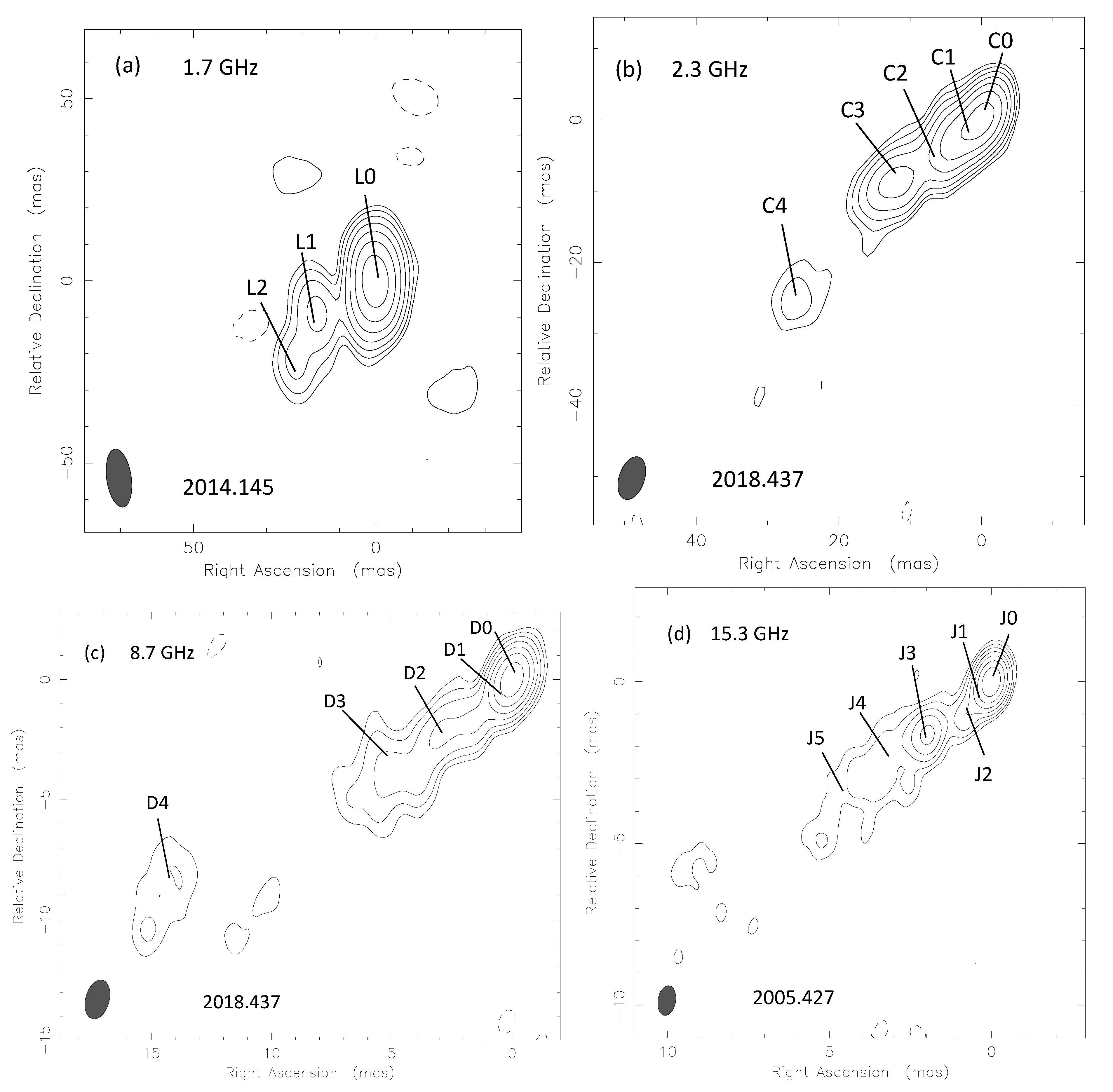
To identify the jet components throughout the full time span of the VLBI observations, we considered their positions, FWHM sizes, and flux densities. The components that are identified across the different epochs are denoted by the same identifiers in Table A2, Table A3, Table A4. The core component is numbered with 0 at each epoch and frequency; thus, it is denoted as L0, C0, D0, and J0 at $1.7$, $2.3$, $8.3/8.7$, and $15.3$ GHz, respectively.

For further analysis, we assumed the core to be stationary and we derived the positions of the fitted jet components relative to it (Table A1, Table A2, Table A3, Table A4). The jet components are assumed to move away from the core at constant speeds along a straight trajectory. Thus, we fitted their core separations with linear functions. The derived angular proper motions were converted to apparent speeds in units of the speed of light, c, using the relation [1]

$${\beta }_{\mathrm{app}}=\frac{\mu d_{\mathrm{L}}}{c(1+z)}$$

(1)

where $\mu$ is the angular proper motion of the component in rad s${}^{-1}$, $d_{\mathrm{L}}$ is the luminosity distance in m, c is the speed of light in m s${}^{-1}$, and z is the redshift of the source.

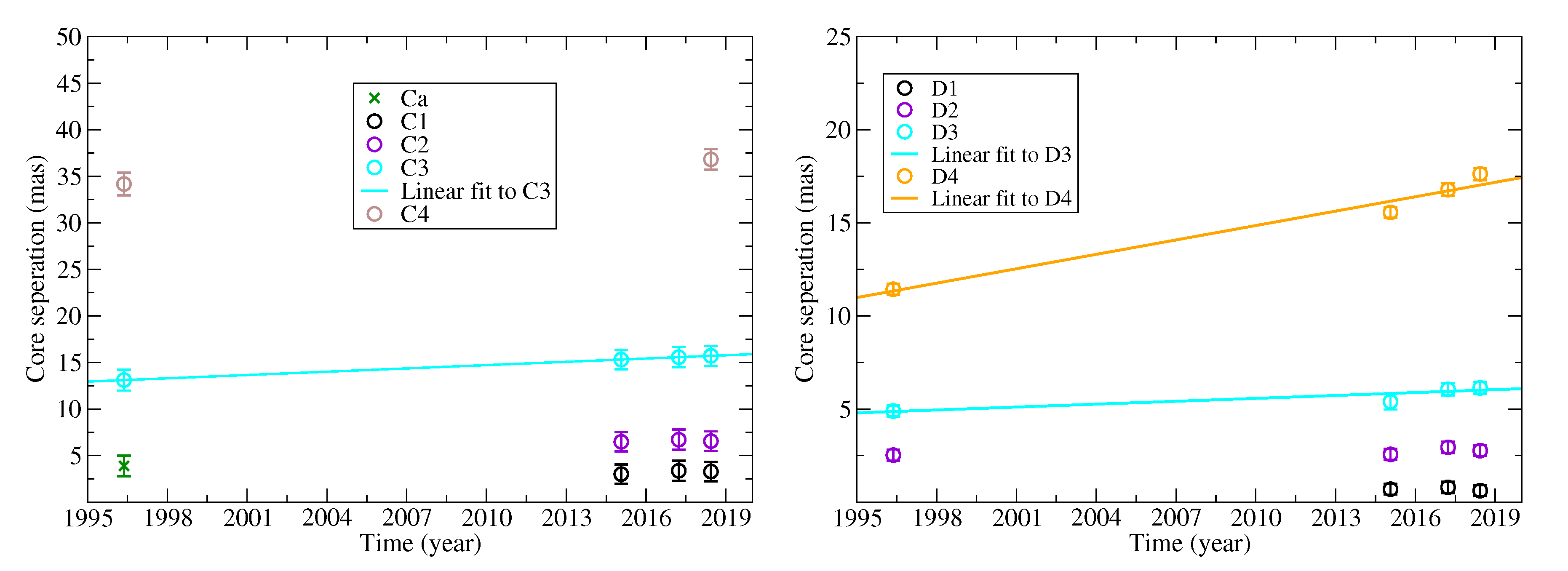
At $2.3$ GHz, at most five components were needed to describe the jet structure. The inner ≤10 mas region of the jet could not be resolved into two distinct components in $1996.370$, unlike at later epochs (components C1 and C2). Therefore, the single fitted inner jet component, Ca, cannot be unambiguously identified with either of the components detected later. Thus, the motion of C1 and C2 can only be tracked at the relatively closely-spaced observing epochs of the 2010s. Because of the short time baseline, these two components show no significant change in their core separation during the available observing epochs. On the other hand, component C3 could be unambiguously identified through all epochs. It shows an angular proper motion of $\mu =0.12\pm 0.07$ mas yr${}^{-1}$, which corresponds to an apparent speed of ${\beta }_{\mathrm{app}}=9.4\pm 5.5$. At large core separations, component C4 could only be detected at two epochs. Therefore, it is unsuitable for further proper motion calculations. The core separations for each component and the fitted linear proper motion curve for C3 are shown in Figure 3.

Figure 3. Radial separations of the components from the core as a function of time; solid lines denote the linear fit to the data. Left panel: For the observations conducted at $2.3$ GHz Right: For the observations conducted at $8.3/8.7$ GHz. The size of the error bars is roughly the same as the size of the symbols.

At $8.3/8.7$ GHz, three jet components, D2, D3, and D4, can be detected at all four epochs, while D1 can only be detected at the last three epochs. This may indicate that it was ejected some time between the epochs $1996.370$ and $2015.064$. No discernible proper motions could be detected for components D1 and D2, while D3 and D4 show apparent superluminal motions (Table 3). 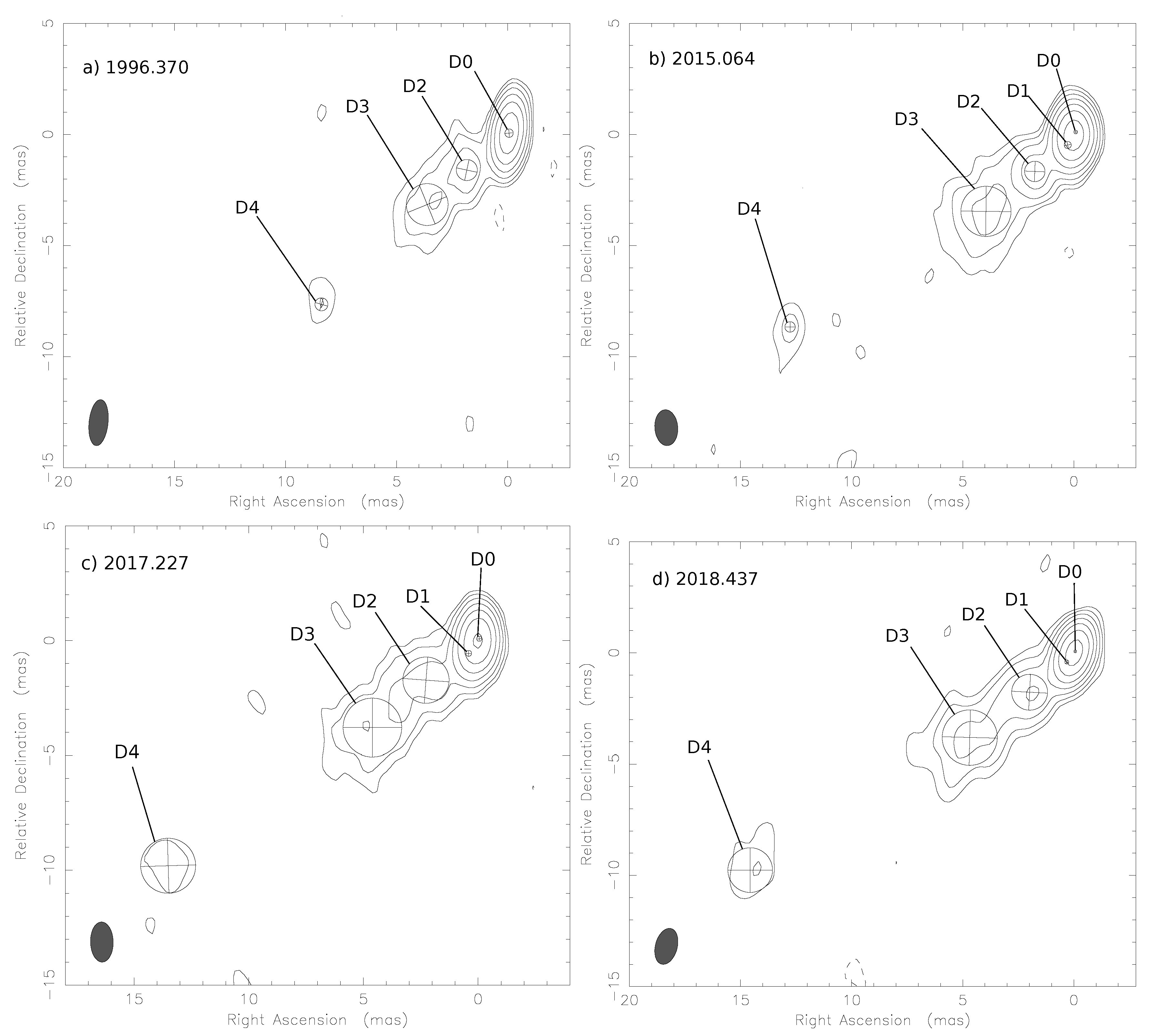The core separations and the fitted linear curves for D3 and D4 are shown in Figure 3. As we performed proper motion and jet parameter calculations using D3 and D4, we present contour maps of J1826+3431 made at this frequency at all four epochs in Figure 4, indicating the fitted model components.

Table 3. Parameters describing the movements of the components identified at $8.3/8.7$ GHz. The component identification, the angular proper motion, and the apparent jet speed in units of c are given in columns 1, 2, and 3, respectively.

ID	$\mathit{\mu }$ (mas year${}^{-1}$)	${\mathit{\beta }}_{\mathbf{app}}$
D3	$0.06\pm 0.02$	$4.8\pm 1.6$
D4	$0.28\pm 0.02$	$22.2\pm 1.6$

Figure 4. Naturally-weighted VLBI images of J1826+3431 at epochs (a) 1996.370; (b) 2015.064; (c) 2017.227; and (d) 2018.437 taken at $8.3/8.7$ GHz restored with the Gaussian model components fitted to the visibility data. The location and size (FWHM) of the model components are indicated with circles. In each image, the elliptical Gaussian restoring beam (FWHM) is shown at the lower left corner. Further details of the images are given in Table 4.

Table 4. Details of the contour maps shown in Figure 4. The restoring beam major axis position angle (PA) is measured from north through east. Further positive contour levels in Figure 4 increase by a factor of 2.

	Peak	Image	Lowest	Restoring Beam
Epoch	Brightness	Noise Level	Contour	Major Axis	Minor Axis	PA
	(mJy beam${}^{-1}$)	(mJy beam${}^{-1}$)	(mJy beam${}^{-1}$)	(mas)	(mas)	(${}^{\circ }$)
$1996.370$	$0.157$	$0.5$	$\pm 2.8$	$2.08$	$0.86$	$-6.1$
$2015.064$	$0.175$	$0.3$	$\pm 1.8$	$1.62$	$1.04$	$4.5$
$2017.227$	$0.121$	$0.3$	$\pm 1.7$	$1.75$	$0.99$	$-1.3$
$2018.437$	$0.113$	$0.2$	$\pm 1.3$	$1.66$	$0.99$	$-15.1$

At $15.3$ GHz, only three years elapsed between the first and last observations. This time span is too short for detecting proper motions in any of the fitted components. Component J1 could be first detected at epoch $2004.616$. This may indicate that J1 was ejected some time between the first and second epochs. Later, as it moved farther away from the core, this component became detectable even at a lower frequency, $8.7$ GHz, at the epoch $2015.064$ as D1.

To summarize, apparent superluminal motions could be detected in three components at relatively larger core separations (C3, D3 and D4) in the jet of J1826+3431. Interestingly, the highest apparent speed is shown by a component (D4) located at the largest core separation (∼10 mas) implying acceleration in the jet. Acceleration is often detected in the jets of blazars (e.g., [25]), and although it usually takes place at smaller core separations, there are examples for faster components further down the jets (e.g., PMN J0405−1308 [25,26], PKS 2201+171 [27]).

5.2. Relativistic Beaming in J1826+3431

At the highest observing frequency, $15.3$ GHz, which provides the best angular resolution, we derived the brightness temperature of the core component using the following equation [28]:

$$T_{\mathrm{b}}=1.22·{10}^{12}(1+z)\frac{S}{{\theta }^2{\nu }^2}\mathrm{K},$$

(2)

where S is the flux density of the fitted component in Jy, $\theta$ is the FWHM diameter of the circular Gaussian in mas, and $\nu$ is the observing frequency in GHz.

In $2003.655$, we were unable to resolve the core region into two components as at the later epochs. As a test, we tried to fit the innermost region with an elliptical Gaussian component and the resulting fit confirmed that the core was elongated in the direction of component J1 detected at the later epochs. Therefore, J0 and J1 were blended in $2003.655$, thus the FWHM size and the flux density are overestimates of the core parameters at this epoch. Since the brightness temperature is inversely proportional to the square of the FWHM size, its derived value can be regarded as a lower limit, ≥$2.8\times {10}^{11}$ K. In $2004.616$, the obtained brightness temperature is $T_{\mathrm{b}}=(12.3\pm 1.4)\times {10}^{11}$ K. At epoch $2005.427$, we could only derive an upper limit for the size of the core component, thus only a lower limit for the brightness temperature can be given, ≥12 × 10${}^{11}$ K. The lower limits agree with the $T_{\mathrm{b}}$ estimate made at the middle epoch within its errors.

All brightness temperature values exceed the equipartition limit, $T_{\mathrm{int}}\approx 5\times {10}^{10}$ K [29], indicating relativistic beaming in the source. The relativistic beaming can be quantified by the Doppler boosting factor, ${\delta }_{\mathrm{vlbi}}$, which can be estimated from the measured $T_{\mathrm{b}}$ value and the equipartition brightness temperature limit using the following relation [1]:

$${\delta }_{\mathrm{vlbi}}=\frac{T_{\mathrm{b}}}{T_{\mathrm{int}}}.$$

(3)

The obtained brightness temperature value corresponds to a Doppler factor of ${\delta }_{\mathrm{vlbi}}=24.6\pm 2.9$.

5.3. Jet Parameters

The jet parameters, the bulk Lorentz factor ($\gamma$), and the inclination angle with respect to the line of sight ($\varphi$) can be calculated from the Doppler factor and the apparent jet speed as [1]

$$\gamma =\frac{{\beta }_{\mathrm{app}}^2+{\delta }^2+1}{2\delta }$$

(4)

and

$$tan\varphi =\frac{2{\beta }_{\mathrm{app}}}{{\beta }_{\mathrm{app}}^2+{\delta }^2-1}.$$

(5)

The component close to the innermost core region with the best-defined positions and thus proper motion is D3; therefore, we used the apparent superluminal speed obtained for this jet feature, ${\beta }_{\mathrm{app}}^{\mathrm{D}}3=4.8\pm 1.6$, to derive the jet parameters. Using the Doppler factor obtained from the $15.3$-GHz measurement at epoch $2004.616$, we get a Lorentz factor of $\gamma =12.8\pm 1.4$, implying relativistic bulk jet velocity in units of the speed of light, $\beta =0.997\pm 0.002$. The corresponding jet inclination angle is $\varphi ={0.9}^{\circ }\pm {0.3}^{\circ }$.

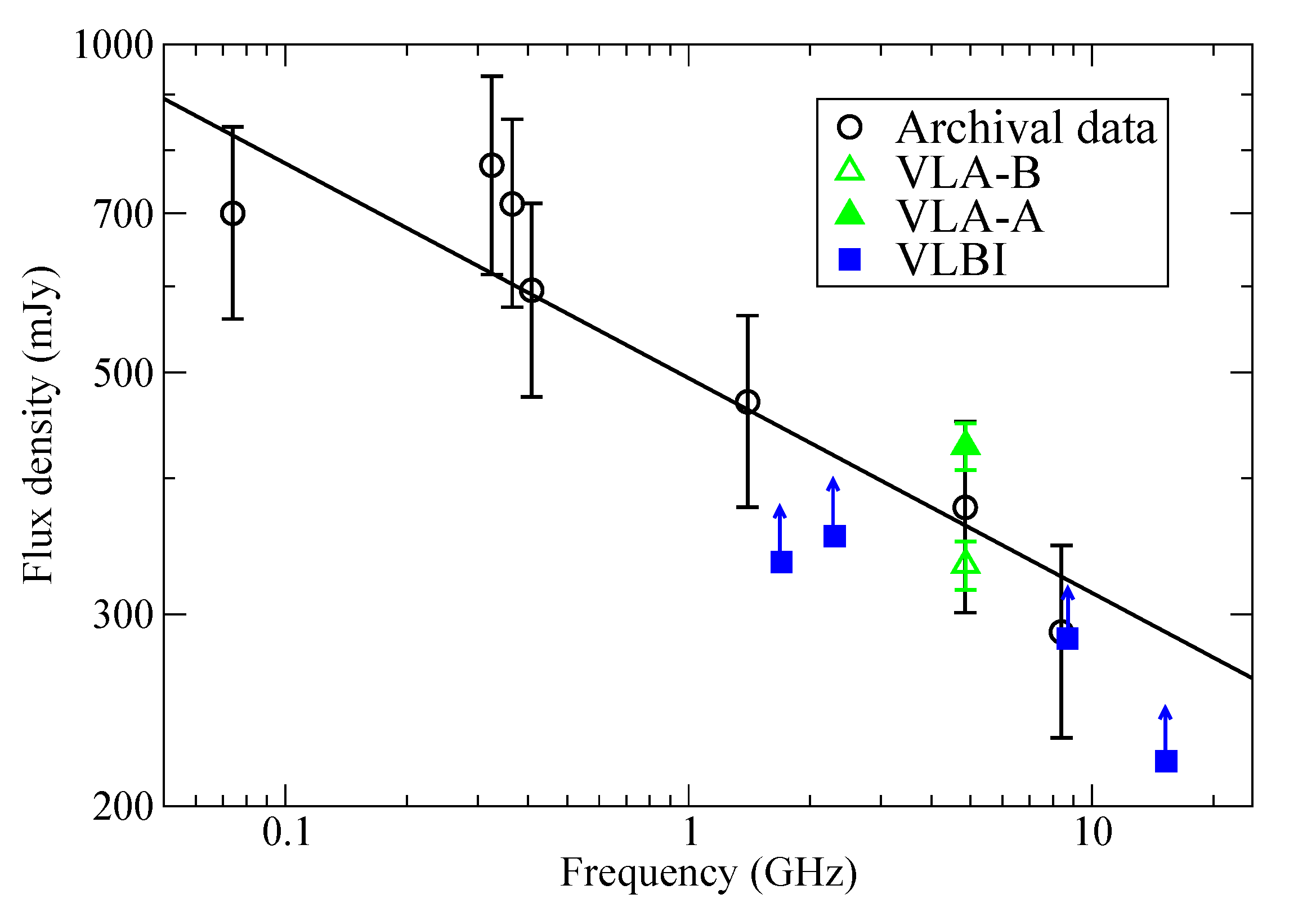
5.4. Radio Spectrum of J1826+3431

We collected the radio flux density measurements of J1826+3431 from the literature (Table 5). We fitted a power–law curve to these data points to obtain the spectral index ($\alpha$; defined as $S\propto {\nu }^{\alpha }$, where S is the flux density and $\nu$ is the observing frequency). Since the flux density measurements are not simultaneous, source variability may affect the spectral index calculation, so the value can be considered as tentative. The resulting fit is shown with a black line in Figure 5, the obtained spectral index is $\alpha =-0.19\pm 0.05$, indicating a flat spectrum.

Table 5. Archival radio flux density measurements of J1826 + 3431.

Observer Instrument	Frequency	Flux Density	Flux Density Error	Reference
	(GHz)	(Jy)	(Jy)
VLA-B, VLA-BnA	0.074	0.700	0.140	VLSS [30]
Westerbork Synthesis Radio Telescope	0.325	0.775	0.160	WN [31]
Texas Interferometer	0.365	0.714	0.140	TXS [32]
Bologna Northern Cross Telescope	0.408	0.595	0.120	B2.3 [33]
VLA-D, VLA-DnC	1.4	0.470	0.094	NVSS [9]
Green Bank 91-m telescope	4.85	0.376	0.075	87GB [34]
VLA-A	8.4	0.289	0.058	CLASS [35]

Figure 5. Radio spectrum of J1826+3431. Black circles are from archival measurements, their details are given in Table 5. Green triangles indicate the sum of modelfit components of the VLA measurements presented in this paper. Black line represents the power-law fit to the above total flux density points. Blue squares with arrows show the sum of modelfit components of high-resolution VLBI measurements from this paper, as lower limits to the total flux density. The selected VLBA epochs ($2015.064$ for $2.3$ and $8.7$ GHz, and $2005.427$ for $15.3$ GHz) are the closest in time to the $1.7$-GHz EVN measurement.

For comparison, we also show the sum of the VLBI Gaussian model component flux densities with blue squares and upward arrows in Figure 5. For each observing frequency, we have chosen the observation that is the closest to the $1.7$-GHz EVN measurement. VLBI observations are insensitive to the large (arcsec) scale radio structure; therefore, in the presence of such emission, they underestimate the total flux density of a source. This can be seen in Figure 5 where all VLBI points are indeed below the fitted spectrum.

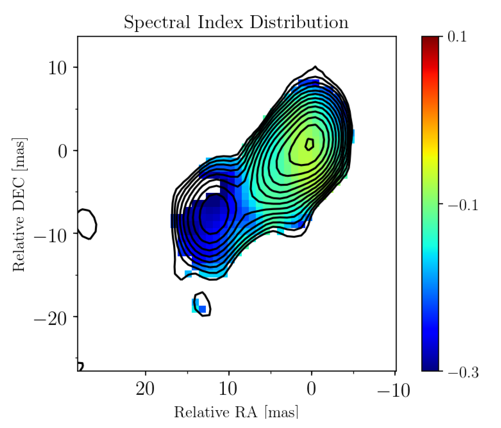
The simultaneous $2.3$- and $8.3/8.7$-GHz observations allow us to map the spectral index distribution of the mas-scale radio emission in J1826+3431 using VIMAP [36]. We present a spectral index image in Figure 6. We used our data from the epoch 2015.064. After using elliptical masks to exclude the cores from the images, we matched the $2.3$- and $8.7$-GHz maps of J1826+3431 by using two-dimensional correlation. Considering that the frequencies are relatively close to each other and that the measurements were performed at the same time, it was not necessary to shift the brightness peak. The spectral index image (Figure 6) suggests a flat-spectrum radio emission ($\alpha \approx -0.1\pm 0.1$) in the core region and along the jet closer to the core. It is in good agreement with the spectral index calculated using the archival total flux density data (Figure 5) since the dominant emission feature of the source is the core. The spectrum gradually steepens further away from the core along the jet, as expected from optically thin synchrotron radio emission.

Figure 6. Spectral index map of J1826+3431 using $2.3$- and $8.7$-GHz data taken at 2015.064. The colour bar shows the spectral index values. The contours represent the 2.3-GHz image, the lowest contour level is drawn at $3\sigma$ image noise level corresponding to 2.4 mJy beam${}^{-1}$. Further contours increase by a factor of 2. The peak intensity is 162 mJy beam${}^{-1}$. The restoring beam size is $3.69\mathrm{mas}\times 5.72\mathrm{mas}$ at $\mathrm{PA}=-{3.7}^{\circ }$.

5.5. Flux Density Variability

To characterize variability in the VLBI-detected features, we plot the sum of flux densities in the fitted Gaussian model components at different observing frequencies as a function of time in Figure 7. As can be clearly seen, especially for the 2.3- and 8.3/8.7-GHz data where the observations span more than two decades, the flux density of the source is strongly variable over time. Moreover, the variations in the difference of the 2.3- and 8.3/8.7-GHz flux density values suggest variability of the spectral index.

Figure 7. Flux density of J1826+3431 versus time at $2.3$, $8.3/8.7$, and 15.3 GHz, based on the sum of fitted VLBI model component flux densities.

5.6. $\gamma$-Ray Properties of 3EG J1824+3441

3EG J1824+3441 was detected with a weak $\gamma$-ray flux of $(28.7\pm 9.3)\times {10}^{-8}$ photon s${}^{-2}$ cm${}^{-1}$ by EGRET [6]. However, an alternate version of the EGRET catalogue [37] (see also [7]) which used reprocessed data assuming a different model for the Galactic interstellar emission does not contain as many as 107 sources previously detected in [6], including also 3EG J1824+3441. In that sense, it is not surprising that no $\gamma$-ray source is listed in the most recent fourth Fermi/LAT catalogue [3] within a $1^{\circ }$ radius of the position of the putative EGRET $\gamma$-ray source.

Alternatively, even if the source exists, long-term variability of its $\gamma$-ray flux can also explain the Fermi non-detection. Indeed, a comparison of high-confidence (>4$\sigma$) EGRET detections with the third Fermi/LAT catalogue revealed 10 extragalactic $\gamma$-ray sources missing from the latter [38]. 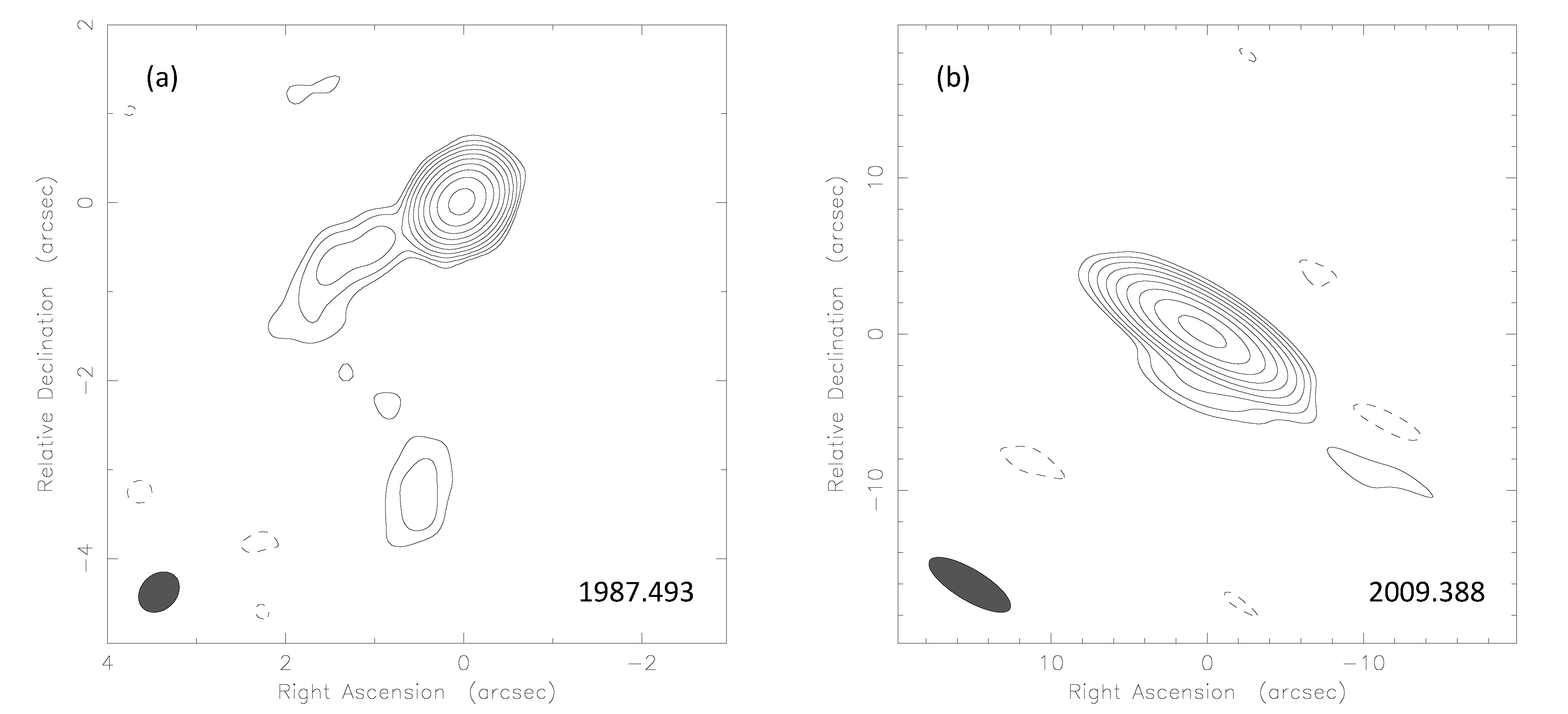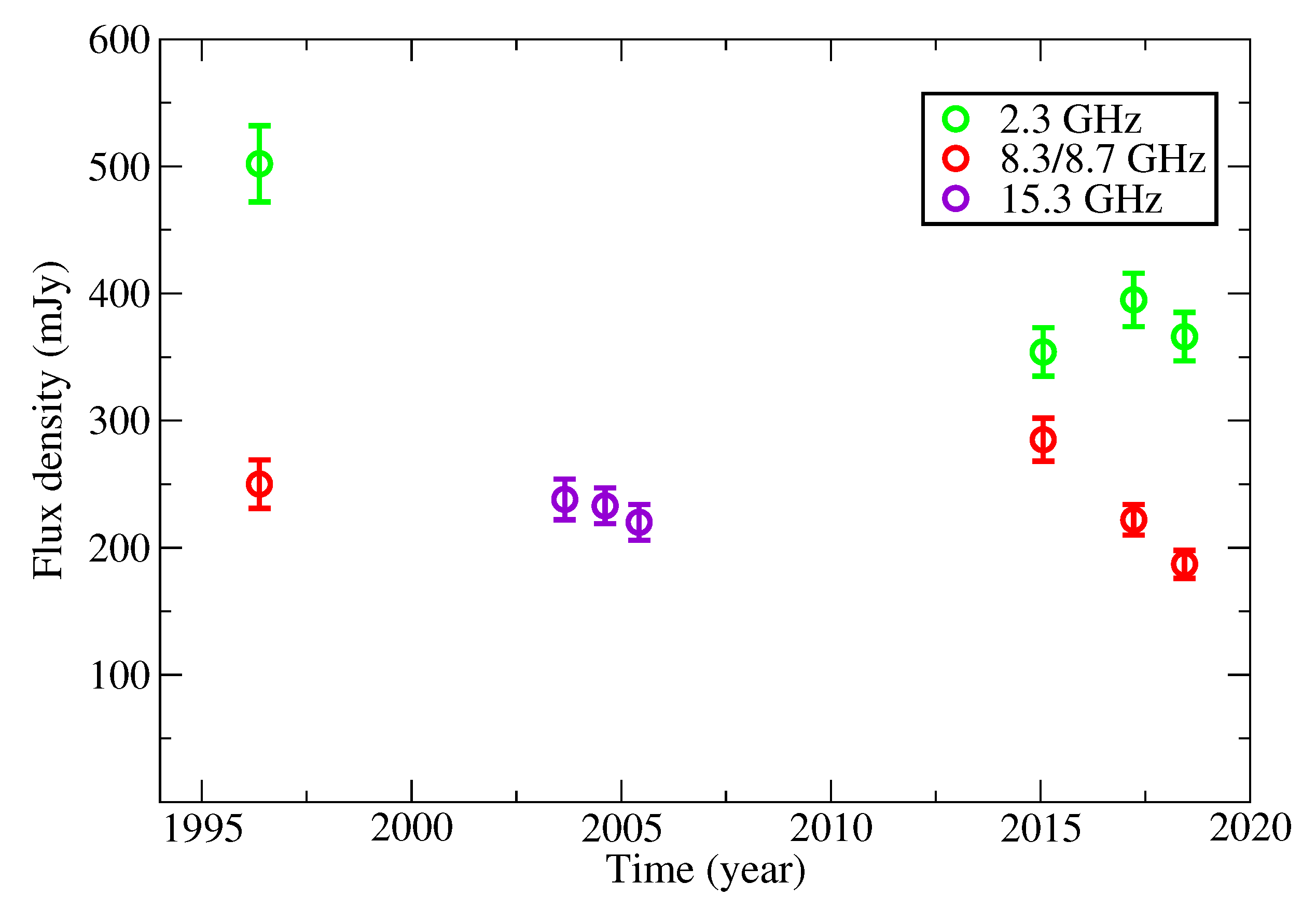Subsequent analysis of seven years of Fermi data showed that five sources were in a low-luminosity state during the Fermi observations compared to their luminosity during the EGRET observations [38]. The generally decreasing long-term trend we see in the radio flux density of the possible counterpart, the blazar J1826+3431, with respect to the 1990s when CGRO was operational (see e.g., our VLA results and Figure 7) is also consistent with a $\gamma$-ray flux decrease.

6. Conclusions

We analyzed eight epochs of high-resolution multi-frequency VLBI data of the radio source J1826+3431, which is the proposed radio counterpart of the EGRET $\gamma$-ray source, 3EG J1824+3441. The archival observations span a period of more than 22 years. Each data set was imaged, and the brightness distribution of the source was modeled using circular Gaussian components, in order to characterize the physical and geometric properties of the jet and to analyze the kinematics of J1826+3431. One and two moving jet components could be securely identified at multiple epochs in the $2.3$- and $8.3/8.7$-GHz data, respectively. All of them showed outward motion with apparent superluminal speed. The estimated brightness temperature of the most compact component, the core at $15.3$ GHz suggests that the radio emission is relativistically beamed in the source. From the relativistic effects seen in the radio jet and the strong variability of the core component at the measured frequencies, the radio source J1826+3431 can be identified as a blazar. Since the vast majority of extragalactic $\gamma$-ray sources are associated with blazars, we can conclude that J1826+3431 is very likely the radio counterpart of the unidentified EGRET source 3EG J1824+3441. However, no $\gamma$-ray source is found at this position in the latest Fermi/LAT catalogue [3], and its detection can be regarded uncertain based on an alternative version of the EGRET catalogue [37].

References

- Urry, C.M.; Padovani, P. Unified Schemes for Radio-Loud Active Galactic Nuclei. Publ. Astron. Soc. Pac. 1995, 107, 803. [Google Scholar] [CrossRef]
- Giommi, P.; Padovani, P.; Polenta, G.; Turriziani, S.; D’Elia, V.; Piranomonte, S. A simplified view of blazars: Clearing the fog around long-standing selection effects. Mon. Not. R. Astron. Soc. 2012, 420, 2899–2911. [Google Scholar] [CrossRef]
- Abdollahi, S.; Acero, F.; Ackermann, M.; Ajello, M.; Atwood, W.B.; Axelsson, M.; Baldini, L.; Ballet, J.; Barbiellini, G.; Bastieri, D.; et al. Fermi Large Area Telescope Fourth Source Catalog. Astrophys. J. Suppl. Ser. 2020, 247, 33. [Google Scholar] [CrossRef]
- Rani, B.; Krichbaum, T.P.; Hodgson, J.A.; Zensus, J.A. Location and origin of gamma-rays in blazars. J. Phys. Conf. Ser. 2016, 718, 052032. [Google Scholar] [CrossRef]
- Dermer, C.D. On the Beaming Statistics of Gamma-Ray Sources. Astrophys. J. Lett. 1995, 446, L63. [Google Scholar] [CrossRef]
- Hartman, R.C.; Bertsch, D.L.; Bloom, S.D.; Chen, A.W.; Deines-Jones, P.; Esposito, J.A.; Fichtel, C.E.; Friedlander, D.P.; Hunter, S.D.; McDonald, L.M.; et al. The Third EGRET Catalog of High-Energy Gamma-Ray Sources. Astrophys. J. Suppl. Ser. 1999, 123, 79–202. [Google Scholar] [CrossRef]
- Thompson, D.J. Gamma ray astrophysics: The EGRET results. Rep. Prog. Phys. 2008, 71, 116901. [Google Scholar] [CrossRef]
- Sowards-Emmerd, D.; Romani, R.W.; Michelson, P.F. The Gamma-Ray Blazar Content of the Northern Sky. Astrophys. J. 2003, 590, 109–122. [Google Scholar] [CrossRef][Green Version]
- Condon, J.J.; Cotton, W.D.; Greisen, E.W.; Yin, Q.F.; Perley, R.A.; Taylor, G.B.; Broderick, J.J. The NRAO VLA Sky Survey. Astron. J. 1998, 115, 1693–1716. [Google Scholar] [CrossRef]
- Bhattacharya, D.; Akyüz, A.; Miyagi, T.; Samimi, J.; Zych, A. On the distribution of EGRET unidentified sources in the Galactic plane. Astron. Astrophys. 2003, 404, 163–170. [Google Scholar] [CrossRef]
- Gordon, D.; Jacobs, C.; Beasley, A.; Peck, A.; Gaume, R.; Charlot, P.; Fey, A.; Ma, C.; Titov, O.; Boboltz, D. Second Epoch VLBA Calibrator Survey Observations: VCS-II. Astron. J. 2016, 151, 154. [Google Scholar] [CrossRef] [PubMed]
- Charlot, P.; Jacobs, C.S.; Gordon, D.; Lambert, S.; de Witt, A.; Böhm, J.; Fey, A.L.; Heinkelmann, R.; Skurikhina, E.; Titov, O.; et al. The third realization of the International Celestial Reference Frame by very long baseline interferometry. Astron. Astrophys. 2020. [Google Scholar] [CrossRef]
- Wright, E.L. A Cosmology Calculator for the World Wide Web. Publ. Astron. Soc. Pac. 2006, 118, 1711–1715. [Google Scholar] [CrossRef]
- Beasley, A.J.; Conway, J.E. VLBI Phase-Referencing. In Very Long Baseline Interferometry and the VLBA; Zensus, J.A., Diamond, P.J., Napier, P.J., Eds.; Astronomical Society of the Pacific Conference Series; Astronomical Society of the Pacific: San Francisco, CA, USA, 1995; Volume 82, p. 327. [Google Scholar]
- Frey, S.; Paragi, Z.; Gabányi, K.É.; An, T. Four hot DOGs in the microwave. Mon. Not. R. Astron. Soc. 2016, 455, 2058–2065. [Google Scholar] [CrossRef]
- Shepherd, M.C.; Pearson, T.J.; Taylor, G.B. DIFMAP: An interactive program for synthesis imaging. Bull. Astron. Soc. 1994, 26, 987–989. [Google Scholar]
- Högbom, J.A. Aperture Synthesis with a Non-Regular Distribution of Interferometer Baselines. Astron. Astrophys. Suppl. 1974, 15, 417–426. [Google Scholar]
- Diamond, P.J. VLBI Data Reduction in Practice. In Very Long Baseline Interferometry and the VLBA; Zensus, J.A., Diamond, P.J., Napier, P.J., Eds.; Astronomical Society of the Pacific Conference Series; Astronomical Society of the Pacific: San Francisco, CA, USA, 1995; Volume 82, p. 227. [Google Scholar]
- Greisen, E.W. AIPS, the VLA, and the VLBA. In Information Handling in Astronomy—Historical Vistas; Heck, A., Ed.; Astrophysics and Space Science Library; Springer: Dordrecht, The Netherlands, 2003; Volume 285, p. 109. [Google Scholar] [CrossRef]
- Pearson, T.J. Non-Imaging Data Analysis. In Very Long Baseline Interferometry and the VLBA; Zensus, J.A., Diamond, P.J., Napier, P.J., Eds.; Astronomical Society of the Pacific Conference Series; Astronomical Society of the Pacific: San Francisco, CA, USA, 1995; Volume 82, p. 267. [Google Scholar]
- Kovalev, Y.Y.; Kellermann, K.I.; Lister, M.L.; Homan, D.C.; Vermeulen, R.C.; Cohen, M.H.; Ros, E.; Kadler, M.; Lobanov, A.P.; Zensus, J.A.; et al. Sub-Milliarcsecond Imaging of Quasars and Active Galactic Nuclei. IV. Fine-Scale Structure. Astron. J. 2005, 130, 2473–2505. [Google Scholar] [CrossRef]
- Karamanavis, V.; Fuhrmann, L.; Krichbaum, T.P.; Angelakis, E.; Hodgson, J.; Nestoras, I.; Myserlis, I.; Zensus, J.A.; Sievers, A.; Ciprini, S. PKS 1502+106: A high-redshift Fermi blazar at extreme angular resolution. Structural dynamics with VLBI imaging up to 86 GHz. Astron. Astrophys. 2016, 586, A60. [Google Scholar] [CrossRef]
- Lister, M.L.; Cohen, M.H.; Homan, D.C.; Kadler, M.; Kellermann, K.I.; Kovalev, Y.Y.; Ros, E.; Savolainen, T.; Zensus, J.A. MOJAVE: Monitoring of Jets in Active Galactic Nuclei with VLBA Experiments. VI. Kinematics Analysis of a Complete Sample of Blazar Jets. Astron. J. 2009, 138, 1874–1892. [Google Scholar] [CrossRef]
- Fomalont, E.B. Image Analysis. In Synthesis Imaging in Radio Astronomy II; Taylor, G.B., Carilli, C.L., Perley, R.A., Eds.; Astronomical Society of the Pacific Conference Series; Astronomical Society of the Pacific: San Francisco, CA, USA, 1999; Volume 180, p. 301. [Google Scholar]
- Lister, M.L.; Aller, M.F.; Aller, H.D.; Homan, D.C.; Kellermann, K.I.; Kovalev, Y.Y.; Pushkarev, A.B.; Richards, J.L.; Ros, E.; Savolainen, T. MOJAVE: XIII. Parsec-scale AGN Jet Kinematics Analysis Based on 19 years of VLBA Observations at 15 GHz. Astron. J. 2016, 152, 12. [Google Scholar] [CrossRef]
- Hervet, O.; Boisson, C.; Sol, H. An innovative blazar classification based on radio jet kinematics. Astron. Astrophys. 2016, 592, A22. [Google Scholar] [CrossRef]
- Lister, M.L.; Homan, D.C.; Hovatta, T.; Kellermann, K.I.; Kiehlmann, S.; Kovalev, Y.Y.; Max-Moerbeck, W.; Pushkarev, A.B.; Readhead, A.C.S.; Ros, E.; et al. MOJAVE. XVII. Jet Kinematics and Parent Population Properties of Relativistically Beamed Radio-loud Blazars. Astrophys. J. 2019, 874, 43. [Google Scholar] [CrossRef]
- Condon, J.J.; Condon, M.A.; Gisler, G.; Puschell, J.J. Strong radio sources in bright spiral galaxies. II. Rapid star formation and galaxy-galaxy interactions. Astrophys. J. 1982, 252, 102–124. [Google Scholar] [CrossRef]
- Readhead, A.C.S. Equipartition Brightness Temperature and the Inverse Compton Catastrophe. Astrophys. J. 1994, 426, 51. [Google Scholar] [CrossRef]
- Cohen, A.S.; Lane, W.M.; Cotton, W.D.; Kassim, N.E.; Lazio, T.J.W.; Perley, R.A.; Condon, J.J.; Erickson, W.C. The VLA Low-Frequency Sky Survey. Astron. J. 2007, 134, 1245–1262. [Google Scholar] [CrossRef]
- Rengelink, R.B.; Tang, Y.; de Bruyn, A.G.; Miley, G.K.; Bremer, M.N.; Roettgering, H.J.A.; Bremer, M.A.R. The Westerbork Northern Sky Survey (WENSS), I. A 570 square degree Mini-Survey around the North Ecliptic Pole. Astron. Astrophys. Suppl. 1997, 124, 259–280. [Google Scholar] [CrossRef]
- Douglas, J.N.; Bash, F.N.; Bozyan, F.A.; Torrence, G.W.; Wolfe, C. The Texas Survey of Radio Sources Covering −35.5 degrees < declination < 71.5 degrees at 365 MHz. Astron. J. 1996, 111, 1945. [Google Scholar] [CrossRef]
- Colla, G.; Fanti, C.; Fanti, R.; Ficarra, A.; Formiggini, L.; Gandolfi, E.; Gioia, I.; Lari, C.; Marano, B.; Padrielli, L.; et al. The B2 catalogue of radio sources - third part. Astron. Astrophys. Suppl. 1973, 11, 291. [Google Scholar]
- Gregory, P.C.; Condon, J.J. The 87GB Catalog of Radio Sources Covering 0 degrees < delta < +75 degrees at 4.85 GHz. Astrophys. J. Suppl. Ser. 1991, 75, 1011. [Google Scholar] [CrossRef]
- Myers, S.T.; Jackson, N.J.; Browne, I.W.A.; de Bruyn, A.G.; Pearson, T.J.; Readhead, A.C.S.; Wilkinson, P.N.; Biggs, A.D.; Blandford, R.D.; Fassnacht, C.D.; et al. The Cosmic Lens All-Sky Survey - I. Source selection and observations. Mon. Not. R. Astron. Soc. 2003, 341, 1–12. [Google Scholar] [CrossRef]
- Kim, J.Y.; Trippe, S. VIMAP: An Interactive Program Providing Radio Spectral Index Maps of Active Galactic Nuclei. J. Korean Astron. Soc. 2014, 47, 195–199. [Google Scholar] [CrossRef]
- Casandjian, J.M.; Grenier, I.A. A revised catalogue of EGRET γ-ray sources. Astron. Astrophys. 2008, 489, 849–883. [Google Scholar] [CrossRef]
- Bhattacharya, D.; Mohana A, K.; Gulati, S.; Bhattacharyya, S.; Bhatt, N.; Sreekumar, P.; Stalin, C.S. Unusual long-term low-activity states of EGRET blazars in the Fermi era. Mon. Not. R. Astron. Soc. 2017, 471, 5008–5017. [Google Scholar] [CrossRef]
© 2020 by the authors. Licensee MDPI, Basel, Switzerland. This article is an open access article distributed under the terms and conditions of the Creative Commons Attribution (CC BY) license (http://creativecommons.org/licenses/by/4.0/).