The Application of a Hybrid Model Using Mathematical Optimization and Intelligent Algorithms for Improving the Talc Pellet Manufacturing Process

Abstract

Moisture is one of the most important factors impacting the talc pellet process. In this study, a hybrid model (HM) based on the combination of intelligent algorithms, self-organizing map (SOM), the adaptive neuron fuzzy inference system (ANFIS) and metaheuristic optimizations, genetic algorithm (GA) and particle swarm optimization (PSO) is introduced, namely, HM-GA and HM-PSO. The main purpose is to predict the moisture in the talc pellet process related to symmetry in the aspect of real-world application problem. In the combination process, SOM classifies the suitable input data. The GA and PSO, as the training algorithms of ANFIS, are investigated to compare the prediction skill. Five factors, including talc powder, water, temperature, feed speed, and air flow of 52 experiment cases designed by central composite design (CCD), are the training set data. Three different measures evaluate the capacity of moisture prediction. The comparison results show that the HM-PSO can provide the smallest difference between train and test datasets under the condition of the moisture being less than 5%. As a result, the HM-PSO model achieves the best result in predicting the moisture for the talc pellet process with R = 0.9539, RMSE = 1.0693, and AAD = 0.393, compared to others.

1. Introduction

Talc is a mineral occurring naturally in the form of crystalline hydrated magnesium silicate, with a chemical formula of M_g3SiO₁₀(OH)₂. Talc has low abrasion, high thermal conductivity and stability, low electrical conductivity, and high oil and grease adsorption [1]. Due to its unique surface chemistry, lamellar crystal habit, and properties, talc minerals are widely applied commercially and industrial, such as in cosmetics, pharmaceuticals, paints, polymers, and ceramics. Furthermore, the method evaluated the suitable properties of talc, which can contribute to the industry in terms of the efficiency of production planning.

In the talc forming process, many factors, especially moisture, plays an important role. The more accurate the moisture forecasting, the better the quality of the talc pellet. Over the last decade, artificial neural networks (ANNs) have become a popular technique for data prediction due to their high accuracy. Loveday et al. [2] apply an ANN to decrease the time for palm oil production. The developed model provides a reliable result and high efficiency. Adaptive neuro-fuzzy inference systems (ANFIS) is a kind of ANN usually applied in various fields to study, for example, economic order quality, water level prediction, medicine, and markets [3]. The ANFIS is an algorithm that combines the advantages of both ANN and fuzzy inference systems (FIS). It has the ability to capture the nonlinear structure of a process and has a rapid learning capacity [4]. In manufacturing applications, Caydas et al. [5] developed ANFIS for the prediction of a wire electrical discharge machine. Zhange and Lei [6] established ANFIS to predict the roughness of laser cutting and improve the quality level of laser cutting. Sen et al. [7] utilized ANFIS for predicting machining performance parameters of Inconel 690. The result of all research shows that the ANFIS performs with high accuracy with respect to prediction.

In recent years, a hybridization of ANFIS with many optimization algorithms has been introduced to improve the forecasting accuracy of the traditional ANFIS. Abdollahi [8] introduced a novel hybrid model for forecasting the Australian option price market. In a hybrid process, it consists of an entropy method and ANFIS trained by PSO. Bui et al. [9] presented three new hybrid ANFIS with cultural, bee, and invasive weed optimization, namely, ANFIS-CA, ANFIS-BA, and ANFIS-IWO for flood susceptibility mapping (FSM). Yaseen et al. [10] proposed a new hybrid ANFIS with the firefly algorithm for monthly streamflow forecasting. Gocken and Boru [11] integrate the ANFIS with GA and harmony search (HS) in weather forecasting. However, GA and PSO are commonly combined with ANFIS. Oliverira and Schirru [12] apply PSO for tuning ANFIS in sensor monitoring compared to ANFIS using one gradient descendent (GD) and GA. It found that the PSO applied in ANFIS gives the best result. Alarifi et al. [13] combine PSO and GA with ANFIS to improve the prediction performance of the thermophysical properties of Al₂O₃-MWCNT/oil. Based on the result, they found that both of the ANFIS-PSO and ANFIS-GA models are able to predict the thermophysical properties appropriately. Kumar and Hynes [14] predicted and optimized the surface roughness in thermal drilling by integrating ANFIS and GA. Rezakazemi et al. [15] employed ANFIS with GA and PSO for the evaluation of H₂-selective mixed matrix membranes (MMMs). The results showed that the ANFIS with PSO is more reliable than the ANFIS with GA and the traditional ANFIS. Sabeti and Deevband [16] introduced a novel training method of ANFIS by combining PSO and GA to solve the nonlinear dynamical system. The proposed PSOGA method provides the satisfactory results.

On the other hand, the appropriate collection of input data has a fundamental impact on the performance of the ANFIS model. It may lead to a better explanation of the results. There are only a few studies that apply the method in selecting the proper input data to ANFIS. Dariane and Azimi [17] investigated appropriate input data selection in streamflow using GA and wavelet methods to deal with ANFIS applications. The results show that the performance of the model is improved when GA and wavelets are applied. Jeong et al. [18] used a wrapper method to select the suitable input variables applied to a neuro-fuzzy model in monthly precipitation forecasting. The uncertainty in forecasting can be reduced effectively. The self-organizing map (SOM), first introduced in 1990 by Kohonen [19], is an unsupervised learning method in ANN successfully established in data classification, pattern recognition, data compression, and data mining. It can reduce high-dimensional data to low-dimensional data. In manufacturing applications, SOM has been widely used for data clustering [20,21]. Some studies apply SOM to cluster the input data for ANFIS. Nourani et al. [22] identified the input data for ANFIS by SOM and the wavelet transform groundwater level (GWL) and to fill the missing GWL data. The obtained results show that the proposed model can predict reliable accuracy. Amiryousefi et al. [23] categorized the dataset into two clusters by SOM before feeding into an ANFIS model to predict the mass transfer kinetics in deep-fat frying (DFF). Nasir and Cool [24] classified the input dataset by the SOM approach and combined it with an ANN or ANFIS. The results show that the proposed model makes a powerful intelligent model for wood machining monitoring.

The moisture in Uttaradit, Thailand is estimated by local traditional drying. It cannot determine the moisture of the talc mineral before the production process. The moisture is measured step-by-step depending on the user experience and it takes a long time to obtain the information. As mentioned previously, the novel techniques based on the combination of ANFIS with GA and PSO, using the SOM-clustering method introduced to improve the forecasting accuracy in the talc pellet forming process. The related theories are briefly described in Section 2. The schematic and the procedures of the proposed model are indicated in Section 3. The result description is therefore investigated and discussed in Section 4. Finally, the overview of this study is concluded in Section 5.

2. Materials and Methods

A talc pellet is represented as material for this study. The talc pellet forming process is explained. The traditional methods, including SOM, ANFIS, GA, and PSO, are described.

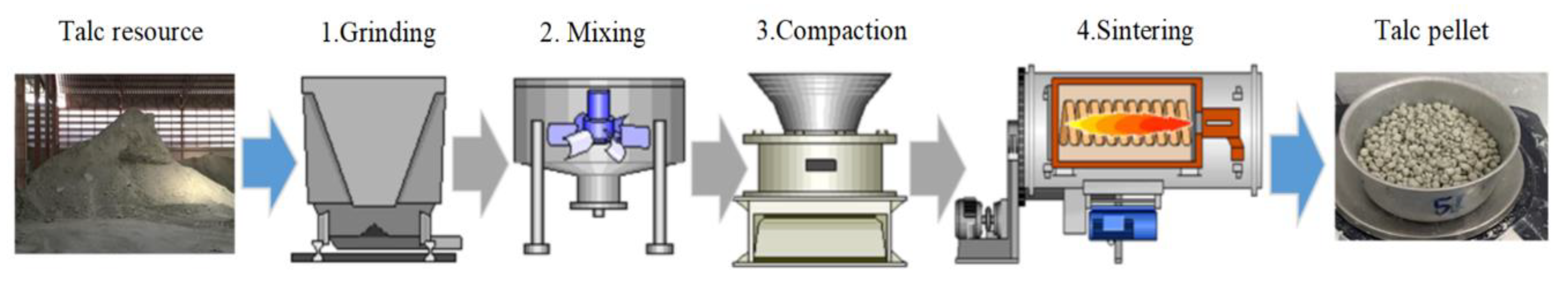
2.1. Talc Pellet Forming Process

The material used in this study is a naturally occurring mineral. It can be found in Tha Pla district, Uttaradit province, Thailand. The talc pellet forming process applies the powder metallurgy production. It includes the important process of powder production, grinding, blending, compaction, and sintering, as shown in Figure 1.

From Figure 1, the talc pellet forming process consists of five steps. Firstly, talc is ground by a Raymond mill. Secondly, the ground talc is conveyed into a mixing tank. Thirdly, the mixed talc is compacted with mechanical force by a double roller and the mixture pressed through a 5 mm sieve to form material for sintering. Fourthly, talc is sintered with LPG by using a spiral drying conveyer. Finally, the talc pellet is produced and sent to the hopper and drying tube for further use.

In talc pellet moisture measurement, talc obtained according to the testing condition from 52 experimental designs can be measured, as in the ASTM D2216-98 standard [25]. The moisture of the processed can be calculated as:

$$M_c=\frac{W_2-W_3}{W_3-W_1}\times 100,$$

(1)

where $M_C$ is the talc pellet moisture (%), $W_1$ is the weight of an empty talc container (g), $W_2$ is the weight of talc before drying (g), and $W_3$ is the weight after drying (g).

2.2. Method

2.2.1. Self-Organizing Map

The basic concept of SOM is in the concept of a transformation a complex, high-dimensional input data into a simple low-dimensional discrete output [26]. The SOM, an unsupervised learning algorithm, comprises three essential phases: competition, cooperation, and adaptation. Before training, the initial values of the learning rate, radius of the neighborhood, the number of iterations and the number of patterns, and the SOM array size are required [27].

At the start of learning the weight vector, $w_i$, is generated by a random number and input vector, x, is a random distribution which corresponds to the column index. The set of weight vectors is formed as $w_i=[w_{ij}],\mathrm{i}=1,2,\dots ,k_x,\mathrm{j}=1,2,\dots ,k_y$ where $k_x$ is the number of row and $k_y$ is the number of columns. The three phases for calculating the SOM algorithm are shown below.

In competition, the Euclidian distance between the input vector and the neuron with the weight vector of the given neuron, $w_c$, is computed as:

$$d\left(x,w\right)=\Vert x(t)-w_c(t)\Vert$$

(2)

The neuron with the most similar weight vector to the input will search for the winner neuron, the best matching unit (BMU). BMU is calculated as:

$$BMU=argmin\Vert x(t)-w_c(t)\Vert$$

(3)

In cooperation, the collected neighborhood function is used in this study is the Gaussian function, computed as:

$$h_{ij}^c=\alpha (t)\times e^{\left(-{\Vert R_c-R_{ij}\Vert }^2/2{\left({\eta }_{ij}^c\left(t\right)\right)}^2\right)}$$

(4)

The parameter ${\eta }_{ij}^c$ represents the radius of the neighborhood between nodes $w_c$ and $w_{ij}$. Two-dimensional vectors, $R_c$ and $R_{ij}$, include $w_c$ and $w_{ij}$ [28].

In adaptation, the weight vector is adjusted after obtaining the winning neuron to increase the similarity with the input vector. The rule for updating the weight vector is given by:

$$w_i(t+1)=w_i(t)+\alpha (t)h_{ij}^c(t)(x(t)-w_i(t))$$

(5)

Here, $h_{ij}^c(t)$ is a neighborhood function and t is the order number of a current iteration. The learning rate functions, $\alpha (t)$ is defined as follows:

$$\alpha (t,T)=\alpha (0)\times e^{\frac{t}{T}}$$

(6)

Here, T is the number of total iterations and t is the order number of a current iteration [28]. However, it is under the condition ${\eta }_{ij}^c\le \left[\alpha max(k_x{k}_y),1\right]$ for all cases of analysis.

The percent of occurrence or frequency of each pattern is the number of occurrences divided by the total number of samples. The probability that specific humidity would map to any pattern is 1/n, where n is the number of patterns. The significance of the frequency can be determined by calculating the 95% confidence interval around the expected probability of 1/n. Assuming that the process is a binomial, the 95% confidence limits are calculated by:

$$p\pm 1.96{\left[\frac{p\left(1-p\right)}{N}\right]}^{1/2}$$

(7)

where p is the probability that any sample maps to any pattern and N is the number of input vector used to train the map [27].

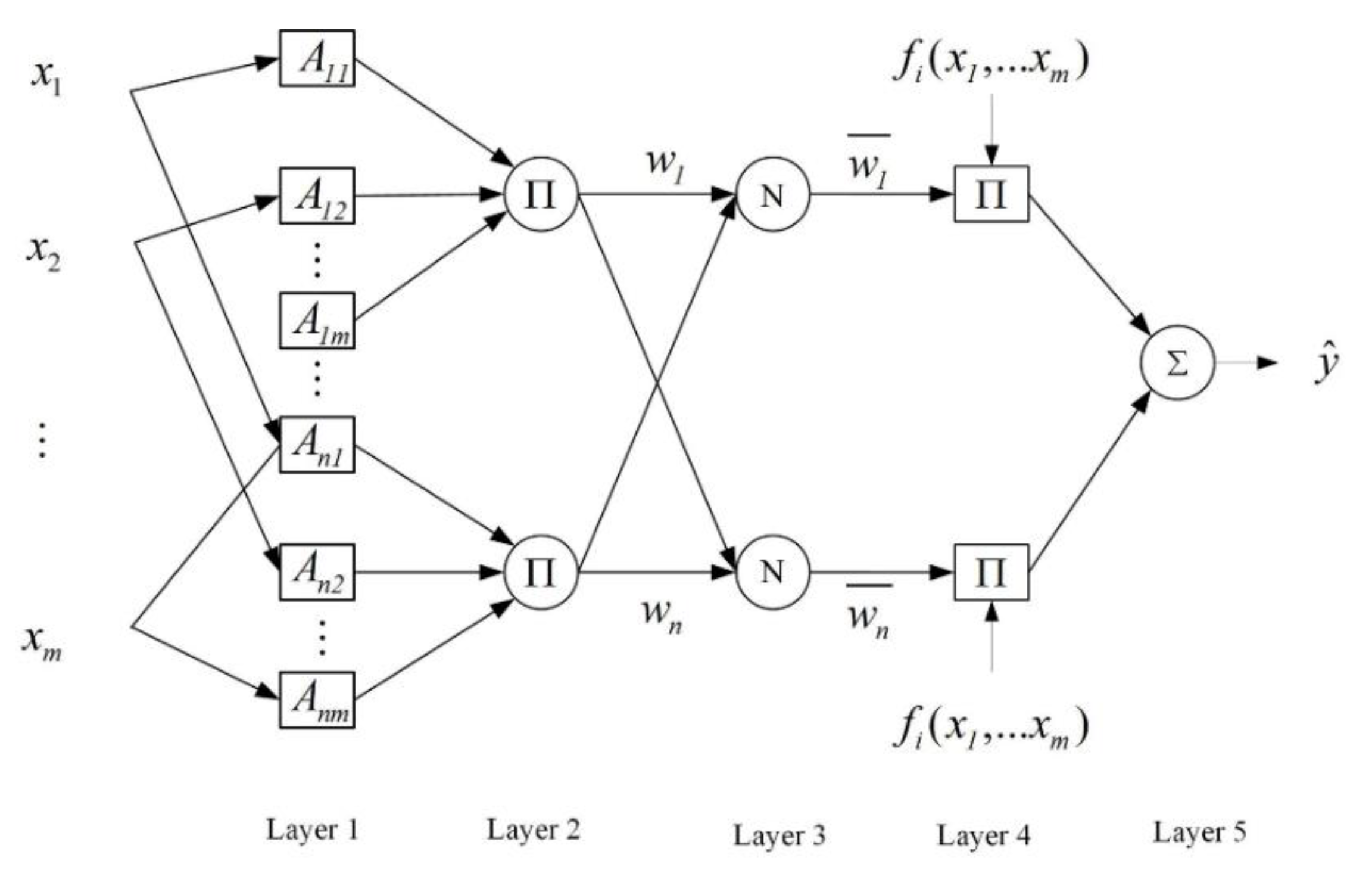
2.2.2. Adaptive Neuro-Fuzzy Inference System

The adaptive neuro-fuzzy inference system (ANFIS) was first introduced in 1993 by Jang [29]. It is the method that powerfully integrates ANNs and fuzzy inference systems (FIS). For constructing a set of fuzzy, if-then rules with appropriate membership are applied to determine the relationship between the input and output variables. There are two inference systems in fuzzy logic while the inference system of Takagi–Sugeno–Kang is usually applied [13]. Figure 2 shows the structure of ANFIS.

From Figure 2, there are five layers in ANFIS. The fuzzy if-then rules are considered to explain the rule of each layer as follows:

$$\mathrm{If}{x}_i\mathrm{is}{A}_{i1}\mathrm{AND}\dots \mathrm{AND}{x}_m\mathrm{is}{A}_{im}\mathrm{then}{y}_i\mathrm{is}{f}_1=x_1,\dots ,x_m$$

(8)

• Layer 1: Adjust every node by using Equation (9):

  $$O_i^1={\mu }_{ij}(x)$$

  (9)

From Equation (8), ${\mu }_{ij}(x)$ is a Gaussian function computed by ${\mu }_{A_{ij}}(\mathrm{x})=\exp \left(-{(x_j-c_i)}^2/2s_{ij}^2\right)$ where $c_{ij}$ is the midpoint value and $s_{ij}$ is the standard deviation value of the input variable at $x_j$.

• Layer 2: Calculate each node by multiplying the fuzzy value. The output is calculated as:

  $$O_i^2=w_i={\displaystyle \prod _{j=1}^m{A}_i{}_j}(x_i)$$

  (10)
• Layer 3: Sum the fuzzy value of every node to one value by:

  $$O_i^3={\overline{w}}_i=\frac{w_i}{{\displaystyle {\sum }_{i=1}^n{w}_i}}$$

  (11)
• Layer 4: Normalize the fuzzy value of every node by:

  $$O_i^4={\overline{w}}_i{f}_i$$

  (12)

  where $f_i$ are the consequent parameters from Takag–Sugeno–Kang’s pattern.
• Layer 5: Sum all output from layer four to obtain the final output by:

  $$O_i^5={\displaystyle \sum _{i=1}^n{\overline{w}}_i{f}_i}$$

  (13)

2.2.3. The ANFIS Training Algorithm

Genetic Algorithm

The genetic algorithm (GA) is one of the most effective algorithms in metaheuristic optimization, first presented by [30] and completed in 1989 by [31]. GA is an imitated process of natural selection and genetics to find the optimal formula for predicting. The basic procedures of GA are as follows.

• Chromosome encodes: Design the chromosomes as the system-represented solution by using any encoding method on the solving condition.
• Population initialization: Initialize the prototype population at the beginning of GA. The first population group is randomly created by matching with the defined population size.
• The fitness function: Define the score of each possible solution. Every chromosome implies the fitness of the inheritance consideration for themselves in order to create the next-generation chromosome.
• Selection: Select the genetic operator that supports the worthy member to transfer into the next generation. The process of selecting the best chromosome among the whole population is normally selected by good origin for good species according to the natural selection concept.
• Crossover: The copying of the new chromosome is pasted at a random position of the father and behind the random position of the mother to become the first offspring chromosome. The second offspring chromosome occurs by the same process as the first offspring while switching the position of the father and mother.
• Mutation: Mutate the value of the chromosome. The mutation process randomly mutates the position under the mutation possibility by changing some genes on the chromosome.
• Replacement: Replace the previous generation chromosomes with mutated chromosomes.
• Termination condition: Terminate the procedure when the condition is satisfied.

Particle Swarm Optimization

Particle swarm optimization (PSO), invented for solving the non-linear optimization introduced by Kennedy and Eberhart [32], is based on the concept of the foraging of bird flock behavior to find the optimized solution area. Each of the birds in the flock is represented with the particle. In each particle, the fitness value implies the distance between the particle and food source as having the best fitness value in each interval the fitness value of the particle which be found by the Equation (14):

$$f(x_1,x_2,x_3,\dots x_n)=f(x)$$

(14)

In defining the particle, $x_i$ is the defined fitness function. Accordingly, PSO begins with randomizing a set of particle positions, then optimizing by adjusting the parameters in each decision cycle. Each particle keeps their best position value, $P_{best,i}$ during that interval, including the whole particle best position data, in every process interval t, and the movement speed would be adjusted by using $P_{best,i}$ and $G_{best}$, which can be demonstrated by Equation (15) at the next time step, t + 1, where $t\in [0,\dots ,N]$ and can be calculated by Equation (16) at time step t, respectively [33]:

$$P_{best,i}^{t+1}=\{\begin{array}{ll}{P}_{best,i}^{t+1}& iff(x_t^{t+1})>P_{best,i}^t\\ x_i^{t+1}& iff(x_t^{t+1})\le P_{best,i}^t\end{array}$$

(15)

$$G_{best}=\min \left\{P_{best,i}^{t+1}\right\},\mathrm{where}i\in [1,\dots ,n]\mathrm{and}n>1$$

(16)

where $P_{best,i}$ is the best position that the individual particle, i has visited since the first time step, $G_{best}$ is the best position discovered by any of the particles in the entire swarm, where $P_{best,i}$ is the best particle. In this method, each individual particle, $i\in [1,\dots ,n]$, where n > 1, has been calculated in the search space $x_i$. The new velocity is calculated as in Equation (17):

$$v_{ij}^{t+1}=\omega *v_{ij}^t+c_1{r}_{1j}^t[P_{best,i}^t-x_{ij}^t]+c_2{r}_{2j}^t[G_{best}-x_{ij}^t]$$

(17)

where $v_{ij}^t$ is the velocity of the particle i in the dimension j of time t, ω is an inertia weight, $x_{ij}^t$ is a position, $P_{{}_{best,i}}^t$ is the best position of a particle, $G_{best}$ is the best position of the whole particle system, $c_1$ and $c_2$ are the constant accelerations in searching, and $r_{1j}^t$ and $r_{2j}^t$ are the random numbers between 0 and 1 at time t.

2.2.4. Performance Evaluation

In order to evaluate the superiority of the model generated by ANFIS, three techniques, absolute average deviation (AAD), root mean square error (RMSE), and correlation coefficient (R), are applied. R (Equation (18)) is used to measure how close the predicted value is to the experimental value. The closer each of these values is to 1 indicates a better prediction. RMSE (Equation (19)) and AAD (Equation (20)) are employed to investigate the accuracy of the model predictions [34]:

$$R=\frac{{\displaystyle \sum _{i=1}^N(Q_i-\overline{Q})(E_i-\overline{E})}}{\sqrt{{\displaystyle \sum _{i=1}^N{(Q_i-\overline{Q})}^2{\displaystyle \sum _{i=1}^N{(E_i-\overline{E})}^2}}}}$$

(18)

$$RMSE=\sqrt{\frac{1}{N}{\displaystyle \sum _{i=1}^N(Q_i-E}{)}^2}$$

(19)

$$AAD=\frac{1}{N}{\displaystyle \sum _{i=1}^N\left|\frac{E_i-Q_i}{Q_i}\right|}$$

(20)

where Q is the target value, E is the prediction value, and N is the total number of input data.

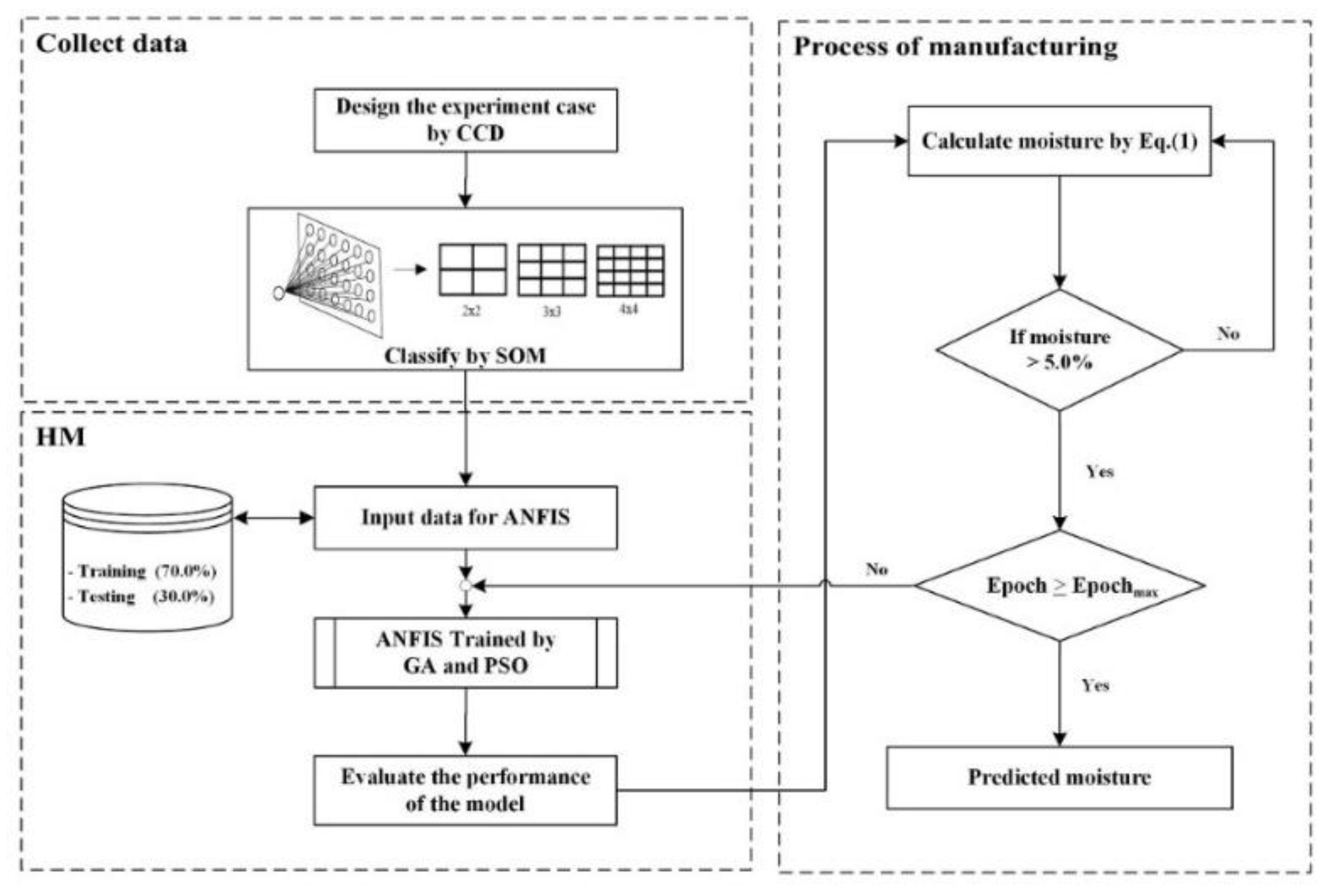
3. The Proposed Model

In this section, the proposed model is introduced. It is a novel technique based on a combination of SOM and ANFIS. The experimental design is described in Section 3.1. The hybrid model is introduced in Section 3.2, and the experiment setting is determined in Section 3.3.

3.1. The Experimental Design

In order to design the experiment, the central composite design (CCD) of the response surface methodology (RSM) is applied [35]. There are five factors influencing the talc pellet forming process in predicting the proper moisture. The input data consists of talc powder, water, temperature, feed speed, and air flow. According to the CCD, the maximum and minimum values of each variable are adjusted, as shown in

Table 1. The value of α in the talc pellet forming process.

Factor	Symbol	The Value of α					Unit
		1.682	1.0	0	−1.0	−1.682
Talc	Ta	18.6892	18	17.5	17	16.3107	kg
Water	W	4.3446	4	3.75	3.5	3.1553	kg
Temperature	Temp	191.35	150	120	90	48.65	°C
Feed Speed	FS	0.56	0.43	0.34	0.24	0.11	m/min
Air Flow	AF	8.40	7.21	6.35	5.48	4.29	m/sec

. It consists of 52 experiments cases as shown in

Table 2. The data of experimental design.

No.	Ta	W	Temp	FS	AF	MC	No.	Ta	W	Temp	FS	AF	MC
1	17	3.5	90	0.24	7.21	6.31	27	17.5	3.75	120	0.34	6.35	1.38
2	18	3.5	90	0.24	5.48	2.89	28	17.5	3.75	120	0.34	6.35	2.33
3	17	4	90	0.24	5.48	3.94	29	17.5	3.75	120	0.34	6.35	3.85
4	18	4	90	0.24	7.21	7.02	30	17.5	3.75	120	0.34	6.35	3.75
5	17	3.5	150	0.24	5.48	0.56	31	17.5	3.75	120	0.34	6.35	3.07
6	18	3.5	150	0.24	7.21	0.51	32	17.5	3.75	120	0.34	6.35	2.56
7	17	4	150	0.24	7.21	0.39	33	17	3.5	90	0.24	5.48	4.19
8	18	4	150	0.24	5.48	0.42	34	18	4	90	0.24	5.48	5.37
9	17	3.5	90	0.43	5.48	11.17	35	17	3.5	150	0.24	7.21	0.45
10	18	3.5	90	0.43	7.21	8.96	36	17	4	150	0.24	5.48	0.41
11	17	4	90	0.43	7.21	7.86	37	18	3.5	90	0.43	5.48	7.47
12	18	4	90	0.43	5.48	8.76	38	17	4	90	0.43	5.48	6.16
13	17	3.5	150	0.43	7.21	1.41	39	17	3.5	150	0.43	5.48	4.34
14	18	3.5	150	0.43	5.48	2.61	40	18	3.5	150	0.43	7.21	1.08
15	17	4	150	0.43	5.48	2.22	41	17.5	3.75	120	0.34	6.35	3
16	18	4	150	0.43	7.21	0.85	42	17.5	3.75	120	0.34	6.35	3.33
17	16.31	3.75	120	0.34	6.35	2.11	43	18	4	150	0.43	5.48	2.39
18	18.69	3.75	120	0.34	6.35	1.64	44	18	3.5	90	0.24	7.21	5.61
19	17.5	3.16	120	0.34	6.35	1.56	45	17	4	90	0.24	7.21	4.66
20	17.5	4.34	120	0.34	6.35	3.19	46	18	3.5	150	0.24	5.48	0.62
21	17.5	3.75	49	0.34	6.35	15.36	47	18	4	150	0.24	7.21	0.4
22	17.5	3.75	191	0.34	6.35	0.36	48	17	3.5	90	0.43	7.21	4.74
23	17.5	3.75	120	0.11	6.35	0.66	49	18	4	90	0.43	7.21	8.38
24	17.5	3.75	120	0.56	6.35	7.7	50	17	4	150	0.43	7.21	1.28
25	17.5	3.75	120	0.34	4.29	5.54	51	17.5	3.75	120	0.34	6.35	3.04
26	17.5	3.75	120	0.34	8.4	2.21	52	17.5	3.75	120	0.34	6.35	3.25

.

According to Table 1, by using CCD, the maximum value of five input data, the scale value for α rotatability relative to ±1.0 in this study is tested at 2.378 when implemented in the real experiment, but the forming process failed when the scaling value for finding optimal α rotatability is changed at 2.00, 1.682, and 1.414, and also with rotatability values of −2.00, −1.682, and −1.414, respectively [36]. The experimental results found that α = 1.682 can be applied to the real forming process.

3.2. A Hybrid Model

A hybrid model (HM) is introduced based on the combination between SOM and ANFIS trained by GA and PSO. There are two main processes, including SOM and ANFIS, with two training algorithms: GA and PSO. Firstly, the SOM algorithm is applied to classify the appropriate input data before feeding into the ANFIS. Secondly, the selected input data are computed by ANFIS. In ANFIS, GA and PSO are employed as training algorithms. The HM trained by GA and PSO are called HM-GA and HM-PSO, respectively. The schematic of the proposed model is shown in Figure 3.

3.3. The Experimental Setting

In order to set the appropriate parameters of SOM, ANFIS, GA, and PSO, there are no theoretical existing criteria [37].

Table 3. Parameter setting of ANFIS and SOM.

SOM	Value	ANFIS	Value
Initial learning rate	0.85	Fuzzy type	Sugeno
Initial weight vector	Random	Input/outputs	5/1
Max. radius of neighbourhood	Size 10	Input MF type	Gaussian
Max. number of iterations	5000	Output MF type	Linear
SOM array size	2 × 2, 3 × 3, 4 × 4	Training algorithm	GA, PSO
		No. of MFs for each input	10
		Fuzzy rules	10

shows the parameter setting of SOM and ANFIS. According to previous studies [13,14,15,38], all parameters of GA and PSO are determined, as shown in

Table 4. Parameter setting of GA and PSO.

GA	Value	PSO	Value
Population Size	350	Population size	450
Iteration	10,000	Iteration	5000
Crossover percentage	[0.6,0.9]	Inertia weight	1.0
Mutation percentage	(0,1)	Damping ratio	0.99
Mutation ratio	0.1	Personal learning coefficient	1.0
Selection pressure	8	Global learning coefficient	2.0
Gamma	0.2

. Two parameters of GA, including the crossover percentage and the mutation percentage, are varied to find the optimal value. The crossover percentage is investigated from 0.6 to 0.9 with a step of 0.1. The mutation percentage is varied in the range (0, 1), with a step of 0.2. The proportion between the training and test dataset is 70% and 30%, respectively. In neural networks, the amount of training and testing data are dependent on many different aspects of the experiment. Hence, there is no minimum or maximum for sample size data. Generally, the 70% and 30% split for training and testing samples, respectively, can ensure better performance for generalization and accuracy models [39].

4. Result and Discussion

In this section, the optimal map size of SOM is found in Section 4.1. Meanwhile, the optimal parameters of HM-GA and HM-PSO are searched in Section 4.2 and Section 4.3, respectively. The comparison of the results and a discussion between HM-GA and HM-PSO is interpreted in Section 4.4.

4.1. The Results of the SOM Algorithm

In order to predict talc pellet moisture using HM, there are two main algorithms, including SOM and ANFIS. Firstly, the SOM algorithm is applied to classify the significant input data. The map size is a major parameter that impacts on the computational time. It can support classifying the number of clusters. The suitable case can be obtained by the user requirements [40]. In this study three different map sizes of 2 × 2, 3 × 3, and 4 × 4 are investigated. According to the experiment, it is found that only four clusters are of the optimal dimension map size. If the map size is greater than 2 × 2, some clusters have no members.

Table 5. Frequency of occurrence of talc forming process factors in each cluster (%).

Cluster	1	2
1	48.07	7.69
2	1.92	42.31

shows the frequency of the input data mapped to each cluster.

From Table 5 it can be seen that there are two main patterns. The probability of occurrence for each pattern of a 2 × 2 map size is 1/4 or 25%. According to Equation (7), the confidence interval is in the range of 13.23 to 36.77%. From

Table 6. Comparison of performance of HM-GA, HM-PSO, ANFIS-GA, and ANFIS-PSO.

Model	Train Data			Test Data
	R	RMSE	AAD	R	RMSE	AAD
HM-GA	0.9682	0.8984	0.401	0.7113	2.3959	0.493
HM-PSO	0.9539	1.0693	0.393	0.9192	0.9785	0.376
ANFIS-GA	0.9784	0.7203	0.314	0.7598	2.5396	0.416
ANFIS-PSO	0.9641	0.9137	0.333	0.8431	2.0327	0.485

, the patterns of nodes (1,1) and (2,2) show the only two nodes with frequency values outside the confidence interval. After classifying the input data by SOM, 47 experimental cases, 25 from node (1,1) and 22 from node (2,2), are collected to use as input data for the HM model.

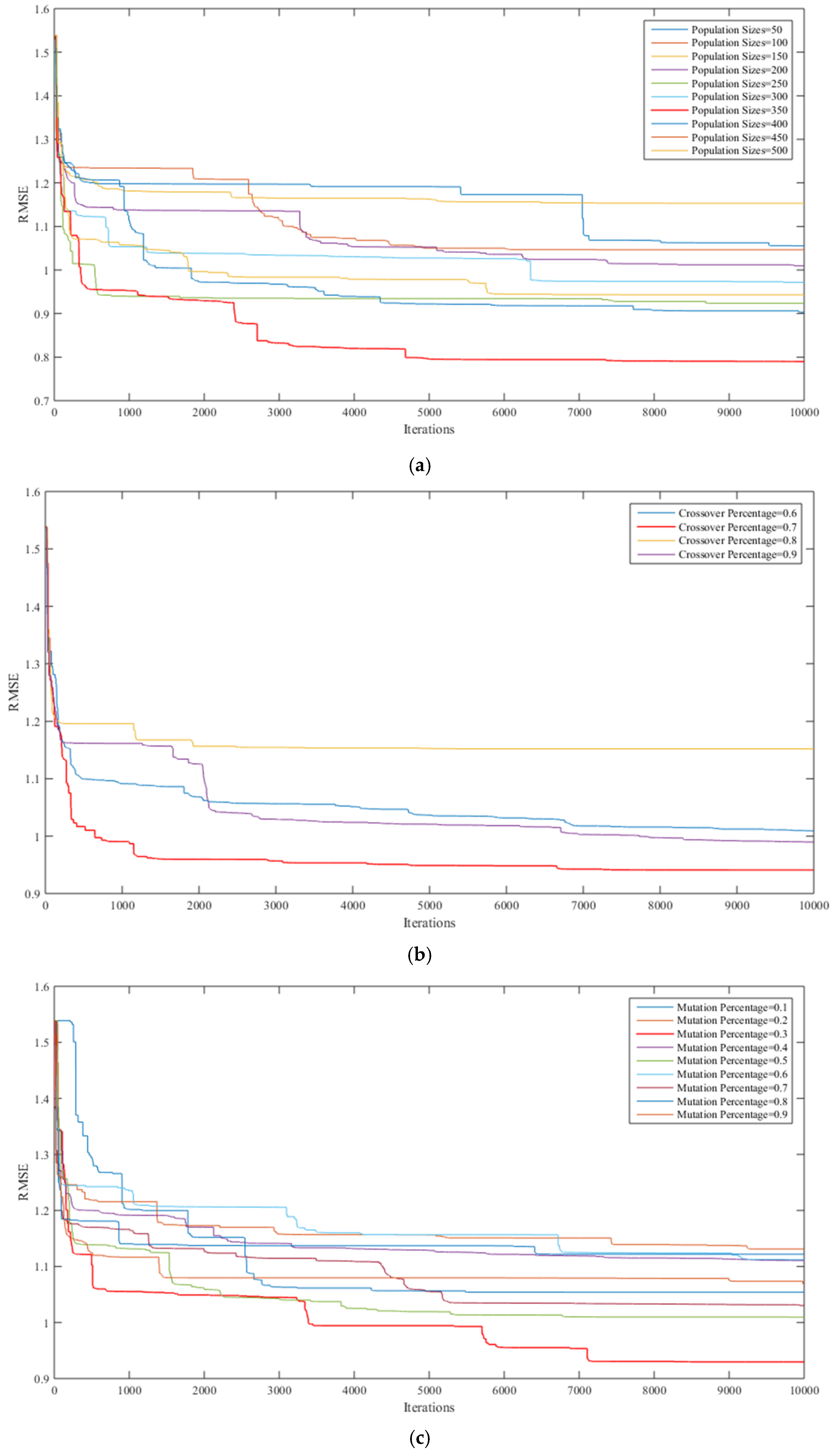
4.2. The Optimal Parameter of HM-GA

To obtain the optimized structure of HM-GA model, the influencing parameters, such as population size, crossover percentage, and mutation percentage, are changed to find the suitable structure, as shown in Figure 4a,c. The root mean square error is applied to measure the applicability of the optimum parameters.

From Figure 4a, the population sizes are changed in a range between 50 and 500, presented in 10 different colors. The red line gives the smallest RMSE value and reaches stability after 5000 iterations. Thus, the proper population size is examined at 350. A crossover percentage with a population size of 350 is varied in a range between 0.6 and 0.9, as shown in Figure 4b and indicated with four different colors. It can be clearly seen that the red line shows the smallest RMSE value. Hence, the crossover percentage of 0.7 is the appropriate case for this study. Simultaneously, a mutation percentage with population size of 350 and crossover percentage of 0.7 is considered in the range between 0 and 1, as shown in Figure 4c and displayed with nine different colors. At a mutation percentage of 0.3, the red line shows the experimental results providing the smallest RMSE value. As mentioned in these figures, it can be summarized that, for the HM-GA model, a population size equal to 350, crossover percentage equal to 0.7, and mutation percentage equal to 0.3 leads to the best predictive network in moisture predicting for the talc pellet forming process.

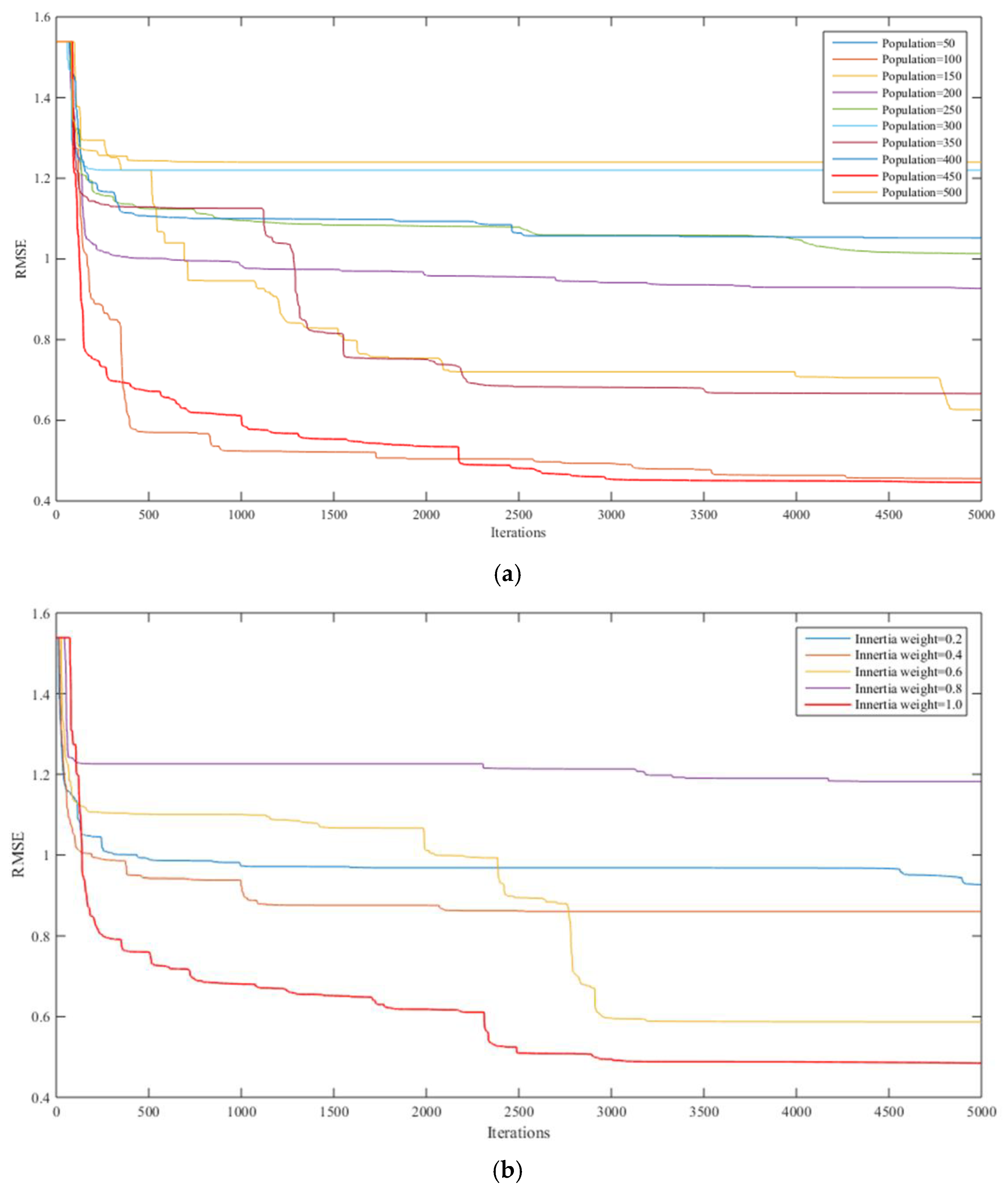
4.3. The Optimal Parameter of HM-PSO

The optimal parameter can increase the reliability of the model. For HM-PSO, the important parameters of PSO were assessed using a trial and error process. The different values of population sizes and inertia weight are investigated.

As in Figure 5a, 10 different cases of population size varied from 50 to 500 for iterations are presented. In Figure 5b, the inertia weight changed from 0.2 to 1 by a step of 0.2 for 5000 iterations are examined. From these figures, it can be concluded that, for the HM-PSO model, a population size equal to 450 and an inertia weight equal to 1.0 can lead to the best predictive network.

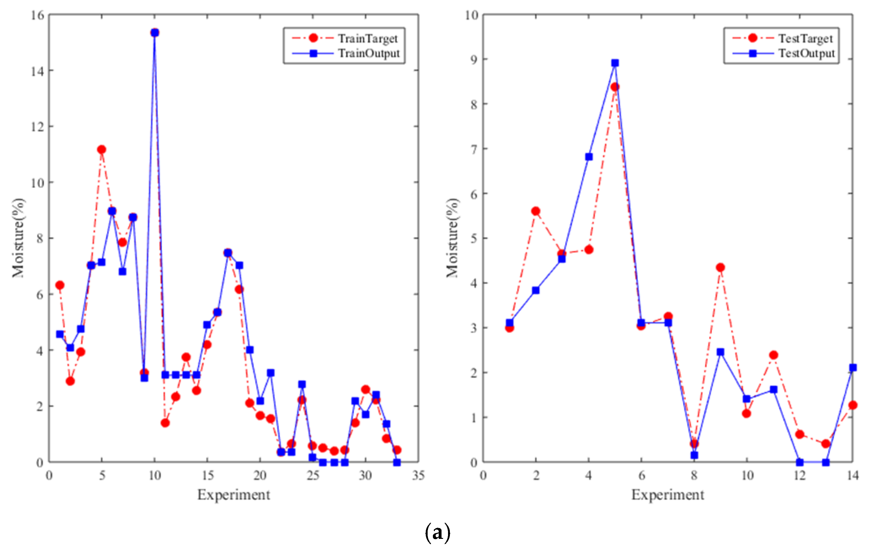
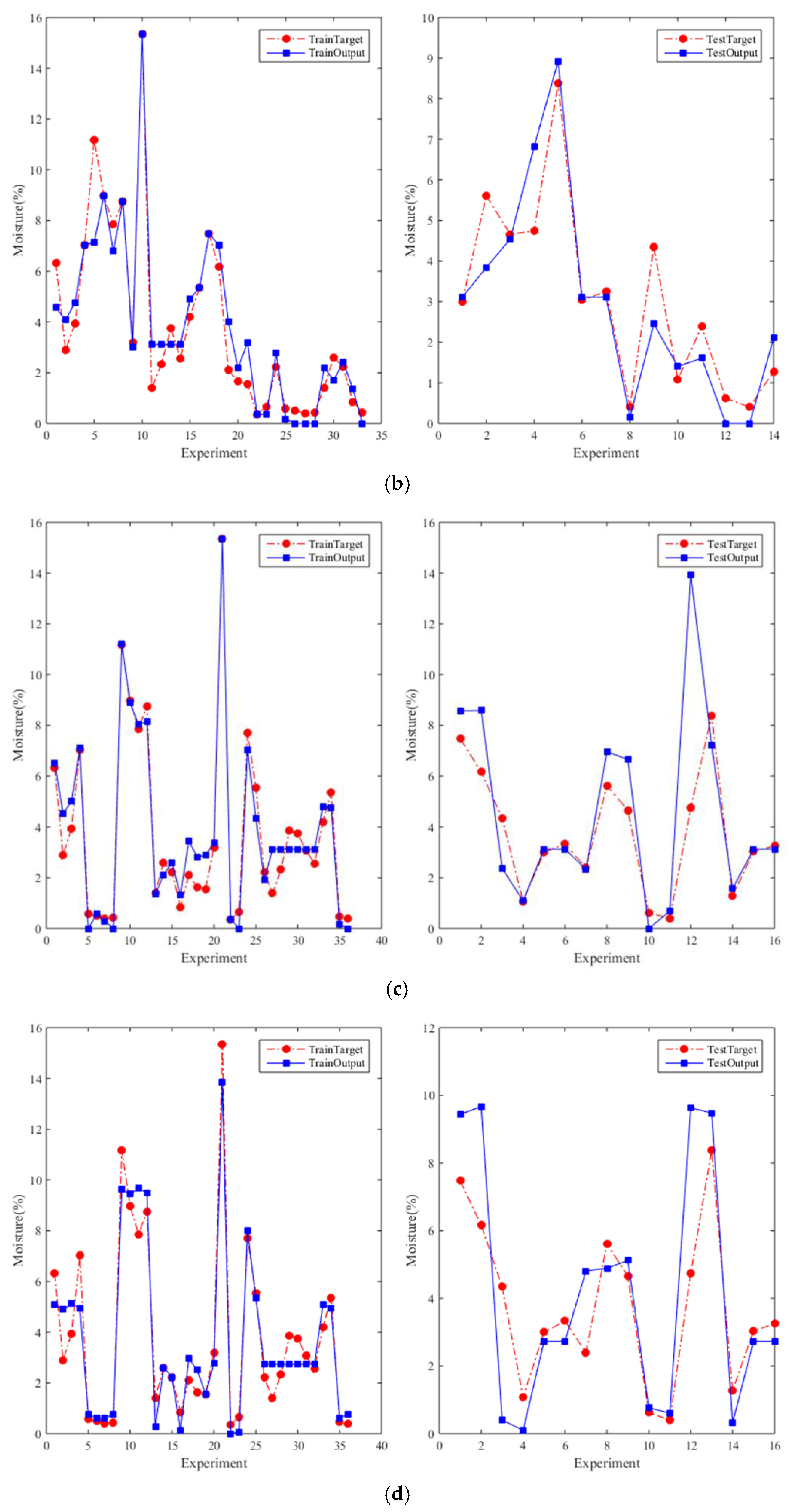
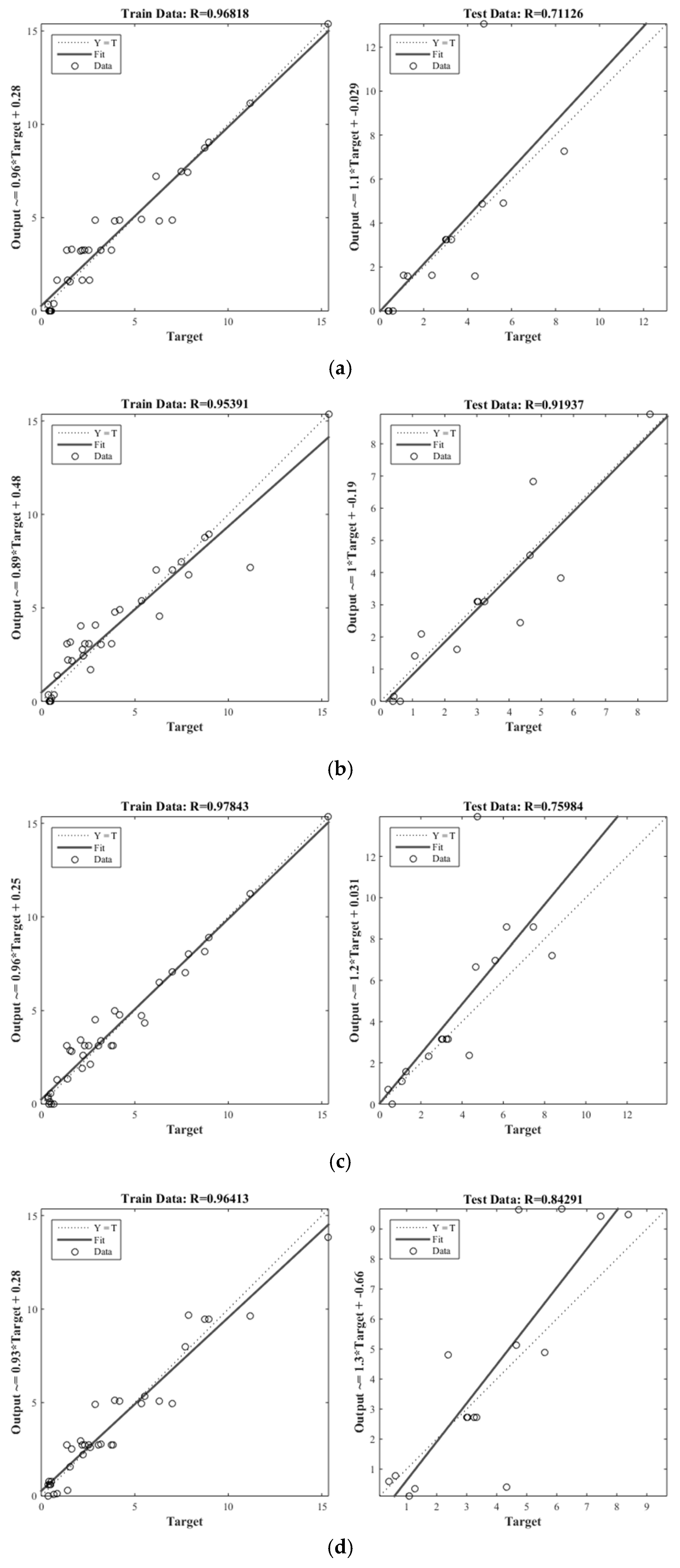
4.4. The Comparison Results Approach from HM-GA and HM-PSO

In order to predict the moisture in the talc pellet process, SOM is applied to select the appropriate input data and then the data are fed into ANFIS. The GA and PSO are chosen as training methods. As mentioned in Section 4.2, the optimal population size, crossover percentage, and mutation percentage of HM-GA and ANFIS-GA are 350, 0.8, and 0.6, respectively. As in Section 4.3, the optimal population size and inertia weight of HM-PSO and ANFIS-PSO are 450 and 1.0, respectively. To compare the performance of the proposed HM-GA and HM-PSO model, the ANFIS model without clustering trained by GA and PSO is examined, namely, ANFIS-GA and ANFIS-PSO. Table 6 shows the comparison of the performance between four models of HM-GA, HM-PSO, ANFIS-GA and ANFIS-PSO.

From Table 6, in the process of creating a model generated by the training dataset, ANFIS-GA has the highest R of 0.9784, and the lowest RMSE and AAD of 0.7203 and 0.314, respectively. In the test process, the HM-PSO has the highest R of 0.9192, the lowest RMSE of 0.9785, and the lowest AAD of 0.376. The relationship between the target and predicted moisture is a strong positive association. The value of AAD is used to measure the average distance between each data point and the mean. As can be seen in Table 6, the HM-PSO model demonstrates the smallest different value of AAD between the training and test data. Meanwhile, other models have larger different values of AAD between the training and test data. It can be obviously seen that three indicators of the HM-PSO indicates a smaller difference in value to both the training and test data than others. Additionally, the convergence speed of HM-PSO is faster and the predictive values conform with the measured values than others. It can be concluded that the HM-PSO has the most reliable results in predicting moisture in the talc forming process. Figure 6 shows the difference between the target and output values of the training and testing datasets.

According to Figure 6, the variation between the predicted moisture and target moisture is displayed. The red line represents the target moisture and the blue line is the predicted moisture. In the training process of each experiment, two models with SOM perform more similarity than two other models without SOM, although all models provide a high correlation coefficient. Simultaneously, for testing process, it is clearly seen that there are many experiment cases of ANFIS-GA and ANFIS-PSO that are too different between the target and predicted moisture values. By using SOM, the differentiation can be reduced, as in Figure 6a,b. The correlation between the target and predicted moisture values is shown in Figure 7.

In Figure 7, the relationship between the target and predicted moisture of four models is performed. It can be seen that the predicted moisture of HM-PSO, Figure 7b, lies in a relatively straight line for both the training and test data. The R value obtained from the HM-PSO is close to 1, R = 0.9539 for training data and R = 0.9192 for test data. Regarding the model, HM-PSO is a representative model for moisture prediction in the talc forming process.

5. Conclusions

The hybrid model, based on a combination of SOM and ANFIS, is introduced as the proposed model for moisture prediction in the talc forming process in Uttaradit, Thailand. The GA and PSO algorithms are selected as the training algorithms of ANFIS. Five important factors—talc powder, water, temperature, feed speed, and airflow—affecting moisture in the talc pellet forming process were recognized and appropriate data were collected. In order to verify the proposed model, HM-GA, HM-PSO, ANFIS-GA, and ANFIS-PSO are compared. As a result, the HM-PSO model gives a high correlation coefficient for both training and test data with R = 0.9539 and R = 0.9192, respectively. Furthermore, HM-PSO still has a similar RMSE value for training and test data, of about 0.09. For other models, it has a rather large, different RMSE value between training and test data. Therefore, HM-PSO performs more reliably compared to the other algorithms. Since it is a real-world problem occurring in Uttaradit, Thailand, no one applies this method to the talc pellet process. The results, therefore, cannot compare with earlier research. The HM has some limitations according to the optimal parameters: It is only suitable for this study. For other real-world problems, it is necessary to identify the optimal parameters of HM. In this study, it can be said that the idea of raw data management by using SOM to identify a similar group of data is very helpful to obtain the most significantly information to feed into ANFIS. This can reduce the computation time during the training process. The method with clustering can improve the prediction skill compared to the method without clustering, efficiently. For further study, more clustering methods, such as k-means, and more ANFIS training algorithms, such as bee colony or ant colony optimization, should be applied and compared with this study.

References

1. Driscoll, M. The structure of the Talc supply market. In Proceedings of the 3rd China Liaoning International Magnesia Materials Exposition, Shenyang, China, 22–24 September 2008; pp. 1–7. [Google Scholar]
2. Loveday, A.U.; Nwanya, S.C.; Amaechi, O.P. Artificial neural network application to a process time planning problem for palm oil production. Eng. Appl. Sci. Res. 2020, 47, 161–169. [Google Scholar]
3. Talpur, N.; Salleh, M.N.; Hussain, K.; Ali, H. Modified ANFIS with Less model complexity for classification problems. In Proceedings of the Computational Intelligence in Information Systems Conference (CIIS 2018), Phuket, Thailand, 17–19 November 2018; pp. 36–47. [Google Scholar]
4. Buragohain, M. Adaptive Network Based Fuzzy Inference System (ANFIS) as a Tool for System Identification with Special Emphasis on Training Data Minimization. Ph.D. Thesis, Indian Institute of Technology Guwahati, Guwahati, India, July 2008. [Google Scholar]
5. Caydas, U.; Hascalik, A.; Ekici, S. An Adaptive Neuro-Fuzzy Inference System (ANFIS) model for wire-EDM. Expert Syst. Appl. 2009, 36, 6135–6139. [Google Scholar]
6. Zhange, Y.; Lei, J. Prediction of laser cutting roughness in intelligent manufacturing mode based on ANFIS. Procedia Eng. 2017, 174, 82–89. [Google Scholar] [CrossRef]
7. Sen, B.; Mandal, U.K.; PrasadMondal, S. Advancement of an intelligent system based on ANFIS for predicting machining performance parameters of inconel 690—A perspective of metaheuristic approach. Measurement 2017, 109, 9–17. [Google Scholar] [CrossRef]
8. Abdollahi, H. An Adaptive Neuro-Based Fuzzy Inference System (ANFIS) for the prediction of option price: The case of the Australian option market. Int. J. Appl. Math. Comput. 2020, 11, 99–117. [Google Scholar] [CrossRef]
9. Bui, D.T.; Khosravi, K.; Li, S.; Shahabi, H.; Panahi, M.; Singh, V.; Chapi, K.; Shirzadi, A.; Panahi, S.; Chen, W.; et al. New hybrids of ANFIS with several optimization algorithms for flood susceptibility modeling. Water 2018, 10, 1210. [Google Scholar]
10. Yaseen, Z.M.; Ebtehaj, I.; Bonakdari, H.; Deo, R.; Mehr, A.D.; Mohtar, W.M.; Diop, L.; Ei-shafie, A.; Singh, V. Novel approach for streamflow forecasting using a hybrid ANFIS-FFA model. J. Hydrol. 2017, 554, 263–276. [Google Scholar] [CrossRef]
11. Gocken, M.; Boru, A. Integrating metaheuristics and ANFIS for daily mean temperature forecasting. Int. J. Glob. Warm. 2016, 9, 110–128. [Google Scholar] [CrossRef]
12. Oliverira, M.V.; Schirru, R. Applying particle swarm optimization algorithm for tuning a neuro-fuzzy inference system for sensor monitoring. Prog. Nucl. Energy 2009, 51, 177–183. [Google Scholar]
13. Alarifi, I.M.; Nguyen, H.M.; Bakhtiyari, A.N.; Asadi, A. Feasibility of ANFIS-PSO and ANFIS-GA models in predicting thermophysical properties of Al2O3-MWCNT/Oil hybrid nanofluid. Materials 2019, 12, 3628. [Google Scholar] [CrossRef] [Green Version]
14. Kumar, R.; Hynes, N.R. Prediction and optimization of surface roughness in thermal drilling using integrated ANFIS and GA approach. Eng. Sci. Technol. Int. J. 2020, 23, 30–41. [Google Scholar] [CrossRef]
15. Rezakazemi, M.; Dashti, A.; Asghari, M.; Shirazian, S. H2-selective mixed matrix membranes modeling using ANFIS, PSO-ANFIS, GA-ANFIS. Int. J. Hydrogen Energy 2017, 42, 15211–15225. [Google Scholar] [CrossRef]
16. Sabeti, M.; Deevband, M.R. Hybrid evolutionary algorithms based on PSO-GA for training ANFIS structure. Int. J. Comput. Sci. 2015, 12, 78–86. [Google Scholar]
17. Dariane, A.B.; Azimi, S. Forecasting streamflow by combination of genetic input selection algorithm and wavelet transform using ANFIS model. Hydrol. Sci. J. 2016, 61, 585–600. [Google Scholar] [CrossRef]
18. Jeong, C.; Shin, J.-Y.; Kim, T.; Heo, J.-H. Monthly precipitation forecasting with a neuro-fuzzy model. Water Resour. Manag. 2012, 26, 4467–4483. [Google Scholar] [CrossRef]
19. Kohonen, T.; Simula, O.; Visa, A.; Kangas, J. Engineering applications of the self-organizing map. Proc. IEEE 1996, 84, 1358–1384. [Google Scholar] [CrossRef]
20. Khanzadeh, M.; Rao, P.; Jafari-Marandi, R.; Smith, B.K.; Tschopp, M.A.; Bian, L. Quantifying geometric accuracy with unsupervised machine learning: Using self-organizing map on fused filament fabrication additive manufacturing parts. J. Manuf. Sci. Eng. 2018, 140, 1–12. [Google Scholar] [CrossRef] [Green Version]
21. Jha, R.; Dulikravich, G.S.; Chakraborti, N.; Fan, M.; Schwartz, J.; Koch, C.C.; Marcelo, J.; Colaco, M.J.; Poloni, C.; Egorov, I.N. Self-organizing maps for pattern recognition in design of alloys. Mater. Manuf. Processes 2017, 32, 1067–1074. [Google Scholar] [CrossRef]
22. Nourani, V.; Alami, M.T.; Vousoughi, F.D. Hybrid of SOM-clustering method and wavelet-ANFIS approach to model and infill missing groundwater level data. J. Hydrol. Eng. 2016, 21, 1–19. [Google Scholar] [CrossRef]
23. Amiryousefi, M.R.; Mohebbi, M.; Khodaiyan, F.; Asadic, S. An empowered adaptive neuro-fuzzy inference system using self-organizing map clustering to predict mass transfer kinetics in deep-fat frying of ostrich meat plates. Comput. Electron. Agric. 2011, 76, 89–95. [Google Scholar] [CrossRef]
24. Nasir, V.; Cool, J. Intelligent wood machining monitoring using vibration signals combined with self-organizing maps for automatic feature selection. Int. J. Adv. Manuf. Technol. 2020, 108, 1811–1825. [Google Scholar]
25. Standard Test Method for Laboratory Determination of Water (Moisture) Content of Soil and Rock by Mass; ASTM D 2216–98; ASTM International: Washington, DC, USA, 28 March 2004.
26. Asan, U.; Ercan, S. An Introduction to Self-Organizing Maps; Atlantis Press: Istanbul, Turkey, 2012; pp. 299–319. [Google Scholar]
27. Wangsoh, N.; Watthayu, W.; Sukawat, D. Appropriate learning rate and neighborhood function of Self-Organizing Map (SOM) for specific humidity pattern classification over Southern Thailand. Int. J. Model. Optim. 2016, 6, 61–65. [Google Scholar]
28. Stefanovic, P.; Kurasova, O. Visual analysis of Self-Organizing Maps. Nonlinear Anal. 2011, 16, 488–504. [Google Scholar] [CrossRef] [Green Version]
29. Jang, J.-S.R. ANFIS: Adaptive-Network-Based Fuzzy. IEEE Trans. Syst. Man Cybern. Syst. Hum. 1993, 23, 665–685. [Google Scholar]
30. Holland, J. Adaptation in Natural and Artificial Systems: An Introductory Analysis with Applications to Biology, Control and Artificial Intelligence; MIT Press: Cambridge, MA, USA, 1979. [Google Scholar]
31. Goldberg, D.E. Genetic Algorithm in Search Optimization and Machine Learning; Addison Wesley: Boston, MA, USA, 1989. [Google Scholar]
32. Kennedy, J.; Eberhart, R.C. A new optimizer using particle swarm theory. In Proceedings of the Sixth International Symposium on Micromachine and Human Science, Nagoya, Japan, 4–6 October 1995; pp. 39–43. [Google Scholar]
33. Talukder, S. Mathematical Modelling and Applications of Particle Swarm Optimization. Master’s Thesis, Blekinge Institute of Technology, Karlskrona, Sweden, February 2011. [Google Scholar]
34. Ohale, P.E.; Uzoh, C.F.; Onukwuli, O.D. Optimal factor evaluation for the dissolution of alumina from azaraegbelu clay in acid solution using RSM and ANN comparative analysis. S. Afr. J. Chem. Eng. 2017, 24, 43–54. [Google Scholar] [CrossRef]
35. Montogomery, D.C. Design and Analysis of Experiments; John Wiley & Sons Inc.: New York, NY, USA, 2001. [Google Scholar]
36. Pham, H. Springer Handbook of Engineering Statistics; Springer: London, UK, 2006. [Google Scholar]
37. Moayedi, H.; Raftari, M.; Sharifi, A.; Jus, W.W.; Safuan, A.; Rashid, A. Optimization of ANFIS with GA and PSO estimating α ratio in driven. Eng. Comput. 2019, 36, 227–238. [Google Scholar] [CrossRef]
38. Wu, D.; Chen, H.; Huang, Y.; He, Y. Monitoring of weld joint penetration during variable polarity plasma arc welding based on the keyhole characteristics and PSO-ANFIS. J. Mater. Process. Technol. 2017, 239, 113–124. [Google Scholar] [CrossRef]
39. Lei, S.; Zhan, H.; Wang, K.; Su, Z. How training data affect the accuracy and robustness of neural networks for image classification. In Proceedings of the International Conference on Learning Representations, New Orleans, LA, USA, 6–9 May 2019; pp. 1–14. [Google Scholar]
40. Ismail, S.; Shabri, A.; Samsudin, R. A hybrid model of Self Organizing Maps and least square support vector machine for river flow forecasting. Hydrol. Earth Syst. Sci. 2012, 16, 4417–4433. [Google Scholar]
Figure 1. Talc pellet forming process.
Symmetry 12 01602 g001
Figure 2. An architecture of ANFIS [12].
Symmetry 12 01602 g002
Figure 3. The schematic HM for moisture prediction in the talc forming process.
Symmetry 12 01602 g003
Figure 4. The optimal parameter of GA algorithm: (a) population size; (b) crossover percentage; (c) mutation percentage.
Symmetry 12 01602 g004
Figure 5. The optimal parameters of the PSO algorithm: (a) population size; (b) inertia weight.
Symmetry 12 01602 g005
Figure 6. The difference between the target and predicted moisture: (a) HM-GA; (b) HM-PSO; (c) ANFIS-GA; (d) ANFIS-PSO.
Symmetry 12 01602 g006aSymmetry 12 01602 g006b
Figure 7. The correlation between the target and predicted moisture: (a) HM-GA; (b) HM-PSO; (c) ANFIS-GA; (d) ANFIS-PSO.
Symmetry 12 01602 g007