1. Introduction
The Fornberg–Whitham equation
appeared in the study of qualitative behaviors of wave-breaking [
1,
2]. In [
3], Fornberg and Whitham obtained a peak solution of the form
for Equation (
1). We can see the similarity between Equation (
1) and the well-known Camassa–Holm equation
If
, then Equation (
2) has the peakon solution
[
4]. If
, then Equation (
2) has the peakon solution
[
5]. In addition to the distinction in the coefficients, there exists a great difference, i.e., for
, Equation (
2) possesses the property of complete integrability and bi-Hamiltonian structure while Equation (
1) does not have such advantage [
6].
Since the appearance of the Camassa–Holm equation Equation (
2), a huge amount of work has been carried out to study the dynamic properties of Equation (
2). Equation (
2) has been proved to possess the global existence, the precise blow-up scenario, the blow-up set and the blow-up rate for the strong solutions [
7,
8,
9,
10]. It has also been confirmed that the peakon of Equation (
2) are orbitally stable [
11,
12].
In [
13], Liu and Qian suggested a generalized Camassa–Holm equation
Similarly, by softening the nonlinear term, He et al. [
14] studied the peakons and solitary waves for the modified Fornberg–Whitham equation
However, little attention has been given to the periodic traveling wave solutions in their study.
Recently, periodic traveling waves of nonlinear equations have received great attention. For instance, Angulo et al. [
15] mentioned that the cnoidal waves of KdV equation converge to the limit soliton when the period tends to infinity. The detailed study was presented by Neves [
16]. In [
17], the periodic asymptotics of a class of stationary nonlinear Schrödinger equations has been studied together with the existence of dark soliton. The authors [
18] showed that the limit forms of the periodic loop solutions of the Kudryashov–Sinelshchikov equation contained loop soliton solutions, smooth periodic wave solutions, and periodic cusp wave solutions.
In this paper, we study the explicit periodic wave solutions and their asymptotic property for Equation (
4) using bifurcation analysis [
19,
20,
21,
22,
23,
24,
25,
26]. Also, some periodic wave solutions are symmetric [
27]. First, we obtain two types of explicit periodic wave solutions, elliptic smooth periodic wave solutions and periodic blow-up solutions with a parameter
. Secondly, we reveal that there exist four parametric values. When
tends to these parametric values, these elliptic periodic wave solutions can become other three types of nonlinear wave solutions, the hyperbolic smooth solitary wave solutions, the hyperbolic blow-up solutions and the trigonometric periodic blow-up solutions.
This paper is organized as follows. In
Section 2, we give some preliminaries. Our main results are listed in
Section 3. In
Section 4, we provide derivation to our main results. A short conclusion is given in
Section 5.
2. Preliminaries
To derive our results, we give some preliminaries in this section. For given constant c, substituting
with
into Equation (
4), it follows that
Integrating (
5) once, we have
where
g is an integral constant. Letting
, we get a planar system
with the first integral
where
h is another integral constant.
Assuming that
and
c (double root) are two real roots of the equation
we get its other two roots
and
of forms
and
Solving equations
,
, and
respectively, we get the four numbers
of forms
where
From above expressions we get the following lemma.
Lemma 1. To make σ real, denote , , when constant wave velocity , there are the following facts.
(1) , , and are real and satisfy inequality (2) If or , then β and γ are complex. If , then β and γ are real and there exists the following properties.
(i) When , it follows that (ii) When , it follows that (iii) When , it follows that (iv) When , it follows that (v) When , it follows that (vi) When , it follows that (vii) When , it follows thatAccording to the above inequalities, we give some notations as follows:Using above these notations, on the φ-y plane we obtain some special points , , . Via (2.4) we display the orbits passing these special points as Figure 1. 3. Our Main Results
In this section, we state our main results. The pictures of Proposition 1 are included in the
Appendix A.
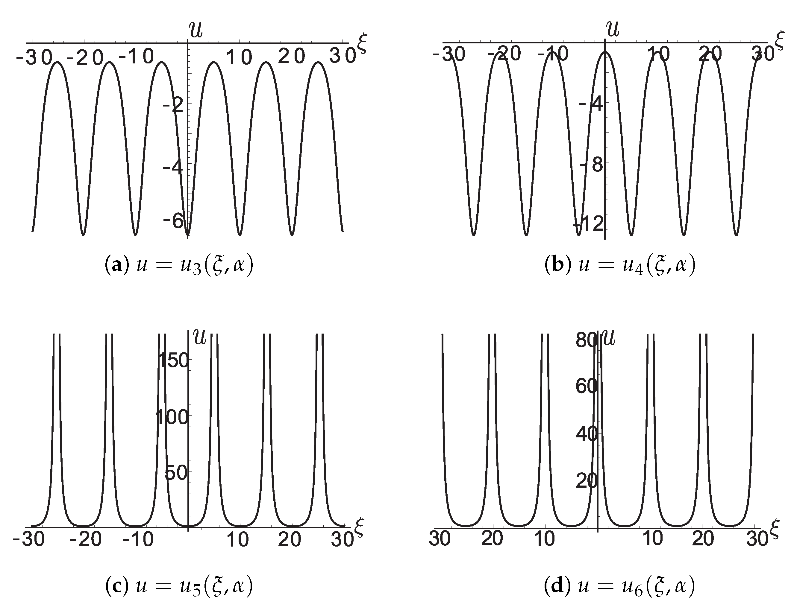
Proposition 1. For given and arbitrary real number α, if letand β, γ be in (10)–(11), and be in (12)–(15), then Equation (4) has the following explicit periodic wave solutions. (1) If
or
, then the explicit periodic wave solutions are
and
where
and
For the graphics of
and
with
and
, see
Figure A1a,b.
These two solutions possess the following limits.
When
,
becomes the trigonometric periodic blow-up solution
and
becomes the trigonometric periodic blow-up solution
When
,
becomes the smooth solitary wave solution
and
becomes the hyperbolic single blow-up solution
For the varying figures of
when
, and
where
, see
Figure A2a–c. For the varying figures of
when
,
and
, see
Figure A3a–c.
(2) If
satisfies
and
, then the explicit periodic wave solutions are
and
where
and
,
,
are in (
25)–(
27).
For the figures of
with
and
, see
Figure A4a–d.
These four solutions possess the following limits.
When
or
, the smooth periodic wave solutions
and
become the trivial solution
, and the elliptic periodic blow-up solutions
,
respectively become the trigonometric periodic blow-up solution
and
given (
36) and (
37).
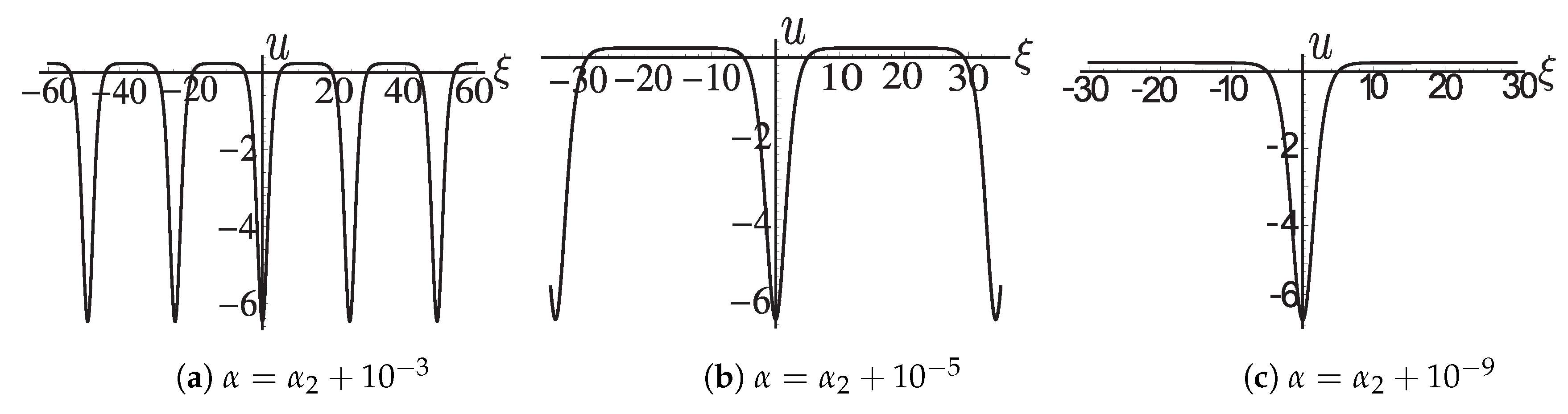
When
or
, the smooth periodic wave solution
becomes the smooth solitary wave solution
given in (
38), the smooth periodic wave solution
and the periodic blow-up solution
become the trivial solution
, and the elliptic periodic blow-up solution
becomes the hyperbolic single blow-up solution
given in (
39). For the varying figures of
when
,
and
, see
Figure A5a–c. For the varying figures of
when
,
and
, see
Figure A6a–c.
4. The Derivation of Main Results
In this section, we give the derivation for our main results listed in Proposition 1. First, we derive and their limit forms.
(1) If
or
, then via Lemma 1 we know that Equation (
9) has four roots
c,
,
and
. The root c is a double real root.
is a simple real root.
and
are two complex roots. From
Figure 1a we see that on
plane there is an open orbit
passing the point
. The open orbit
possesses expression
where
and
are given in (
34) and (
35).
Substituting (
46) into
and integrating it along
, we have
and
Completing the integral in (
47) and (
48), we get
and
where
and
are listed in (
31) and (
32). Respectively solving Equation (
49) and Equation (
50) for
and noting that
, we obtain
and
of forms (
29) and (
30).
Since the period of the function
is 4K, where
This completes the derivations of
.
Now we show the limits of as or .
() When
, it follows that
which implies that
,
and
.
This implies that the property is true.
() When
, it follows that
which implies that
,
and
.
Thus, we have
Further it follows that
and
This implies that the property
holds.
Secondly, we derive and their limit forms.
(2) If
and
,
, then from Lemma 1 we see that Equation (
9) has four real roots
c,
,
and
. The root
c is a double real root. The other three roots are simple real roots. From the expressions (
25)–(
27) of
,
,
and
Figure 1b, we can see that there exists a closed orbit
passing the points
,
, and there is an open orbit
passing
on
plane. The closed orbit
possesses expression
and the open orbit
has expression
Substituting the above two expressions into
and integrating it along the two orbits, we have
and
Completing the above four integrals, the four equations respectively become
and
where
is given in (
44). Solving the above four equations for
respectively and noting that
, we get the solutions
of the forms (
40)–(
43).
Since the period of the function is , it follows that the period of the function is .
Now we derive the limit forms. First, we derive the limit forms
. From the expressions (
25)–(
27), we have the following limits.
(i) When
, it follows that
(ii) When
, it follows that
(iii) When
, it follows that
Thus, when
or
, we have
and further have
and
These complete the derivations for limit forms
.
Secondly, we derive the limit forms
. Similarly, from (
25)–(
27) we get the following limits.
(iv) When
, we have
(v) When
, we have
(vi) When
, it follows that
Thus, when
or
, we have
and further have
and
Hereto we have finished the derivations for our main results.
5. Conclusions
In this paper, we have studied the explicit smooth periodic wave solutions and periodic blow-up solutions and their asymptotic property for Equation (
4). In Proposition 1, the explicit expressions of these solutions and their limits have been shown. Based on these results, Equation (
4) possesses explicit periodic wave solutions, and solitary wave solution has been exposed. Furthermore, we have found that the periodic blow-up solution
can converge to the smooth solitary wave solution
. On the other hand, this example shows that not only the cnoidal wave solution but also the periodic blow-up solution can converge to the smooth solitary wave solution.
Furthermore, a new phenomenon about the periodic solution has been discovered. In [
16], the author proved that when the period tends to
∞, the cnoidal waves of KdV equation, on compact sets, converge to the limit soliton. In our paper, it has been found that when the period
tends to
, the elliptic periodic blow-up solutions
and
become the trigonometric periodic blow-up solution
and
respectively. Also, when the period
tends to
,
and
become
and
respectively.
Finally, the correctness of all the solutions are also validated by the mathematical software.


