Padé and Post-Padé Approximations for Critical Phenomena

Abstract

We discuss and apply various direct extrapolation methods for calculation of the critical points and indices from the perturbative expansions my means of Padé-techniques and their various post-Padé extensions by means of root and factor approximants. Factor approximants are applied to finding critical points. Roots are employed within the context of finding critical index. Additive self-similar approximants are discussed and $DLog$ additive recursive approximants are introduced as their generalization. They are applied to the problem of interpolation. Several examples of interpolation are considered.

1. Introduction

We address an old and important problem of extrapolating asymptotic expansions in powers of a small variable to large values of the variable [1]. It is very often confronted in various disciplines of natural science and applied mathematics. Of course, one would like to have an exact solution to a realistic problem. But such problems are too complicated, and do not allow to obtain exact solutions. Most often one would try to develop some kind of a perturbation theory [2,3]. Then, the sought quantities are given in the forms of most often divergent expansions. More precisely, expressed as truncated series in powers of a small positive parameter, say x, as $x\to 0$. Out task is to recast such divergent series, into convergent expressions by means of analytical constructs called approximants.

The main difficulty arises because the problem of interest pertains not to a small variable, but to a large values of this variable. In the most extreme scenario it is the infinite limit, as $x\to \infty$, that should be found. In practice, only several expansion terms can be derived. And the resulting asymptotic series are divergent. The hard problem consists in reconstructing from the several terms of an asymptotic expansion as $x\to 0$ completely different limit as $x\to \infty$.

The variable $x>0$ can represent some practically important situations. It can be a coupling constant in field theory, or concentration of particles in composites. Based on the same asymptotic material, such as series coefficients, thresholds, critical indices, correction to scaling indices one can construct not only Padé but also post-Padé approximations. The list of such approximants is not complete or finished by any means. It includes tentatively Padé, $Log$-Padé, $DLog$-Padé, factor, root, corrected Padé, additive, $DLog$-additive approximants etc.

In a more rigorous terminology, we are interested in the behavior of a real function $\Phi (x)$ of a real variable $x\in \left[0,\infty \right)$. Let this function be the solution to some complicated problem. And the problem would not allow for an explicit knowledge of the function. In order to solve such problem we sometimes manage to come up with some perturbation theory. The theory yields asymptotic expansions about $x=x_0=0$,

$$\Phi (x)\sim \sum _{n=0}^{\infty }{c}_n{x}^n.$$

(1)

One often extrapolates small-variable expansions by means of Padé approximants denoted as $P_{M,N}(x)$ [4]. Straightforward application of these approximants yields asymptotic behavior which depends on the concrete values of M and N. The Padé approximant can tend to either infinity, to zero, or to a constant. In that sense, the limit $x\to \infty$ is not well-defined. One would like to reduce the uncertainty. To this end we can agree to prefer the diagonal Padé approximants over other alike sequences. The method of corrected approximants allows to accomplish such task [5,6]. It is also ill-advised to forgo the well developed techniques of Padé approximants. The corrected Padé approximants are applicable the problems indeterminate from the view point of a standard Padé approximants [6,7]. The technique will be applied extensively in the Section 3.

One can think that the idea of corrected approximants [6,7,8], is going to have the advantage over all other techniques, because it permits to combine the strength of a few methods together. Then, in the space of approximations, one can proceed with piece-wise construction of the approximation sequences. In [5,6], we observe that technique can solve some hard problems by combined application of the two approximation methods, even when each of them separately failed.

In a nutshell, the Padé approximant $P_{M,N}$ to an analytical function $\Phi (x)$ at a regular point $x=x_0=0$ is the ratio of two polynomials of the degree M and of the degree N. The approximant with $M=N$ plays often a central role in various studies. It is called a diagonal Padé approximant of order N.

The beauty of Padé approximants is striking. The coefficients of the approximants can be derived explicitly from the coefficients of the given power series from the solution of a linear system of equations. To this end we impose the requirement of asymptotic equivalence to the given series (1), representing the sought function $\Phi (x)$. The poles of Padé approximants determine singular points of the sought functions [4]. But the functions in the vicinity of their critical points, in general, are non-rational. Therefore the direct use of Padé approximants for finding critical behavior is impossible.

Often, in addition to the expansion about $x=x_0=0$, an additional information is available. It is contained in the expansion about $x=\infty$,

$$\Phi (x)\sim \sum _{n=0}^{\infty }{b}_n{x}^{-n}.$$

(2)

A two-point Padé approximant to $\Phi (x)$ is a rational function constructed in such a manner that both asymptotic forms, (1) and (2) are satisfied. More can be learned from the comprehensive books [4,9].

However the accuracy of the two-point Padé approximants is not high. Moreover it confronts several real difficulties [7,8]. The standard situation in many problems is when for small x one has an expansion in integer powers, $x^n$, and for the large-variable expansion exhibits the behaviour with a non-integer power $\beta$. To overcome the problem of incompatibility of the Padè techniques, Baker and Gammel [10], used the fractional powers of Padé approximants. The simplest case of the Baker–Gammel method is the polynomial approximant in a fractional power. See also [1] for similar modification to the Padé approximants. Still, even the Baker–Gammel approximants represent correctly only the leading term of the large-variable behaviour.

One should also remember about the optimized perturbation theory [11,12]. It is based on the technique of optimization with special techniques for introducing control functions. Within the framework of the variational perturbation theory [13], the control functions are introduced differently. One has to consider special variable transformation with optimization parameter. Subsequently, variational optimization conditions are imposed.

The self-similar approximation theory developed by V. I. Yukalov and L. P. Yukalova in 1990–1996, can be used without introducing control functions, which makes calculations essentially simpler (see e.g., [7] for extensive references). See also the review [14], where notion of self-similarity is comprehensively discussed. Wildly successful and popular method of renormalization group in quantum filed theory and phase transitions [2,15], is based on improvements to a perturbative expansions by uncovering or imposing self-similarity. Ironically, celebrated $ϵ$-expansion for the critical indices [15], appeared to be asymptotic and require resummation by themselves, see e.g., [16]. The so-called super-exponential approximants give rather good resummation results for all spatial dimensions and number of components of the order parameter [16].

Various approximants employed in the present paper were obtained by same principle, by employing the asymptotic expansions and self-similarity imposed in the space of approximations [17].

Even when just a few coefficients in the expansion are known the above mentioned methods provide reasonable accuracy. For instance, equations of state can be derived in two and three dimensions, complying well with the experimental data [8]. Asymptotic approaches and interpolation with Padé and modified Padé approximants are successfully and extensively employed in mechanics and aerodynamics [18,19].

In our brief introduction, we tried no to repeat, to the best of our ability, some well-known facts and formulas, unless it was absolutely necessary. They are extremely well presented in treatises by Baker, Bender, Andrianov and Awrejcewicz with colleagues.

Nevertheless, some current developments in the field still need elaboration. Hence, the current paper. The paper should not be taken for a pure mathematical research (or review). In fact, it is a collection of practical recommendations, intended to advice how to use various results obtained in the mathematical theory of approximations in various practical contexts. We believe such recommendations are important for people working in applied science. Wherever it is possible we separate rigorous mathematical facts and mathematical definitions from a more informal discussion suggested for a reader interested in practical usage.

2. Ruina-Dieterich Model for Landslides and Factor Approximants. Critical Point

2.1. Factor Approximants

We follow [20,21,22] in the introduction of the self-similar factor approximants [20]. The k-th order factor approximant reads as follows

$${\Phi }_k^{*}(x)=\prod _{i=1}^{N_k}{(1+{\mathcal{P}}_{i}x)}^{n_i}.$$

(3)

The two cases, even and odd, could be separated,

$$\begin{array}{cc}{N}_k=\frac{k}{2},\hfill & k=2,4,\dots \hfill \\ N_k=\frac{k+1}{2},\hfill & k=3,5,\dots .\hfill \end{array}$$

(4)

The parameters ${\mathcal{P}}_i$ and $n_i$ typically are defined from the accuracy-through-order procedure. Such procedure consists in expanding the factor approximants in powers of x, and subsequent comparison of the latter expansion with the series (1). In the even case of $k=2p$, the procedure is uniquely defined and allows to compute all $2p$ parameters. In the odd case same additional condition should be imposed, either based on physical intuition, or computational expedience.

The factor approximants (3) can be used for identifying singularities when some ${\mathcal{P}}_i$ and $n_i$ are negative. It is possible to associate such singularities with critical points and critical indices of phase transitions [20].

2.2. Ruina-Dieterich Model

There is an understandable interest in understanding and (maybe) predicting catastrophic phenomena. Here, we discuss a simple model of landslides [23,24], which occur in a wide variety of geological and triggering processes.

We briefly recapitulate the main points of the discussion in [23,24]. The standard approach to slope instability is to find the conditions for a slope to become unstable. But the standard stability analysis cannot account for acceleration in slope movement. Such modeling strategy gives a nothing-or-all signal. It appears that any specific landslide is essentially unpredictable. Thus, one should focus on the recognition of landslide prone areas. This “time-independent hazard” approach essentially amounts to assumption that landslides are a random process in time. It uses geo-mechanical modeling to constrain the future long-term landslide hazard. In contrast,“time-dependent hazard” would assume a degree of predictability in the process. It is feasible that the landslide hazard varies with time.

The slider-block model takes into account the state-and-velocity-dependent friction, and was adjusted for studying landslides [23,24]. Mind that the factor approximants can be adapted for solving differential equations, nonlinear ODE in particular [22]. But the approach of [22] can be extended for analysis of singularities. Let us remind the main tenets of Ruina-Dieterich law of solid friction between two solid surfaces sliding against each other. The Ruina-Dieterich law involves the so-called state variable denoted here as F in a dimensionless form, which is usually thought to quantify the true area of contacts of the asperities of two solid surfaces. The state variable is just a different way to express the block velocity V. The two quantities are simply related, so that variable $V\propto \frac{1}{F^m},$ with positive parameter m.

The time evolution equation of the state variable of a block subjected to constant shear over normal stress, adheres to the Ruina-Dieterich solid friction law [25]. The state variable F obeys the following non-linear differential equation

$$\frac{dF}{dt}=b-F^{1-m}.$$

(5)

The law (5) results from a velocity-dependent solid friction coefficient, and and b and m stand for the parameters of the constitutive velocity-dependent solid friction law. Following to the [22,23,24], we derive from the Equation (5) the short-time expansion for $F(t)$. It is naturally represented as the series in powers of time t. In the equation studied in the paper [26] there is also an additional parameter $\alpha$ of the solid friction law. It can be safely excluded from consideration by simple re-scaling of the state variable and time and will be not included into the consideration.

We simply use the Taylor expansion formula and take a successive derivatives of (5), to obtain the following expansion

$$\begin{array}{c}F(t)\simeq a_0+a_{1}t+\frac{a_2{t}^2}{2!}+\frac{a_3{t}^3}{3!}+\frac{a_4{t}^4}{4!}+\frac{a_5{t}^5}{5!}+\frac{a_6{t}^6}{6!}+\frac{a_7{t}^7}{7!}+\frac{a_8{t}^8}{8!},\hfill \end{array}$$

(6)

with

$$\begin{array}{c}{a}_0=F(0),\hfill \\ a_1=b-F{(0)}^{1-m},\hfill \\ a_2=a_1(m-1){F(0)}^{-m},\hfill \\ a_3=(m-1){F(0)}^{-m-1}\left(a_{2}F(0)-{a_1}^{2}m\right),\hfill \\ a_4=(m-1){F(0)}^{-m-2}\left({a_1}^{3}m(m+1)-3a_1{a}_{2}F(0)m+a_3{F(0)}^2\right),\hfill \\ a_5=(m-1){F(0)}^{-m-3}(a_4{F(0)}^3-m({a_1}^4(m+1)(m+2)-6{a_1}^2{a}_{2}F(0)(m+1)+\hfill \\ 4a_1{a}_3{F(0)}^2+3{a_2}^2{F(0)}^2)).\hfill \end{array}$$

(7)

The coefficients $a_6,a_7,a_8$ become lengthy, but still easily manageable within the Mathematica. Consider the case of $a_1<0$. It corresponds to the solid friction state variable decrease from an initial large value. The parameters for the two different cases to be considered below are picked in order to reflect th existence of the two different regimes. In the relaxation scenario they correspond to a strong initial disequilibrium, obviously difficult case. Otherwise they are picked “almost” at random, and to describe the typical behaviour for each regime. Almost here means that for the regime with criticality studied below, the threshold and critical index by order of magnitude agree with the corresponding quantities of some Ising-type models of statistical physics [27]. Such choice allows in principle, to compare the accuracy achieved in computations with the same approximants. It appears that the accuracy is also of the same order for the two different models when treated with factor approximants [20,21].

2.2.1. Case of Relaxation Phenomena

In such case we are dealing with relaxation from some initial value to the constant determined by the system parameters. Consider first, the case $m<1$. Let $m=0.85$, $b=0.526$, and the initial condition, $F(0)=0.5$. Then,

$$\begin{array}{c}F(t)\simeq \frac{1}{2}-0.37525t+0.0507292t^2+0.00621518t^3+0.00113675t^4+0.000229336t^5\\ +0.0000435367t^6+5.586390517432677\times {10}^{-6}{t}^7-9.006206442078615\times {10}^{-7}{t}^8.\end{array}$$

(8)

There is also an additional condition, as $t\to \infty$. It reads simply,

$$F(t)\to b^{\frac{1}{1-m}}\equiv F_0.$$

Comparing $F(0)$ and $F_0$ one can see that they corresponds to the initial strong disequilibrium, as also clearly seen in Figure 1. In terms of the factor approximant of 4th order the solution is shown below,

$$\begin{array}{c}{F}_f^{*}(t)-F_0={\Phi }_4^{*}(t)=\\ 0.486199{(1-(0.385504+0.0708111i)t)}^{0.677165-1.76317i}\times \\ {(1-(0.385504-0.0708111i)t)}^{0.677165+1.76317i}\end{array}$$

(9)

The solution (9) is vastly superior to the two-point Padé approximant.

$$F_p^{*}(t)=\frac{1/2-0.454597t+0.107629t^2-4.353979016389374\times {10}^{-6}{t}^3}{1-0.158693t-0.00529935t^2-0.000315487t^3},$$

(10)

as shown in Figure 1.

Exponential-type approximations seems more natural in the considered regime, since it was shown that in along-time limit the equilibrium $F_0$ is being approached exponentially [26]. Thus, even more accurate solution could be obtained in terms of self-similar exponential approximants [16]. Their sequence rapidly converges in the 4th order to the approximant $F_{e,4}^{*}(t)$,

$$\begin{array}{c}{F}_{e,1}^{*}(t)-F_0=E_1^{*}(t)=0.486199e^{-0.771804t},\\ F_{e,2}^{*}(t)-F_0=E_2^{*}(t)=0.486199e^{-0.771804e^{0.250714t}t},\\ F_{e,3}^{*}(t)-F_0=E_3^{*}(t)=0.486199e^{-0.771804e^{0.250714e^{0.184395t}t}t},\\ F_{e,4}^{*}(t)-F_0=E_4^{*}(t)=0.486199e^{-0.771804e^{0.250714e^{0.184395e^{0.155074t}t}t}t}.\end{array}$$

(11)

It turned out recently that for relaxation phenomena one can apply the same elaborated techniques as for critical phenomena [28].

2.2.2. Case of Critical Behavior

We are more interested in critical behavior, supposedly describing the landslide [23,24]. It arises as the finite-time singularity solution, or moving singularity solution [9], to the Ruina-Dieterich law of solid friction (5). It is for $m>1$, that the solution can reach zero at the duration of a critical time $t_c$, which corresponds to the time when the catastrophic landslide is going to happen, since at this time block velocity becomes infinite. The critical point/time $t_c$ is approached with the critical index $1/m$. Let $m=1.5$ and keep all other parameters the same as for the noncritical case of the previous subsection. Mind that only a pure interpolation problem was studied in [29]. It did not involve any actual attempt to calculate the critical time or index, but only matches the two asymptotic regimes.

Based in the parameters of the problem, we can estimate that the critical time is $t_c=0.33004$ and the index is $2/3$. For the short-time expansion in powers of time t, we have

$$\begin{array}{c}F(t)\simeq \frac{1}{2}-0.888214t-0.628062t^2-0.853924t^3-1.51297t^4-3.06015t^5-\\ -6.70249t^6-15.4836t^7-37.1618t^8.\end{array}$$

(12)

Let us construct now the even factor approximants of progressively increasing order,

$$\begin{array}{c}{\Phi }_4^{*}(t)=\frac{{(1-3.04936t)}^{0.615596}}{2{(1-0.558094t)}^{0.180516}},\hfill \\ \\ {\Phi }_6^{*}(t)=\frac{{(1-3.03657t)}^{0.630073}}{2{(1-1.67638t)}^{0.045635}{(1-0.22468t)}^{0.268517}},\hfill \\ \\ {\Phi }_8^{*}(t)=\frac{{(1-3.03333t)}^{0.637215}}{2{(1-2.21732t)}^{0.0283748}{(1-1.01278t)}^{0.0491487}{(1-0.119197t)}^{0.367154}}.\hfill \end{array}$$

(13)

The approximants are shown in Figure 2. Their quality improves with increasing order as more terms from the series (12) are being taken into account. Also they all give rather reasonable estimate for the critical index.

The best Padé approximant is found to be the diagonal

$$P_{4,4}(t)=\frac{3.83256(t-2.4089)(t-0.751601)(t-0.427001)(t-0.336649)}{(t-6.96221)(t-1.31498)(t-0.574718)(t-0.379151)}.$$

(14)

It is compared to ${\Phi }_8^{*}(t)$ in Figure 3. It is clear that the factor approximant is by order of magnitude better in estimating the critical time than the Padé, most likely because it can better describe a non-trivial critical index. Yet, the Padé approximant gives a few times better result than the value estimated from the truncated polynomial (12).

Let us try to apply in time domain the idea of a corrected approximants, in order to estimate the threshold [7]. The value of critical index is assumed below to be known. Although such assumption is not necessary, it makes sense when one is interested primarily in the value of threshold, with the critical index available from different sources.

As usual, we have to formulate an initial guess to start with. Then, such starting approximation will be corrected. Inspired by the general success of the factor approximants, one can look for the solution in the form of a two factors,

$${\Phi }_0(t)={(t_0-t)}^{1/m}R(t).$$

(15)

with its regular part denoted as $R(t)$. All unknowns have to be found explicitly. Let us look for the solution in more general form with an unknown yet function $T(t)$,

$$\Phi (t)={(T(t)-t)}^{1/m}R(t).$$

(16)

In what follows we will simply set $R(t)=1$. From here one can express formally,

$$T(t)={\left(\frac{\Phi (t)}{R(t)}\right)}^m+t,$$

(17)

minding that $\Phi (t)$ is unknown. But we can use for $\Phi (t)$ the expansion for small times given by (12). But, instead of a sought true threshold we have some effective quantity, the effective threshold. But we can require that the effective threshold should become a true threshold $T_c$ as $t\to T_c$! In our particular case the expansion can be found readily

$$\begin{array}{c}T(t)\simeq 0.353553+0.0579073t-0.24777t^2-0.190158t^3-0.245778t^4-\\ 0.401794t^5-0.749488t^6-1.522t^7-3.27997t^8+\dots \end{array}$$

(18)

The resummation procedure can be applied to the expansion (18). As above, we can use the factor approximant(s) denoted as ${\Phi }^{*}(t)$. The condition

$$T_c^{*}={\Phi }^{*}(T_c^{*}),$$

(19)

define the sought threshold $T_c^{*}$ self - consistently. i.e., we demand that as the true threshold is approached, the RHS of (19) should also become the true threshold. Generally speaking, we will also have a sequence of $T_{c,k}^{*}$ dependent on the number of terms being “consumed" while constructing the approximant. Solutions to (19), constitute a convergent sequence of approximations to the critical time. The best solution arises in the eight-order,

$$\begin{array}{c}{\Phi }_8^{*}(t)=0.353553{(1-2.82775t)}^{0.0127049}{(1-2.10192t)}^{0.0936479}\times \hfill \\ {(1-1.2117t)}^{0.269197}\times {(0.716509t+1)}^{1.0087}.\hfill \end{array}$$

(20)

The expression (20) matches the small time expansion. Solving (19), we obtain $T_{c,8}^{*}=0.330102$, with the relative percentage error just of $0.044\%$. Thus, in addition to the threshold we have reconstructed the threshold function, as well as the whole approximate solution $F^{*}(t)={({\Phi }_8^{*}(t)-t)}^{1/m}$.

3. Critical Index. Direct Methods of Calculation the Index

3.1. Some Basic Definitions

We are going to study the critical behavior with a critical index $\beta$, at a finite critical point $x_c$, when

$$\Phi (x)\simeq A{(x_c-x)}^{\beta },\mathrm{as}x\to x_c-0.$$

(21)

The definition (21) covers both cases of negative and positive index, when the function experiences a power-law growth or declines in the vicinity of $x_c$.

The case when critical behavior occur at infinity,

$$\Phi (x)\simeq A{x}^{\beta },\mathrm{as}x\to \infty ,$$

(22)

can be considered similarly, as it can be understood as the particular case of the critical point being moved to infinity.

Critical phenomena are ubiquitous in applied mathematics and natural sciences [15,30]. The key problem consists in calculating critical indices from the governing equations. For hard physical problems one can try, realistically, to define perturbation theory for small variable, as shown below

$$\Phi (x)\simeq {\Phi }_k(x),\mathrm{as}x\to 0.$$

(23)

In fact, the sought function is being approximated by a truncated power series

$${\Phi }_k(x)=1+\sum _{n=1}^k{c}_n{x}^n.$$

(24)

Without the loss of generality, we set, ${\Phi }_k(0)=1.$ Starting from the truncated series, one can attempt to deduce the critical behavior. We are concerned in this section only with the critical index. The problem of critical point was discussed in preceding section. The expansions available, are usually asymptotic, not allowing for their use at finite values of the variable.

One can always express the critical index directly. To this end it can be considered as the limit of the following quantity,

$${\mathcal{B}}_a\left(x\right)={\partial }_x\log \left(\Phi (x)\right)\simeq \frac{-\beta }{x_c-x},$$

(25)

The original series are being $DLog$-transformed. The pole here corresponds to the critical point $x_c$, while the critical index is given by the limit

$$\beta =\underset{x\to x_c}{\lim }(x-x_c){\mathcal{B}}_a\left(x\right).$$

(26)

To the $DLog$-transformed series ${\mathcal{B}}_a$ are treated by means of the Padé approximants [4]. But for a given expansion ${\Phi }_k(x)$, one can construct the whole table of Padé approximants. This means that different Padé approximants can result in basically different values. Usually, only a diagonal Padé approximants are used for the residue estimation.

When the function asymptotically behaves as in (22), the critical exponent can be defined similarly to (26),

$$\beta =\underset{x\to \infty }{\lim }x{\mathcal{B}}_a\left(x\right),$$

(27)

where ${\mathcal{B}}_a\left(x\right)$ is defined through the $DLog$ transformation.

In order for the critical index to be finite it is necessary to approximate ${\mathcal{B}}_a\left(x\right)$ only with the approximants with a special asymptotic form. I.e., the approximants should decay $x^{-1}$ at large x.

In particular, in the course of calculation with the Padeé approximants we are obliged to work with $P_{n,n+1}(x)$ approximants. Only in such way we manage to keep finite the corresponding estimate for the critical index ${\beta }_n$.

Root Approximants

In place of Padé, we can apply some different approximants with the desired asymptotic for. Below, we discuss how to apply iterated roots ${\mathcal{R}}_n^{*}(x),$ behaving as $x^{-1}$ as $x\to \infty$.

Mind that a general type, self-similar root approximant [17], has the following form

$${\mathcal{R}}_k^{*}(x)={\left({\left({(1+{\mathcal{P}}_{1}x)}^{m_1}+{\mathcal{P}}_2{x}^2\right)}^{m_2}+\dots +{\mathcal{P}}_k{x}^k\right)}^{m_k}.$$

(28)

The internal powers $m_j$ for the iterated roots are defined as $m_j=\frac{j+1}{j}(j=1,2,\dots ,k-1).$ While the external power $m_k$ is to be found from the described condition on the approximants behavior at infinity.

Besides, it is very easy, technically, to perform actual computations with iterated roots [5]. For the critical index we simply have the formula

$${\beta }_n=\underset{x\to \infty }{\lim }\left(x{\mathcal{R}}_n^{*}(x)\right).$$

(29)

Root approximants in their general form (28), can be applied also to the problem of interpolation, including not only the power series, but even much more complicated expansions with logarithmic terms [31,32]. Logarithms and their various combinations with powers often appear in condensed matter physics [31], and in quantum field theory [33]. In an nutshell, one can consider them as some corresponding powers [31,32], and use some preferred technique developed for power series. Sometimes, only by differentiation, one can reduce the problem to power series [8]. In some cases, it is more convenient to look for the solution in the form of logarithm, designed to satisfy all available asymptotic conditions, expressed through powers or logarithm [7].

It is ill-advised to abandon the well developed technique of Padé approximants, even if there are many physical and mathematical examples of their failure [6]. There are evident technical and conceptual advantages of reducing the problem in final count to the diagonal Padé approximants. But it may be possible to correct them by applying the Pad’e in conjunction with some other approximants [6,7,8]. In particular, the iterated roots introduced in [5], can play the role of a control function, ensuring both the correct asymptotic form the solution, and making the Padé sequences convergent.

Such corrected Padé approximants could be made applicable to the problems indeterminate from the view point of a standard Padé approximants [6,7]. The technique will be applied extensively in the Section 3 to the critical index,

The idea of corrected approximants [6,7,8], has the advantage over all other techniques, because it permits to combine the strength of a few methods together. Then, in the space of approximations, one can proceed with piece-wise construction of the approximation sequences. In [5,6,29], we found that such strategy can solve some difficult problems. One has “only” to jointly apply some two approximation methods. Such strategy can work even when each of them separately fails in solving the very same problem. Besides, it is computationally more difficult to compute the irrational approximations in high orders, than to compute rational Padé approximations. In low orders one can look for the control function in the space of iterated roots, factors or additive approximants [5,6,7], but in high orders would like to employ the good, old, better understood computationally, Padé approximants.

3.2. Examples of Exact Critical Index Reconstruction with Corrected Approximants. General Ansatz

We proceed with rather unique example, when the sought function can be reconstructed exactly, by applying the technique based on the iterated roots, as discussed above.

Consider the function

$$\Phi (x)={\left(x+\sqrt{x^2+1}\right)}^{\beta }.$$

Assume also that $\beta$ is positive. The coefficients in the expansion at small $x>0$, can be found in a closed form (see, e.g., [7])

$$c_n=\frac{2^n{\left(\frac{\beta }{2}-\frac{n}{2}+1\right)}^{\overline{n}}}{n!\left(\frac{n}{\beta }+1\right)}.$$

In the complementary case of large x, the asymptotic behavior is easy to find, $\Phi (x)\simeq 2^{\beta }{x}^{\beta }.$ Here $n^{\overline{k}}$ stands for $n(n+1)\dots (k+n-1)$.

Consider the case of arbitrary $\beta$, and find the critical index only from the expansion at small variable, i.e., from the coefficients $c_n$.

The example illustrates the failure of $DLog$ Padé approximants. They are not able to give any reasonable estimate for the critical index. Moreover, we present below the solution to the problem of reconstruction the whole function and finding the critical index, by means of the iterated roots.

After some pretty straightforward computations, we find that formal application of the $DLog$ Padé approximants does not bring any meaningful results. The value of index alternates between 0 and ∞, with increasing approximation number. Thus, the problem becomes indeterminate in terms of Padé approximants [6,7]. We are forced to look beyond the standard approach as suggested in [7].

By applying the $DLog$ transformation, we arrive to the transformed series $L(x)$,

$$L(x)\simeq \beta -\frac{\beta x^2}{2}+\frac{3\beta x^4}{8}-\frac{5\beta x^6}{16},\mathrm{as}x\to 0.$$

To the $L(x)$ we apply the technique of iterated roots (29). One can find that

$${\mathcal{R}}_2^{*}(x)=\frac{\beta }{\sqrt{x^2+1}},{\mathcal{R}}_3^{*}(x)\equiv R_2^{*}(x).$$

The sequence of iterated roots also stay unchanged from its starting value, even as the approximation number increases indefinitely. One can find by simple integration the following result

$${\Phi }^{*}(x)=\exp \left({\int }_0^x{\mathcal{R}}_2^{*}(X)dX\right)=e^{\beta {\sinh }^{-1}(x)},$$

(30)

Formula (30) gives just an equivalent representation of the original function $\Phi$. The problem is solved exactly.

Consider the second example of exact reconstruction. The following functional form is known from quantum mechanics of a particle in a box. It represents the ground state energy in one-dimensional problem [34],

$$e(g)=\frac{1}{16}{\pi }^4\left(\frac{1}{2}\sqrt{\frac{64}{{\pi }^4{g}^2}+1}+\frac{16}{{\pi }^4{g}^2}+\frac{1}{2}\right)g^2.$$

The function can be expanded at small g,

$$e(g)\simeq \sum _{n=0}{c}_n{g}^n.$$

The following coefficients can be found,

$$c_0=1,c_1=\frac{{\pi }^2}{4},c_2=\frac{{\pi }^4}{32},c_3=\frac{{\pi }^6}{512},$$

$$c_4=0,c_5=-\frac{{\pi }^{10}}{131072},a_6=0,\dots .$$

We would like to find the critical index from the given expansion at small g. Also, as $g\to \infty$, one can see that

$$e(g)\simeq \frac{{\pi }^4}{16}{g}^2.$$

The $DLog$ Padé approximants give completely meaningless results. Just like in the previous example, they are only able to generate rapid oscillations from 0 to ∞. Let us follow the same idea as in previous case. Expansion for the $DLog$-transformed series L can be readily obtained,

$$L(g)\simeq \frac{{\pi }^2}{4}-\frac{{\pi }^6{g}^2}{512}+\frac{3{\pi }^{10}{g}^4}{131072}-\frac{5{\pi }^{14}{g}^6}{16777216},\mathrm{as}g\to 0.$$

It has the form similar to previous example, with the linear term missing. The second-order iterated root approximant

$${\mathcal{R}}_2^{*}(g)=\frac{{\pi }^2}{4\sqrt{\frac{{\pi }^4{g}^2}{64}+1}},$$

solves the problem just like in previous example. Again, we reconstruct the ground state energy function exactly,

$$e^{*}(g)=e^{2{\sinh }^{-1}\left(\frac{{\pi }^{2}g}{8}\right)},$$

in the equivalent form to the original $e(g)$.

In principle, the solutions to the examples above, can be obtained directly from the following ansatz

$$AP(x)=e^{s{\sinh }^{-1}(\alpha x)}.$$

Here the parameters $s,\alpha$ ought to be found from the truncated series for small x. Skipping all intermediate steps, we can obtain same results in the examples just considered.

Yet another function

$$\Phi (x)=\frac{1}{2}\left(\sqrt{x^2+4}-x\right),$$

can be exactly reconstructed. It is given by the approximant

$$AP(x)=e^{{\sinh }^{-1}\left(-\frac{x}{2}\right)}.$$

3.3. Approximate Methods for Critical Index Computation

For more difficult cases one can also combine calculations with the diagonal Padé and iterated roots. According to [6], the low-order iterated roots serve as control functions. The properly chosen control function is supposed not only to guarantee the correct asymptotic form, but also to ensure the convergence of the diagonal Padé approximants.

Consider the series $L_1(x)=\frac{L(x)}{{\mathcal{R}}_2^{*}(x)}.$ To such series we can simply apply the technique of diagonal Padé approximants. The desired correct asymptotic behavior for large x will remain intact, since it is guaranteed by the selected iterated root, just as in the cases if exact reconstruction.

To calculate the critical index we should follow the formula

$${\beta }_n=\underset{x\to \infty }{\lim }(x{\mathcal{R}}_2^{*}(x))\ast \underset{x\to \infty }{\lim }(P_{n,n}(x)).$$

(31)

Consider the correlation function of the Gaussian polymer [35]. The expression is well-known. It is called the Debye-Hukel function [35],

$$\Phi (x)=\frac{2}{x}-\frac{2(1-\exp (-x))}{x^2}.$$

The expansion for small $x>0$, is shown below in low-orders,

$$\Phi (x)=1-\frac{x}{3}+\frac{x^2}{12}-\frac{x^3}{60}+\frac{x^4}{360}+O(x^5).$$

For large x the behavior as known as well,

$$\Phi (x)\simeq 2x^{-1}.$$

And again, the direct $DLog$ Padé scheme fails. It leads to the sequence of values oscillating between the values of $-2$ and 0.

The $DLog$-transformation leads to the series in more general from that in the examples of exact reconstruction,

$$L(x)\simeq -\frac{1}{3}+\frac{x}{18}-\frac{x^2}{270}-\frac{x^3}{3240}+\frac{x^4}{13608}.$$

Hence, we are considering below only an accurate, approximate reconstruction with the method of corrected Padé approximants (31). With rather simple control function

$${\mathcal{R}}_2^{*}(x)=-\frac{1}{3\sqrt{\frac{x^2}{30}+{\left(\frac{x}{6}+1\right)}^2}},$$

we observe rather good convergence of approximations for the critical index computed from the formula (31). The relative percentage error for the critical index is very small for n around 40. The results are presented in Figure 4.

Consider another popular in physics, test-example. It is given by the so-called quartic anharmonic oscillator, with the Hamiltonian (32)

$$\widehat{H}=-\frac{1}{2}\frac{d^2}{d{x}^2}+\frac{1}{2}{x}^2+g{x}^4.$$

(32)

The Hamiltonian is defined for $x\in (-\infty ,\infty )$, and $g\in [0,\infty )$ stands for the anharmonicity parameter. And we would like to calculate the ground-state energy. One can construct the perturbation theory [36] in the parameter g,

$$e(g)=\sum _{n=0}^k{c}_n{g}^n.$$

(33)

In low-orders one has

$$c_0=\frac{1}{2},c_1=\frac{3}{4},c_2=-\frac{21}{8},c_3=\frac{333}{16}.$$

Considerable number of terms can be found in [36]. The coefficients quickly increase, meaning that the expansion for $e(g)$ is divergent. For large g, the leading term is given as follows,

$$e(g)\simeq 0.667986g^{1/3},$$

The method of $DLog$ Padé approximants works in this case. Yet it converges rather slowly. The accuracy is also not good, being of around $20\%$, for largest $n=35$.

Let us apply the approximate method expressed by formula (31). The control function can be found easily,

$${\mathcal{R}}_2^{*}(g)=\frac{3}{2\sqrt{{\left(\frac{17g}{2}+1\right)}^2-58g^2}}.$$

The results are presented in Figure 5. There is reasonably good convergence to the value of $1/3$. The relative percentage error is much better than for $DLog$ Padé technique, being less than $0.5\%$ in the region of large n.

The problem of $N=4$ Super Yang - Mills Circular Wilson Loop [37], can be solved in closed form. It is expressed in terms of the modified Bessel function of the first kind as follows,

$$\Phi (y)=\frac{2\exp \left(-\sqrt{y}\right)I_1\left(\sqrt{y}\right)}{\sqrt{y}}.$$

Let us set $\sqrt{y}=x$. For small x, one can find the following expansion

$$\Phi (x)=1-x+\frac{5x^2}{8}-\frac{7x^3}{24}+\frac{7x^4}{64}+O(x^5).$$

For large x the following asymptotic expression is available,

$$\Phi (x)\simeq \sqrt{\frac{2}{\pi }}{x}^{-\frac{3}{2}},\mathrm{as}x\to \infty .$$

The standard $DLog$ Padé method fails to converge.

Mind that for the critical behavior

$$\Phi \propto x^{\beta },\mathrm{as}x\to \infty ,$$

we usually consider the following definition of the critical index appearing, when the $DLog$ transformation is made explicit,

$$\beta =\underset{x\to \infty }{\lim }x\frac{{\Phi }^{\prime }(x)}{\Phi (x)}.$$

From rather simple calculations we find that for the Wilson loop the series $L(x)$ do not have the quadratic term. But such term plays a vital role as long as the control function is concerned. As a remedy we can resort to the different definition of the critical index,

$$\beta =1+\underset{x\to \infty }{\lim }x\frac{{\Phi }^{″}(x)}{{\Phi }^{\prime }(x)}.$$

Now we have to deal with the “good” series in the form amenable to construction of the control function,

$$\frac{{\Phi }^{″}(x)}{{\Phi }^{\prime }(x)}=M(x)\simeq -\frac{5}{4}+\frac{3x}{16}+\frac{x^2}{64}-\frac{x^3}{256}-\frac{x^4}{1024},$$

The control function is simply computed for the series $M(x)$,

$${\mathcal{R}}_2^{*}(x)=-\frac{5}{4\sqrt{\frac{7x^2}{100}+{\left(\frac{3x}{20}+1\right)}^2}}.$$

The Padé approximants should be constructed from the series $M_1(x)=\frac{M(x)}{{\mathcal{R}}_2^{*}(x)}.$ The modified formula follows,

$${\beta }_n=1+\underset{x\to \infty }{\lim }(x{\mathcal{R}}_2^{*}(x))\ast \underset{x\to \infty }{\lim }(P_{n,n}(x)),$$

(34)

to be employed to calculate the index. The latter formula brings rather satisfactory results for the critical index. They are demonstrated in Figure 6. The relative percentage error $ϵ$ turns out to be negligible for the number of approximations n close to 40.

Sometimes, it makes sense to avoid the $DLog$ (and alike) transformations altogether. They may make the resummation problem even more difficult. Even with differentiation, the simpler, $Log$ Padé approximants can be developed. The critical index can be expressed as follows:

$$\beta =\underset{g\to \infty }{\lim }\frac{\log (\Phi (g))}{\log (g)}.$$

(35)

How to perform actual computation with (35)? Consider the sought function in the following form,

$${\Phi }^{*}(g)={\left(1+\frac{g}{g_0}\right)}^{\odot (g)},$$

(36)

where $g_0$ is always positive. Let us design $\beta (g)$ with special but simple properties. Let us require for $g\to \infty$, $\beta (g)\to \beta$. The value of $\beta$ is supposed to give the correct in approximate sense, critical index. The function $\beta (g)$ will smoothly interpolate between some initial value $\beta (0)$ and the sought value $\beta$. We can use the known asymptotic form $\Phi (g)$ at small g, to express $\beta (g)$ as a power series. Now, to such series we are positioned to apply some resummation procedure (e.g., Padé technique). As the result we find an approximation for $\beta (g)$. $\beta (g)$ will bring a finite value at infinity. For small g we have to deal with the form

$$\beta (g)\simeq \frac{\log \left(\Phi (g)\right)}{\log \left(1+\frac{g}{g_0}\right)},$$

(37)

with the RHS to be expanded in powers of g, obviously around the value of $\beta (0)$. The choice of $g_0=1$, simplifies computations. It corresponds to the choice of $\beta (0)=a_1$.

Consider another, very often considered in various fields of physics and applied mathematics, integral

$$Z(g)=\frac{1}{\sqrt{\pi }}{\int }_{-\infty }^{\infty }\exp \left(-z^2-g{z}^4\right)dz.$$

(38)

In statistical physics it teaches us how to compute within an important class of partition functions. The variable $g\in [0,\infty )$ stands for the coupling parameter [13]. The integral can be expanded at small g. Such procedure generates strongly divergent series, with the k- order sums $Z_k(g)={\sum }_{n=0}^k{c}_n{g}^n,$ with the coefficients in a compact form, $c_n=\frac{{(-1)}^n}{\sqrt{\pi }n!}\Gamma \left(2n+\frac{1}{2}\right).$ In the low-order one can easily find the following truncated form

$$Z_3(g)=1-\frac{3}{4}g+\frac{105}{32}{g}^2-\frac{3465}{128}{g}^3,$$

(39)

also to be employed in the next section. It can be shown that $c_n$ diverge as $n^n$ for $n\gg 1$. On the other hand, for strong coupling regime, we are aware of the leading order behavior

$$Z(g)\simeq 1.022765g^{-1/4},\mathrm{as}g\to \infty .$$

The method of $DLog$ Padé converges monotonously, but very slowly. And its accuracy is mediocre, with the error of $7\%$ for n being rather large. The following expansion for $\beta (g)$ is needed, an it can be found from the expansion for $Z(g)$. Namely,

$$\beta (g)=-\frac{3}{4}+\frac{21g}{8}-\frac{371g^2}{16}+\frac{9387g^3}{32}+\dots .$$

Now we can construct the diagonal Padé approximants $P_{n,n}(g)$. Their corresponding limits as $g\to \infty$ can be found as well. In such a manner we get the estimates for the critical index dependent on the approximation number. In summary we simply find

$${\beta }_n=\underset{g\to \infty }{\lim }{P}_{n,n}(g).$$

(40)

The “good”, from the physical and mathematical standpoints, Padé approximants need to be holomorphic. In such case they allow to find not only the critical index, but the whole smooth function ${\beta }_n(g)$ could be expressed as the Padé approximant.

The final expression ${\Phi }_n^{*}(g)$ could be called the $Log$ Padé approximant of the n-th order. Calculation of the critical index according to the $Log$ Padé approximation (40), demonstrates good, monotonous convergence, with the relative percentage error less than $0.2\%$ for large n, as shown in Figure 7.

4. Additive Self-Similar Approximants and DLog Additive Recursive Approximants

Consider again the function on a given interval. Suppose, as usual, that for the sought function we find its asymptotic expansion near one of the domain boundaries. Say, for asymptotically small $x>0$,

$$\Phi (x)\simeq {\Phi }_k(x),\mathrm{as}x\to 0.$$

(41)

And the truncated in k-th order series

$${\Phi }_k(x)=\sum _{n=0}^k{c}_n{x}^n,$$

are given.

The main difference with previous cases comes from the special form of the asymptotic behavior at large x. It is available in rather general form

$$\Phi (x)\simeq {\Phi }^{(p)}(x),\mathrm{as}x\to \infty ,$$

(42)

most often given in more specific form as the finite series

$${\Phi }^{(p)}(x)=\sum _{n=1}^p{b}_n{x}^{{\beta }_n}.$$

(43)

It is assumed that the real powers appear in the descending order as explained in [38]. It is not possible to apply iterated roots or factors to interpolation in such case. Many examples of interpolation with roots are given in [32,38]. Although it is possible to apply root approximants in their general form to such case, their accuracy may be not be always sufficient for practical purposes. Specifically for such cases, the technique of additive approximants was advanced in [39]. It was successful in solving extrapolation and interpolation problems with fast growing coefficients $c_n$. But the realistic problems of the elasticity theory of composite materials [8,40], required even further improvements of their performance. In [40] only the particular case of the $DLog$ additive approximants was considered. The general case was investigated in [8]). There we advanced even further elaborated version of the additive approximants, the so-called $DLog$ additive approximants [8,40]. In the Section we recapitulate some definitions and present several examples.

Additive Approximants

In applications we are often have to attack the very difficult case, when the coefficients $b_n$ unknown [8,40]. In such case they might be estimated from the known coefficients $c_n$, ${\beta }_n$. The idea behind the additive approximants is pretty simple: let us dwell more on the shape of the strong-coupling expansion. And let us take it as a basic form of the approximant, but let us get each shifted by same amount, to make possible to re-expand it at small couplings to be able to use the known coefficients for weak couplings.

For completeness, we remind the definition of additive approximants [39]. First, the variable x is subjected to the affine transformation $x\mapsto \mathcal{P}(1+\lambda x),$ consisting of a scaling and shift. This transforms the terms of the original series series as $c_n{x}^n\mapsto {\mathcal{P}}_n{(1+\lambda x)}^n,$ where ${\mathcal{P}}_n=\mathcal{P}{c}_n$. Then the affine transformation of its terms, yields the additive approximants

$${\mathcal{A}}_k^{*}(x)=\sum _i{\mathcal{P}}_i{(1+\lambda x)}^{m_i}.$$

(44)

The powers of the first k terms of this series correspond to the powers of series in the strong-coupling limit $m_i={\beta }_i(i=1,2,\dots ,k)$. All coefficients ${\mathcal{P}}_i$ can be found from asymptotic correspondence to the weak-coupling expansion.

Consider a complementary approach, based on the expansions written in the vicinity of a known critical point. We can advance the following additive ansatz for the effective quantity (such as effective shear modulus [8,40], valid in the vicinity of $x_c$,

$$\begin{array}{c}{\Phi }^{(p)}\left(x\right)=b_1{(x_c-x)}^{\beta }(1+\frac{b_2}{b_1}{(x_c-x)}^{\gamma }+\frac{b_3}{b_1}{(x_c-x)}^{2\gamma }+\dots ),\hfill \end{array}$$

(45)

and $p\ge 1$. The critical index $\beta$ can be positive or negative, and the correction index $\gamma$ is always positive.

The expression (45) extends the ansatz considered for the problem of effective elastic moduli, with $\beta =-\frac{1}{2}$, $\gamma =\frac{1}{2}$ [8,40]. Such approximants are positioned to solve the case, when in addition to the leading singularity there are added confluent singularities. The confluent singularities disappear in the critical point. Yet, their influence can not be overlooked further away from the critical point.

4.1. $DLog$ Additive Recursive Approximants. Finite Critical Point

The additive approximants tend to become more accurate, when the following transformation is introduced. It is inspired by the known $DLog$ technique for critical index calculation [4]. Specifically, it incorporates the known values of the threshold and index and, on top of that, takes care of the confluent additive corrections [8,40].

The critical index $\beta$ enters, as $x\to x_c$, the standard representation in terms of the following derivative

$${\mathcal{B}}_a(x)=\frac{d}{dx}\log (\Phi \left(x\right))\simeq -\frac{\beta }{x_c-x},$$

(46)

Let us define a corrected ansatz, which is specifically constructed to take into account confluent additive singularities. It can be considered as an extension of the approximation of (46) to all x,

$${\mathcal{B}}_a(x)=\frac{d}{dx}\log \left(\Phi \left(x\right)\right)\simeq -\frac{\beta }{x_c-x}+\sum _{k=1}^n{\alpha }_k\left(x_c-x\right){}^{\gamma k-1},$$

(47)

for all $n\ge 1$. The RHS of (47) is nothing else but the familiar additive approximant. In such formulation we can derive formulas satisfying both types of expansions in the two relevant asymptotic cases. Here the values of ${\alpha }_k$ are to be computed from the available asymptotic information.

The problem is greatly simplified because computation of $\Phi (x)$ can be reduced to integration

$$\Phi \left(x\right)=\exp \left({\int }_0^x{\mathcal{B}}_a(F)dF\right),$$

(48)

which can be performed explicitly in arbitrary order. Thus it is possible to find closed-form expressions.

For all $n\ge 0$ one can find the formula

$${\mathcal{RA}}_n^{*}(x)={\mathcal{RA}}_{n-1}^{*}(x)\times e^{\frac{{\alpha }_n\left(x_c^{\gamma n}-\left(x_c-x\right){}^{\gamma n}\right)}{\gamma n}},$$

(49)

which expresses $DLog$ additive approximants ${\mathcal{RA}}^{*}(x)$ for the quantity $\Phi (x)$. For $n=0$ we simply have

$${\mathcal{RA}}_0^{*}\left(x\right)={\left(1-\frac{x}{x_c}\right)}^{\beta }.$$

The factored contribution ${\mathcal{RA}}_0^{*}$ persists through all higher-order approximations. Its role is to guarantee the correct form of the leading, scaling term at infinity. The confluent singularities are taken into account with the high-order contributions coming from the exponential terms. One can find the following approximations in a few starting orders,

$$\begin{array}{c}{\mathcal{RA}}_1^{*}(x)=\exp \frac{{\alpha }_1\left(x_c^{\gamma }-\left(x_c-x\right){}^{\gamma }\right)}{\gamma }{\left(1-\frac{x}{x_c}\right)}^{\beta },\hfill \\ {\mathcal{RA}}_2^{*}(x)=\exp \left(\frac{{\alpha }_1\left(x_c^{\gamma }-\left(x_c-x\right){}^{\gamma }\right)}{\gamma }+\frac{{\alpha }_2\left(x_c^{2\gamma }-\left(x_c-x\right){}^{2\gamma }\right)}{2\gamma }\right){\left(1-\frac{x}{x_c}\right)}^{\beta },\hfill \\ {\mathcal{RA}}_3^{*}(x)=\exp \left(\frac{{\alpha }_1\left(x_c^{\gamma }-\left(x_c-x\right){}^{\gamma }\right)}{\gamma }+\frac{{\alpha }_2\left(x_c^{2\gamma }-\left(x_c-x\right){}^{2\gamma }\right)}{2\gamma }+\frac{{\alpha }_3\left(x_c^{3\gamma }-\left(x_c-x\right){}^{3\gamma }\right)}{3\gamma }\right)\times \hfill \\ {\left(1-\frac{x}{x_c}\right)}^{\beta }.\hfill \end{array}$$

(50)

We see that ${\mathcal{RA}}_0^{*}$ plays the role of the initial guess, which could be, in principle, replaced by some other from with same asymptotic behavior at infinity. Nevertheless, it ${\mathcal{RA}}_0^{*}$ is quite general. It is sometimes addressed as Sommerfeld approximant, suggested in [41]. It was suggested in the course of solving the Thomas-Fermi equation (see., e.g., [29]). Sommerfeld approximant is also the simplest root approximant (28) in the lowest non-trivial order. It follows naturally from the self-similarity combined with algebraic transformation of the original series, called together algebraic self-similar renormalization [17].

Conductivity of Regular Composite. Hexagonal Array

Let us also consider the regular hexagonal array of ideally conducting cylinders of concentration f. As usual the cylinders are embedded into the matrix of a conducting material. In the case of a hexagonal array of inclusions, there are rather long expansions in concentration, presented an analyzed systematically [7]. Below, this expansion is presented in the truncated numerical form

$$\begin{array}{c}{\sigma }_e(f)=1+2f+2f^2+2f^3+2f^4+2f^5+2f^6+\hfill \\ 2.1508443464271876f^7+2.301688692854377f^8+2.452533039281566f^9+\dots ,\hfill \end{array}$$

(51)

with more terms available, up to $O(f^{27})$ [7]. The threshold $f_c$ in the case of hexagonal array is known, and $f_c=\frac{\pi }{\sqrt{12}}$. In the vicinity of threshold we also found [7], the following short expression,

$${\sigma }_e(f)\simeq 5.182{(f_c-f)}^{-1/2}-5.95.$$

(52)

After some computations we found a very accurate formula (53), with maximal error of $0.016\%$, compared with numerical data of [42],

$${\sigma }_{14+2}^{*}(f)={\sigma }_{e,6}(f)+Cor(f),$$

(53)

where

$$\begin{array}{c}{\sigma }_{e,6}(f)=1+\hfill \\ \frac{2f\sqrt{f_c}\exp \left(2{\alpha }_1\left(\sqrt{f_c}-\sqrt{f_c-f}\right)+\frac{2}{3}{\alpha }_3\left(f_c^{3/2}-\left(f_c-f\right){}^{3/2}\right)+\frac{1}{2}{\alpha }_4\left(f_c^2-\left(f_c-f\right){}^2\right)+\frac{2}{5}{\alpha }_5\left(f_c^{5/2}-\left(f_c-f\right){}^{5/2}\right)+{\alpha }_{2}f\right)}{\sqrt{f_c-f}},\hfill \end{array}$$

(54)

or explicitly

$$\begin{array}{c}{\sigma }_{e,6}(f)=1+\hfill \\ \frac{2.1247f\exp \left(f\left(f\left(0.241241\sqrt{0.9069-f}-0.875185\right)-1.57106\sqrt{0.9069-f}+1.88453\right)-0.11482\sqrt{0.9069-f}\right)}{\sqrt{0.9069-f}}.\hfill \end{array}$$

(55)

The correction term is nothing else but the Padé approximant $P_{7,7}(f)$, given as follows

$$\begin{array}{c}Cor(f)=\frac{f^5(f(1.18508f-0.62706)-0.878593)}{f(f(f(f(f(f(f-0.556274)+0.85846)+0.179659)+0.637773)+8.24891)-19.4433)+13.9234}.\hfill \end{array}$$

(56)

The approximation (53) is better than our previous best result with the error of $0.042\%$ [7]. We are also able to suggest a more compact formula in terms of only the $DLog$-additive approximant ${\sigma }_{e,7}(f)$, with maximal error of only $0.26\%$. After utilizing asymptotic correspondence with two available asymptotic forms, the approximant is expressed explicitly and compactly,

$$\begin{array}{c}{\sigma }_{e,7}(f)=1+0.138314f\times \hfill \\ \frac{\exp \left(f\left(f\left(1.98517\sqrt{0.9069-f}+0.457815f-4.61192\right)-6.31578\sqrt{0.9069-f}+7.90913\right)+2.75383\sqrt{0.9069-f}\right)}{\sqrt{0.9069-f}}.\hfill \end{array}$$

(57)

The analogous problem for the square array of inclusions was also considered in [8]. The most accurate formula was obtained, with negligible error of $0.0039\%$ [8]. It seems that more terms are needed for the case of hexagonal array to achieve the same accuracy as in the case of square array. Alternatively, one may consider some additional technique to stabilize the coefficients $c_n$, in the spirit of [43]. Such technique allowed to consider critical phenomena in the case of honeycomb lattice of inclusions with randomly distributed vacancies.

4.2. $DLog$ Additive Recursive Approximants. Critical Behavior at Infinity

Consider separately the case when critical behavior occurs at infinity so that

$$\begin{array}{c}{\Phi }^{(p)}(x)=\sum _{k=1}^p{b}_{k}x{}^{\beta +(1-k)\gamma }=b_1{x}^{\beta }(1+\frac{b_2}{b_1}{x}^{-\gamma }+\frac{b_3}{b_1}{x}^{-2\gamma }+\dots ),\hfill \end{array}$$

(58)

and $p\ge 1$. The critical index $\beta$ can be estimated from the following representation in terms of the the derivative

$${\mathcal{B}}_a(x)=\frac{d}{dx}\log (\Phi (x))\simeq \frac{\beta }{x_0+x},$$

(59)

as $x\to -x_0$. Thus we define the critical index $\beta$ as the residue in the corresponding single pole $-x_0$. The pole is located at negative x. In this case the relevant singularity leads to the critical behavior at infinity. Let us define the ansatz, which is specifically constructed to take into account confluent additive singularities at infinity. It can be considered as an extension of the approximation (59) to all x,

$${\mathcal{B}}_a(x)=\frac{d}{dx}\log (\Phi (x))\simeq \frac{\beta }{x_0+x}+\sum _{k=1}^n{\alpha }_k(x_0+x){}^{-1-\gamma k},$$

(60)

$n\ge 1$. Here the values of $x_0$ and ${\alpha }_k$ are to be calculated from the available asymptotic information. The RHS of (60) is nothing else but the familiar additive approximant The integration can be performed and the formula can be found which approximates $\Phi (x)$ in arbitrary order, since the integration can be performed. Let us define

$${\mathcal{RA}}_0^{*}(x)={\left(1+\frac{x}{x_0}\right)}^{\beta }.$$

Again, ${\mathcal{RA}}_0^{*}$ has the form of Sommerfeld approximant [41]. For all $n\ge 0$ one can find the recursion-type formula,

$${\mathcal{RA}}_n^{*}(x)={\mathcal{RA}}_{n-1}^{*}(x)\exp \left(\frac{{\alpha }_n\left(x_0^{-\gamma n}-\left(x_0+x\right){}^{-\gamma n}\right)}{\gamma n}\right).$$

(61)

Yet, for each n, the unknown coefficients in (61) should be calculated anew. The same holds for the formula (49). For example

$$\begin{array}{c}{\mathcal{RA}}_1^{*}(x)=e^{\frac{{\alpha }_1\left(x_0^{-\gamma }-\left(x_0+x\right){}^{-\gamma }\right)}{\gamma }}{\left(1+\frac{x}{x_0}\right)}^{\beta },\hfill \\ {\mathcal{RA}}_2^{*}(x)=\exp \left(\frac{{\alpha }_1\left(x_0^{-\gamma }-\left(x_0+x\right){}^{-\gamma }\right)}{\gamma }+\frac{{\alpha }_2\left(x_0^{-2\gamma }-\left(x_0+x\right){}^{-2\gamma }\right)}{2\gamma }\right){\left(1+\frac{x}{x_0}\right)}^{\beta },\hfill \\ {\mathcal{RA}}_3^{*}(x)=\exp \left(\frac{{\alpha }_1\left(x_0^{-\gamma }-\left(x_0+x\right){}^{-\gamma }\right)}{\gamma }+\frac{{\alpha }_2\left(x_0^{-2\gamma }-\left(x_0+x\right){}^{-2\gamma }\right)}{2\gamma }+\frac{{\alpha }_3\left(x_0^{-3\gamma }-\left(x_0+x\right){}^{-3\gamma }\right)}{3\gamma }\right)\times \hfill \\ {\left(1+\frac{x}{x_0}\right)}^{\beta }.\hfill \end{array}$$

(62)

In the following examples the critical point is located at infinity.

4.2.1. Anharmonic Partition Integral. Interpolation

Consider again the integral (38), but this time within the context of the interpolation problem. Namely, in the low orders relevant for our purpose, $Z_3(g)$ is given explicitly by (39). At strong coupling, we preserve also an additional term to the leading scaling, so that

$$Z(g)\simeq b_1{g}^{-1/4}+b_2{g}^{-3/4}(g\to \infty ),$$

(63)

where

$$b_1=1.022765,b_2=-0.345684.$$

In this particular case $\beta =-\frac{1}{4}$ and $\gamma =\frac{1}{2}$. From the general recursion for the $DLog$-additive approximants we can construct the following two approximants

$$\begin{array}{c}{Z}_2^{*}(g)=\frac{\exp \left(2{\alpha }_1\left(\frac{1}{\sqrt{g_0}}-\frac{1}{\sqrt{g_0+g}}\right)+{\alpha }_2\left(\frac{1}{g_0}-\frac{1}{g_0+g}\right)\right)}{\sqrt[4]{\frac{g}{g_0}+1}},\hfill \\ Z_4^{*}(g)=\frac{\exp \left(2{\alpha }_1\left(\frac{1}{\sqrt{g_0}}-\frac{1}{\sqrt{g_0+g}}\right)+{\alpha }_2\left(\frac{1}{g_0}-\frac{1}{g_0+g}\right)+\frac{2}{3}{\alpha }_3\left(\frac{1}{g_0^{3/2}}-\frac{1}{\left(g_0+g\right){}^{3/2}}\right)+\frac{1}{2}{\alpha }_4\left(\frac{1}{g_0^2}-\frac{1}{\left(g_0+g\right){}^2}\right)\right)}{\sqrt[4]{\frac{g}{g_0}+1}}.\hfill \end{array}$$

(64)

The parameters, including $g_0$ can be found from the conditions of asymptotic correspondence with the asymptotic expressions. The explicit expressions are given below,

$$\begin{array}{c}{Z}_2^{*}(g)=1.02277e^{\frac{0.0935998}{g+0.323152}-\frac{0.337989}{\sqrt{g+0.323152}}}\sqrt[4]{\frac{1}{g+0.323152}},\hfill \\ Z_4^{*}(g)=1.02277\sqrt[4]{\frac{1}{g+0.126835}}\times \hfill \\ \exp \left(\frac{g\left(0.0889944-0.337989\sqrt{g+0.126835}\right)-0.0609987\sqrt{g+0.126835}+0.0130574}{{(g+0.126835)}^2}\right).\hfill \end{array}$$

(65)

The integral (38) can be calculate numerically, allowing to evaluate the error incurred by the approximations. We found that the maximal error of $Z_2^{*}(g)$ is $1.18\%$, and of $Z_4^{*}(g)$ is only $0.18\%$.

For comparison we also calculated corresponding additive approximants ${\mathcal{A}}_3^{*}(g)$, ${\mathcal{A}}_5^{*}(g)$. Their respective maximal errors are $2.05\%$, and $0.43\%$. The Padé approximant $P_{7,8}(g^{1/4})$ was constructed as well, in terms of specially chosen variable. Its maximal error is considerably worse, amounting to $3\%$.

4.2.2. Quartic Anharmonic Oscillator. Interpolation

Another example, is the quartic anharmonic oscillator described by the Hamiltonian (32). For convenience, we bring up again the few starting terms in the expansion of the ground-state energy of the Hamiltonian (32), namely

$$c_0=\frac{1}{2},c_1=\frac{3}{4},c_2=-\frac{21}{8},c_3=\frac{333}{16}.$$

The value of these coefficients quickly increases, meaning strong divergence of the expansion. In the large anharmonicity limit of $g\to \infty$, the truncated series

$$e(g)=\sum _{n=1}^p{b}_n{g}^{{\beta }_n}$$

have fractional powers as in the expansion below:

$$e(g)\simeq b_1{g}^{1/3}+b_2{g}^{-1/3}+b_3{g}^{-1}+\dots .$$

(66)

The first coefficients are known,

$$b_1=0.667986,b_2=0.143669,b_3=-0.008628.$$

For the anharmonic oscillator, $\beta =\frac{1}{3}$ and $\gamma =\frac{2}{3}$. It is clear that in the large-variable limit, recursively defined $DLog$ additive approximants will reproduce the terms with the powers of series (66). But, in addition to the terms with the correct powers from (66) there could possibly appear “parasitic” terms with incorrect powers. And we have to introduce an additional terms, also called counter-terms [39], to compensate them precisely, in a manner suggested for the additive approximants in [39]. Thus, in contrast with the case of the anharmonic partition integral, additional counter-terms terms are required.

Indeed, consider the simplest approximant generated from the recursion,

$$e_1(g)=e^{\frac{3}{2}{\alpha }_1\left(\frac{1}{g_0^{2/3}}-\frac{1}{{(g_0+g)}^{2/3}}\right)}\sqrt[3]{\frac{g}{g_0}+1}.$$

(67)

It can be expanded in powers of $f=\frac{1}{g}$ at large g, so that

$$\begin{array}{c}{e}_1(f)=\frac{\sqrt[3]{\frac{1}{g_0}}{e}^{\frac{3\left({\alpha }_2+2{\alpha }_1{g_0}^{2/3}\right)}{4{g_0}^{4/3}}}}{\sqrt[3]{f}}-\frac{3}{2}\sqrt[3]{f}\left({\alpha }_1\sqrt[3]{\frac{1}{g_0}}{e}^{\frac{3\left({\alpha }_2+2{\alpha }_1{g_0}^{2/3}\right)}{4{g_0}^{4/3}}}\right)+\frac{f^{2/3}{e}^{\frac{3\left({\alpha }_2+2{\alpha }_1{g_0}^{2/3}\right)}{4{g_0}^{4/3}}}}{3{\left(\frac{1}{g_0}\right)}^{2/3}}+\hfill \\ \frac{1}{4}\left(\frac{9{\alpha }_1^2}{2}-3{\alpha }_2\right)f\sqrt[3]{\frac{1}{g_0}}{e}^{\frac{3\left({\alpha }_2+2{\alpha }_1{g_0}^{2/3}\right)}{4g_0^{4/3}}}+O(f^{4/3}).\hfill \end{array}$$

(68)

The term $f^{2/3}$ is incorrect and can not be simply canceled out by manipulating amplitudes. The problem persists to approximants of arbitrary order. More incorrect powers, such as $f^{4/3},f^{6/3},f^{8/3}\dots$, appear as well. Such powers should be canceled by including in approximant correcting terms (counter-terms) [39].

To generate the counter-terms, as well as correct terms, we will use the very same recursion formula, but with $\beta =\frac{1}{3}$. The only difference would be that we should also set $\gamma =\frac{1}{3}$. Now, we can simply generate approximants and found the unknown parameters by keeping only terms with correct powers. Indeed, consider the following, odd-order approximant

$$\begin{array}{c}{e}_3(g)=\hfill \\ \exp \left(\frac{3}{2}{\alpha }_2\left(\frac{1}{{g_0}^{2/3}}-\frac{1}{{(f+g_0)}^{2/3}}\right)+3{\alpha }_1\left(\frac{1}{\sqrt[3]{g_0}}-\frac{1}{\sqrt[3]{f+g_0}}\right)+{\alpha }_3\left(\frac{1}{g_0}-\frac{1}{f+g_0}\right)\right)\sqrt[3]{\frac{g}{g_0}+1}.\hfill \end{array}$$

(69)

In what follows we can always set ${\alpha }_1=0$ in arbitrary order, to kill the constant addition to the series. Let $e_3(g)$ be expanded in powers of $f=\frac{1}{g}$ at large g, so that

$$\begin{array}{c}{e}_3(f)=\frac{\sqrt[3]{\frac{1}{g_0}}{e}^{\frac{3{\alpha }_2}{2g_0^{2/3}}+\frac{{\alpha }_3}{g_0}}}{\sqrt[3]{f}}-\frac{3}{2}{\alpha }_2\sqrt[3]{f}\sqrt[3]{\frac{1}{g_0}}{e}^{\frac{3{\alpha }_2}{2{g_0}^{2/3}}+\frac{{\alpha }_3}{g_0}}+\frac{9}{8}{\alpha }_2^{2}f\sqrt[3]{\frac{1}{g_0}}{e}^{\frac{3{\alpha }_2}{2{g_0}^{2/3}}+\frac{{\alpha }_3}{g_0}}+\hfill \\ \frac{1}{3}{f}^{2/3}\sqrt[3]{\frac{1}{g_0}}{e}^{\frac{3{\alpha }_2}{2{g_0}^{2/3}}+\frac{{\alpha }_3}{g_0}}\left(g_0-3{\alpha }_3\right)+O(f^{4/3}).\hfill \end{array}$$

(70)

Let us simply set

$$f_0=3{\alpha }_3,$$

and we have the correct powers for the remaining terms. Similarly, with higher-order approximants, one can get rid of the term $O(f^{4/3})$, etc. The next odd approximant is designed to kill, in addition, also the term of $O(f^{4/3})$.

$$\begin{array}{c}{e}_5(g)=\sqrt[3]{\frac{g}{f_0}+1}\times \hfill \\ \exp \left(\frac{3}{2}{\alpha }_2\left(\frac{1}{{f_0}^{2/3}}-\frac{1}{{(f+f_0)}^{2/3}}\right)+\frac{3}{4}{\alpha }_4\left(\frac{1}{{f_0}^{4/3}}-\frac{1}{{(f+f_0)}^{4/3}}\right)+\frac{3}{5}{\alpha }_5\left(\frac{1}{{f_0}^{5/3}}-\frac{1}{{(f+f_0)}^{5/3}}\right)+{\alpha }_3\left(\frac{1}{f_0}-\frac{1}{f+f_0}\right)\right).\hfill \end{array}$$

(71)

With the cancellation conditions

$$f_0=3{\alpha }_3,{\alpha }_5=5{\alpha }_2{\alpha }_3,$$

it gives the expansion correct to $O(f^2)$. Again, applying $e_7(g)$ we have to kill the terms of $O(f^2)$, with the additional conditions

$$f_0=3{\alpha }_3,{\alpha }_5=5{\alpha }_2{\alpha }_3,{\alpha }_7=7{\alpha }_3{\alpha }_4.$$

Consider the “minimal” interpolation problem, when only $c_1$ and $b_1$ are given. The $DLog$-additive approximant can be found as follows

$$\begin{array}{c}{e}_3^{*}(g)=\hfill \\ (0.176728+0.0167918i)\sqrt[3]{1+(6.39238-1.86721i)g}\times \hfill \\ \exp \left(\frac{0.192515+0.00966675i}{{(g+(0.144138+0.0421026i))}^{2/3}}-\frac{0.048046+0.0140342i}{g+(0.144138+0.0421026i)}\right)+\hfill \\ (0.176728-0.0167918i)\sqrt[3]{1+(6.39238+1.86721i)g}\times \hfill \\ \exp \left(\frac{0.192515-0.00966675i}{{(g+(0.144138-0.0421026i))}^{2/3}}-\frac{0.048046-0.0140342i}{g+(0.144138-0.0421026i)}\right),\hfill \end{array}$$

(72)

since there is a complex-conjugate pair of solutions for the parameters. The solution is given as half of their sum, and the maximal error is $0.63\%$.

For the additive approximant, in a similar fashion, there is a complex-conjugate pair of solutions for the parameters,

$$\begin{array}{c}{\mathcal{A}}_3^{*}(g)=\hfill \\ -\frac{0.053506+0.00161988i}{{(1+(8.95882-0.815671i)g)}^{2/3}}+\frac{0.142988-0.00323976i}{\sqrt[3]{1+(8.95882-0.815671i)g}}+\hfill \\ (0.160518+0.00485963i)\sqrt[3]{1+(8.95882-0.815671i)g}-\hfill \\ (0.160518-0.00485963i)\sqrt[3]{1+(8.95882+0.815671i)g}+\hfill \\ \frac{0.053506-0.00161988i}{{(1+(8.95882+0.815671i)g)}^{2/3}}+\frac{0.142988+0.00323976i}{\sqrt[3]{1+(8.95882+0.815671i)g}},\hfill \end{array}$$

(73)

and the maximal error is just $0.27\%$. The error is evaluated in comparison with accurate numerical results of [44]. The results from additive approximants are significantly better than our own estimates by means of interpolation with roots [45], with maximal error of $1.4\%$. We also considered the Padé approximant expressed in terms of specially chosen variable,

$$P_{4,3}(g^{1/3})=\frac{1.27831g^{2/3}+1.27957g^{4/3}+0.853048\sqrt[3]{g}+1.70778g+\frac{1}{2}}{2.55662g^{2/3}+1.7061\sqrt[3]{g}+1.91557g+1},$$

(74)

which brings the maximal error of $2.62\%$. Analyzing the three approximants, we observe that accuracy and compactness of the solutions are complementary. i.e., the most accurate solution has the most extended form.

4.3. Thermal Entropy in N = 4 Super Yang-Mills Theory

Method of approximants is also useful for interpolating thermodynamic entropy S between dual weak and strong coupling regimes of the ’t Hooft coupling, $\lambda$. The thermodynamic entropy of N = 4 supersymmetric Yang-Mills theory (SYM) is quantified by the two expansions [37],

$$\begin{array}{c}{S}^w(\lambda )=1-\frac{3\lambda }{2{\pi }^2}+\frac{\left(3+\sqrt{2}\right){\lambda }^{3/2}}{{\pi }^3}+O({\lambda }^2),\hfill \\ S^s(\lambda )=\frac{3}{4}\left(1+\frac{15\zeta (3)}{8{\lambda }^{3/2}}\right)+O({\lambda }^{-5/2}).\hfill \end{array}$$

(75)

Consider the interpolation problem, when all the terms and conditions from the expansions are employed. It is not possible to solve this problem by direct application of the root approximants (28), since it corresponds to the “constant at infinity” problem [1]. It is possible, in principle, to employ the factor approximants (3), but the problems appears unwieldy for the technical standpoint. Therefore, we have to apply $DLog$ additive technique which could treat the problem.

First, let us use the variable $x=\sqrt{2\lambda }$, as in [37]. Then we can apply the recursion, with $\beta =0$, $\gamma =1$.

The following approximant $S_7^{*}(\lambda )$ is able to perform the interpolation. It requires though a counter-terms with the amplitudes

$${\alpha }_1=0,{\alpha }_2=0,{\alpha }_4=4{\alpha }_3{f}_0,{\alpha }_7=-{\alpha }_3{f_0}^4-{\alpha }_4{f_0}^3-{\alpha }_5{f_0}^2-{\alpha }_6{f}_0.$$

so that explicitly, in term of the coupling constant $\lambda$ we obtain rather compact expression

$$\begin{array}{c}{S}_7^{*}(\lambda )=0.75\exp \left(\frac{217.258{\lambda }^{3/2}+25.4995{\lambda }^2+175.784\lambda +74.0798\sqrt{\lambda }+12.881}{{\left(1.41421\sqrt{\lambda }+1.72132\right)}^7}\right).\hfill \end{array}$$

(76)

We bring up also the Padé approximant from [37],

$$P_{4,4}({\lambda }^{1/2})=\frac{0.110921{\lambda }^{3/2}+0.130887{\lambda }^2+\frac{9\lambda }{2{\pi }^2}+1.18\sqrt{\lambda }+1}{0.147895{\lambda }^{3/2}+0.174516{\lambda }^2+\frac{6\lambda }{{\pi }^2}+1.18\sqrt{\lambda }+1}.$$

(77)

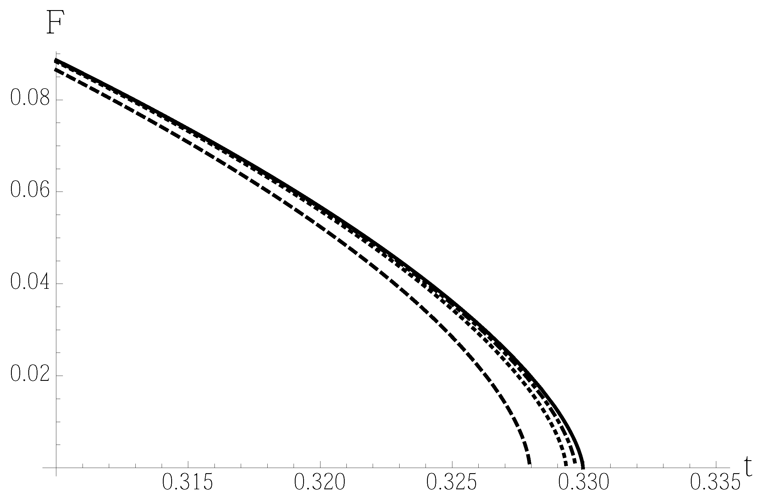
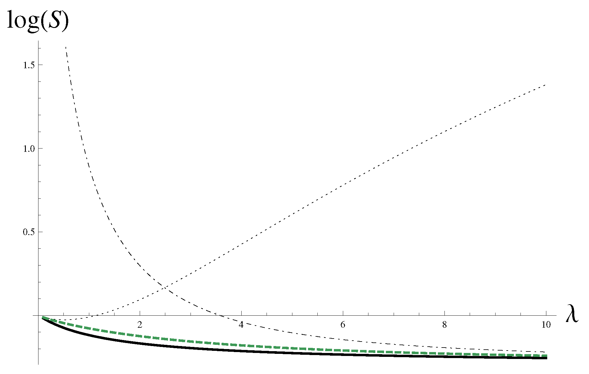
In Figure 8 the results from (76) are compared with the (77). They are in a good qualitative agreement, smoothly interpolating between the two regimes.

One can think that the problem is difficult, because of a wide crossover region between the two asymptotic regimes.

4.3.1. Schwinger Model. Interpolation

The Schwinger model [46,47] represents the Euclidean quantum electrodynamics interacting with a Dirac fermion field. It is defined on lattice in $(1+1)$ dimensions. It reflects on many properties, the confinement, chiral symmetry breaking, and charge shielding, with quantum chromodynamics. Most interesting, the structure of expansions for Schwinger model appears to remind closely the case of quartic anharmonic oscillator. Therefore, the same technique of construction approximants with counter-terms can be used.

Ground state. We test the technique of $DLog$ additive approximants first on the case previously explored in [38], and calculate the ground state of the model, given as a function of the dimensionless variable $x=m/g$. Here m stands for electron mass and g is the coupling parameter. It also has the dimension of mass. The energy is $E=M-2m$, corresponding to a vector boson of mass $M(x)$.

The expansion at small-x the expansion for the ground-state energy [48,49,50,51] is known as follows,

$$E(x)\simeq 0.5642-0.219x+0.1907x^2(x\to 0).$$

(78)

In the complementary, large-x limit [51,52,53,54], there is another truncated expansion

$$E(x)\simeq 0.6418x^{-1/3}-\frac{1}{\pi }{x}^{-1}-0.25208x^{-5/3}(x\to \infty ).$$

(79)

The self-similar root approximant $R_5^{*}(x)$ as defined as in (28), was applied to the interpolation between the two expansions [38]. Its detail expression can be also found in [38]. The accuracy of this approximant $R_5^{*}$ was compared in [38] to various results of calculations by other researchers. In particular, with the density matrix renormalization group, $E_{DMRG}$ [55], and fast moving frame estimates, $E_{FMFE}$ [56]. The ground state energy has also been calculated by using variational perturbation theory [57]. However the results were found to be rather cumbersome, and without advantage over other techniques.

With help of counter-terms, we proceed just like in the previous example of the quartic anharmonic oscillator, and set $\beta =\frac{1}{3}$ and $\gamma =\frac{1}{3}$. Then, with

$${\alpha }_1=0,x_0=-3{\alpha }_3,$$

the $DLog$-additive approximant reads in general form as follows,

$$\begin{array}{c}\frac{E_3^{*}(x)}{E_3^{*}(0)}=\frac{\exp \left(\frac{3}{2}{\alpha }_2\left(\frac{1}{{x_0}^{2/3}}-\frac{1}{{(x+x_0)}^{2/3}}\right)+{\alpha }_3\left(\frac{1}{x_0}-\frac{1}{x+f_0}\right)\right)}{\sqrt[3]{\frac{x}{x_0}+1}},\hfill \end{array}$$

(80)

and, after the parameters are computed, we obtain

$$E_3^{*}(x)=\frac{0.695641e^{\frac{0.261771}{x+0.785314}-\frac{0.461993}{{(x+0.785314)}^{2/3}}}}{\sqrt[3]{1.27338x+1}}.$$

(81)

Let us construct also “just” an additive approximant, which includes all terms from the two expansions for the grouns state energy. The additive approximant corresponds to the pair of complex-conjugated (C.C.) solutions, and the full solution is

$$E_{ad}^{*}(x)=\frac{(e_{ad}(x)+C.C.)}{2},$$

(82)

where

$$\begin{array}{c}{e}_{ad}(x)=\hfill \\ \frac{0.183245-0.0235908i}{{(1+(0.597191-0.241372i)x)}^{4/3}}-\frac{0.190092-0.0768311i}{1+(0.597191-0.241372i)x}-\frac{0.190092-0.0768311i}{{(1+(0.597191-0.241372i)x)}^2}+\hfill \\ \frac{0.549736-0.0707723i}{\sqrt[3]{1+(0.597191-0.241372i)x}}-\frac{0.097124-0.0723392i}{{(1+(0.597191-0.241372i)x)}^{5/3}}+\frac{0.60882-0.547284i}{{(1+(0.597191-0.241372i)x)}^{7/3}}\hfill \\ -\frac{0.300293-0.415646i}{{(1+(0.597191-0.241372i)x)}^{8/3}}.\hfill \end{array}$$

(83)

The accuracy of the approximant $E_{ad}^{*}$ can be compared to various results. We present such comparison in

Table 1. Ground-state energy (vector state) of Schwinger model, dependent on the nondimensional parameter x. Different approximations are compared, such as Density matrix renormalization group, $E_{DMRG}$; $DLog$-additive approximants, $E_{DLog}$; fast moving frame estimates, $E_{FMFE}$; the self-similar additive approximant $E_{ad}^{*}$; and self-similar root approximant $R_5^{*}$ from [38].

x	${\mathit{E}}_{\mathit{DMRG}}$	${\mathit{E}}_{\mathit{DLog}}$	${\mathit{E}}_{\mathit{FMFE}}$	${\mathit{R}}_5^{*}$	${\mathit{E}}_{\mathit{ad}}^{*}$
0	0.56419	0.564	N.A	0.564	0.564
0.125	0.5395	0.540	0.528	0.54	0.539
0.25	0.51918	0.520	0.511	0.519	0.519
0.5	0.48747	0.49	0.489	0.487	0.487
1	0.4444	0.444	0.455	0.444	0.442
2	0.398	0.397	0.394	0.392	0.389
4	0.340	0.342	0.339	0.337	0.334
8	0.287	0.287	0.285	0.284	0.282
16	0.238	0.237	0.235	0.235	0.235
32	0.194	0.193	0.191	0.192	0.192

, the energy $E_{DLogA}$, found by means of the $DLog$-additive approximant (81). All results are close to each other, being practically the same in the range of computational errors. The Padé approximant $P_{5,6}(x^{1/3})$ was also constructed in [38], and it worked with the same accuracy as other techniques. Concrete results for the ground state energy obtained with such approximant, can be found in [38].

Excited state. Consider now the first excited state of the model, corresponding to a scalar boson. The small-x expansion for the energy of the excited “scalar” state, can be extracted from [48,49,50,51] is given as follows,

$$E(x)\simeq 1.1284+1.562x-13.512x^2.$$

(84)

In the large-x limit [51,52,53,54], there is a another, complementary expansion

$$E(x)\simeq \frac{1.4729}{\sqrt[3]{x}}-\frac{0.31831}{x}+\frac{0.10847}{x^{5/3}}.$$

(85)

The problem appears to be more more difficult than ground state problem, likely, because of a non-monotonous crossover region for small x. The root approximant even brings apparently wrong, complex results in this case. Although it works well for the ground state, even solving the most difficult extrapolation problem [30,38], allowing to calculate the critical index at infinity with good accuracy.

We can also try to apply the Padé technique. It was already found to work well for the ground state [38]. Thus, the following Padé approximant $P_{5,6}(x^{1/3})$, was constructed. We found that it to be as good as other much more sophisticated techniques. Namely,

$$\begin{array}{c}{P}_{5,6}(x^{1/3})=\frac{2.69758x^{2/3}+9.5477x^{4/3}+11.0482x^{5/3}+2.69338\sqrt[3]{x}+5.20904x+1.1284}{2.39062x^{2/3}+5.15717x^{4/3}+6.4818x^{5/3}+7.501x^2+2.3869\sqrt[3]{x}+3.23204x+1}.\hfill \end{array}$$

(86)

Let us consider the $DLog$ additive technique. With counter-term

$${\alpha }_1=0,$$

the simplest $DLog$-additive approximant reads

$$\begin{array}{c}\frac{E_2^{*}(x)}{E_2^{*}(0)}=\frac{\exp \left(\frac{3}{2}{\alpha }_2\left(\frac{1}{{x_0}^{2/3}}-\frac{1}{{(x+x_0)}^{2/3}}\right)+3{\alpha }_1\left(\frac{1}{\sqrt[3]{x_0}}-\frac{1}{\sqrt[3]{x+x_0}}\right)\right)}{\sqrt[3]{\frac{x}{x_0}+1}}.\hfill \end{array}$$

(87)

and, after some calculations, we obtain

$$E_2^{*}(x)=\frac{2.65355e^{-\frac{0.263456}{{(x+0.171017)}^{2/3}}}}{\sqrt[3]{5.84739x+1}}.$$

(88)

Let us construct also “just” an additive approximant, which includes all terms from the two expansions from the scalar state energy. The additive approximant corresponds to the pair of complex-conjugated (C.C.) solutions, and the full solution is

$$E_{ad}^{*}(x)=\frac{(e_{ad}(x)+C.C.)}{2},$$

(89)

where

$$\begin{array}{c}{e}_{ad}(x)=\hfill \\ \frac{1.95492-2.53467i}{{(1+(2.20007-1.69363i)x)}^{8/3}}-\frac{2.39372-2.5837i}{{(1+(2.20007-1.69363i)x)}^{7/3}}-\frac{0.700304-0.539099i}{{(1+(2.20007-1.69363i)x)}^2}+\hfill \\ \frac{0.273332-0.528414i}{{(1+(2.20007-1.69363i)x)}^{5/3}}+\frac{0.673618-0.149705i}{{(1+(2.20007-1.69363i)x)}^{4/3}}-\frac{0.700304-0.539099i}{1+(2.20007-1.69363i)x}+\hfill \\ \frac{2.02085-0.449114i}{\sqrt[3]{1+(2.20007-1.69363i)x}}.\hfill \end{array}$$

(90)

The quality of the approximant $E_{ad}^{*}$ can be compared to data obtained in other calculations. For instance with finite lattice estimates, $E_{FL}$, obtained in [51], and fast moving frame estimates, $E_{FMFE}$ obtained in [56]. The energy has also been calculated by using variational perturbation theory [57]. But the latter lead to some rather complicated formulas, and no advantage over other techniques. In

Table 2. The energy of scalar state, or of the first excited state of Schwinger model, dependent on the dimensionless parameter x, in different approximations: Finite lattice estimates, $E_{FLE}$; $DLog$-additive approximant, $E_{DLog}$; fast moving frame estimates, $E_{FMFE}$; the self-similar additive approximant $E_{ad}^{*}$; and the Padé approximant $P_{5,6}$.

x	${\mathit{E}}_{\mathit{FLE}}$	${\mathit{E}}_{\mathit{DLog}}$	${\mathit{E}}_{\mathit{FMFE}}$	${\mathit{E}}_{\mathit{ad}}^{*}$	${\mathit{P}}_{5,6}$
0	1.11	1.13	N.A	1.13	1.13
0.125	1.22	1.22	1.314	1.21	1.24
0.25	1.24	1.23	1.279	1.23	1.26
0.5	1.20	1.19	1.227	1.22	1.24
1	1.12	1.1	1.128	1.15	1.15
2	1.00	0.97	0.991	1.01	1.01
4	0.85	0.83	0. 837	0.85	0.85
8	0.68	0.69	0. 690	0.7	0.7
16	0.56	0.56	0.559	0.57	0.56
32	0.45	0.45	0.447	0.45	0.45

, we compare the different data with our result $E_{ad}^{*}$. Also, we present the energy $E_{DLog}$ found by means of the $DLog$-additive approximant (88). The ground state energy calculated from the Padé approximant (86), is brought up as well. All results appear to be fairly close to each other.

The $DLog$-additive approximants appear to be the most consistent among other self-similar approximations. They are able to adapt well to both cases of ground and excited states. They appear to be as good as the other very heavy numerical techniques, but have the advantage of being more transparent. Modified Padé approximants are also able to solve the interpolation problem for the ground and excited states energies. The technique based on root approximants allows though, to attack successfully the most hard problem of the critical index at infinity, based on information encoded in the very short series for small x [30,38].

4.3.2. Correlation Energy of One-Dimensional Electron Gas. Interpolation

Below we present an accurate expression for the one-dimensional electron gas correlation energy. The energy is conveniently given in a reduced nondimensional form $\epsilon (r_s)$, Here $r_s$ stands for Seitz radius. Let recapitulate the known expansions for the to available asymptotic cases [58].

At small $r_s$ (high-densities) the following expansion for for the correlation energy is known [58],

$$ϵ(r_s)\simeq C+0.00845r_s(r_s\to 0),$$

where

$$C=-\frac{{\pi }^2}{360}=-0.027416.$$

In the opposite situation, for the large $r_s$ (low-densities) [58], the following expansion is available,

$$ϵ(r_s)\simeq \frac{b_1}{r_s}+\frac{b_2}{r_s^{3/2}}(r_s\to \infty ),$$

with

$$b_1=-\left(\ln \sqrt{2\pi }-\frac{3}{4}\right)=-0.168939,b_2=0.359933.$$

In our notations, the value of indices $\beta =-1$, $\gamma =1/2$. There are no need for counter-terms, meaning that the general recursion can be applied without complications in the original variables. The $DLog$-additive approximant, with the two asymptotic cases included, is supposed to work for arbitrary $r_s$. It reads as follows

$${ϵ}_2^{*}(r_s)=-\frac{0.168939e^{\frac{0.532019}{r_s+1.58887}-\frac{2.13056}{\sqrt{r_s+1.58887}}}}{r_s+1.58887}.$$

(91)

The series available to us are very short. In order to be able to go to the higher-order approximant, we can fix some unknown parameter to some plausible value. The $DLog$-additive approximant, with the same asymptotic expansions, but with the fixed parameter $g_0=1$, could be constructed as well,

$${ϵ}_3^{*}(r_s)=-\frac{0.168939e^{\frac{0.189402}{r_s+1}+\frac{0.12273}{\left(r_s+1\right){}^{3/2}}-\frac{2.13056}{\sqrt{r_s+1}}}}{r_s+1}.$$

(92)

Comparing the results of the two $DLog$-additive approximants with the data from diffusion Monte Carlo calculations [58] in the interval $0<r_s<20$, we find that the maximal error of ${\epsilon }_3^{*}$ is just $0.55\%$, and of ${\epsilon }_2^{*}$ is only $1.6\%$. The Padé approximants are not giving consistent results, while given such short series. They generate the errors varying between $2\%$ and $10\%$. For instance, $P_{1/2}(\sqrt{r_s})$ has reasonable error of $2\%$. But another approximant, $P_{0/3}(\sqrt{r_s})$, brings the maximal error of $10\%$.

Previously, in [32], the problem was attacked with root approximants, but the maximal error of $8\%$ was found. There is a very significant improvement achieved by applying the $DLog$-additive approximants. It is highly advantageous that the approximants allow to avoid fitting, bearing in mind those cases where no exact or even approximate numerical data are available. Besides, only in such setting the value of available expansions and quality of various approximants can be evaluated.

5. Concluding Remarks

It is likely a pipe dream to find the same approximant to be the best for each and every realistic problem. Rather we believe into “strength in numbers”, when different approximants are viewed as a group dedicated to the problem solution. Based on the same asymptotic material, such as series coefficients, thresholds, critical indices, correction to scaling indices one can construct not only Padé but also post-Padé approximations. With various approximants (Padé, $Log$-Padé, $DLog$-Padé, factor, root, corrected Padé, additive, $DLog$-additive etc.) available it is much more probable that for each problem one can find an optimal different one, or even a combination of the few. New approximants are always welcome, even if they allow to solve only a single problem.

Subjectively, we hope that the idea of corrected approximants [6,7,8,29], is going to have the last word. It allows to combine the strength of a few methods together and proceed, in the space of approximations, with piece-wise construction of the approximation sequences. The corrected approximants also possess strength in numbers.

The approximants are relatively easy to compute based on the known series. And the problem is now centered around finding the best approximation scheme for each concrete problem. It is not less important to have in mind a concrete validation and testing schematics, akin to those developed in machine learning. For instance, one can construct several initial guesses based not on all $c_k$, threshold, indices, but only on a part of them, leaving the rest for validation. The best guess could be chosen as the best descriptor to the validation set. After validation all parameters can be incorporated into chosen best approximant, and tested. In the field of effective properties one can use a few numerical points for testing [7,8]. One can also try to combine several approximants into a single “super-approximant”, by using regression on approximants [7], which would involve asymptotic information as well data points. Yet different method of combining such information was developed in [59].

We remind about another possible application of the approximants. It is notoriously difficult to get hold on the coefficients $c_n$, especially in high orders. One can try plainly (naively?) to generate additional coefficients $c_n$ from the approximants, as first suggested by Feynman. Sometimes, even the order of magnitude or the sign can be of value.