Article

An Extended Shapley TODIM Approach Using Novel Exponential Fuzzy Divergence Measures for Multi-Criteria Service Quality in Vehicle Insurance Firms

by
Arunodaya Raj Mishra
1,
Pratibha Rani
2,
Abbas Mardani
3,4,*,
Reetu Kumari
5,
Edmundas Kazimieras Zavadskas
6 and
Dilip Kumar Sharma
5
1
Department of Mathematics, Govt College, Jaitwara 485221, MP, India
2
Department of Mathematics, NIT, Warangal 506004, Telangana, India
3
Informetrics Research Group, Ton Duc Thang University, Ho Chi Minh City 758307, Vietnam
4
Faculty of Business Administration, Ton Duc Thang University, Ho Chi Minh City 758307, Vietnam
5
Department of Mathematics, Jaypee University of Engineering & Technology, Guna 473226, MP, India
6
Institute of Sustainable Construction, Vilnius Gediminas Technical University, Sauletekio Ave. 11, LT-10223 Vilnius, Lithuania
*
Author to whom correspondence should be addressed.
Symmetry 2020, 12(9), 1452; https://doi.org/10.3390/sym12091452
Submission received: 9 June 2020 / Revised: 6 August 2020 / Accepted: 26 August 2020 / Published: 3 September 2020
(This article belongs to the Special Issue Uncertain Multi-Criteria Optimization Problems)

Abstract

:
Classification of the divergence measure for fuzzy sets (FSs) has been a successful approach since it has been utilized in several disciplines, e.g., image segmentation, pattern recognition, decision making, etc. The objective of the manuscript is to show the advantage of the combined methodology. A comparison clearly shows the usefulness of the proposed technique over the existing ones under the fuzzy environment. This study presents novel exponential-type divergence measures with some elegant features, which can be applied to FSs. Next, a TODIM (an acronym in Portuguese for Interactive Multicriteria Decision Making) approach derived from prospect theory, Shapley function, and divergence measure for multi-criteria decision-making (MCDM) is proposed. Besides, for the reason of evaluating the dominance degree of the option, and the weights of the criteria, proposed divergence measures are implemented. Evaluating and selecting the service quality is the most important issue in management; it has a direct influence on the way the manufacturer performs its tasks. Selecting the service quality can be thought of as a problem of MCDM involving numerous contradictory criteria (whether of a quantitative or qualitative nature) for the evaluation processes. In recent years, the service quality assessment is becoming increasingly complex and uncertain; as a result, some criteria assessment processes cannot be efficiently done by numerical assessments. In addition, decision experts (DEs) may not always show full rationality in different real-life situations that need decision making. Here, a real service quality evaluation problem is considered to discuss the efficacy of the developed methods. The algorithm (TODIM based on the Shapley function and divergence measures) has a unique procedure among MCDM approaches, which is demonstrated for the first time in this paper.

1. Introduction

Shannon entropy [1] and Kullback–Leibler (K-L) [2] divergences are two critical measures in the information theory. On account of their accomplishment, there are several efforts to extend these notions. In the literature, the author(s) have achieved various information measures. K-L [2] pioneered the concept of divergence, which measures the discrimination level among probability distributions. Later on, numerous researchers developed several generalized divergence measures and described their behaviors and applications [3,4]. A novel measure called the Jensen–Shannon (J-S) divergence, which was introduced by Lin [5], which has received interest from researchers and been effectively implemented in various constraints [6,7].
Analogous to the idea of probability doctrine, Zadeh [8] initiated the conception of fuzzy sets (FSs) to handle the ambiguity that arises in daily life problems. The concept of fuzzy entropy measures refers to the amount of fuzziness that arises due to the ambiguity of being or not being a member of the set. Based on Shannon entropy, De Luca and Termini [9] pioneered the axiomatic definition of fuzzy entropy. Pal and Pal [10] decisively investigated Shannon’s function to propose novel entropy based on the exponential function. Hooda [11] developed two generalized measures based on fuzzy entropy. Based on exponential function, Verma and Sharma [12] studied a new generalized parametric fuzzy entropy. Mishra et al. [13] established logarithmic-fuzzy entropy with the applications in pattern recognition and medical diagnosis. Aside from these articles, copious numbers of fuzzy entropy have been developed by numerous authors [14,15,16,17].
Moreover, Bhandari and Pal [18] established the notion of the measure of divergence for FSs, which describes the measure of discrimination between FSs. Next, the exponential divergence measure for FSs was introduced by Fan and Xie [19] and deliberated its properties. An automated leukocyte recognition application of the divergence measure for FSs was discussed by Ghosh et al. [6]. Mishra et al. [12,15] proposed a discrimination measure for FSs and applied these measures to medical and crop diagnosis. Rani et al. [20] studied unified fuzzy divergence measures with an application in the e-waste recycling selection problem. Arora and Dhiman [21] presented a novel measure of fuzzy directed divergence with an application in decision making. Divergence measures for FSs and their extensions have ample applications in various disciplines viz. pattern recognition, signal and image processing, medical diagnosis, and so on [22,23,24,25].
Multi-criteria decision making (MCDM) has been proven as an important research discipline of decision science and is currently broadly applied in business and management [26,27], engineering [20,28], economy [29,30], and so on. In real-life applications, it is quite a challenging issue to find the solution of MCDM problems. Over the last few decades, several new MCDM methods have been introduced. By increasing the difficulty and the extensive changes in today’s environment, the classical MCDM methods were not adequate to deal with the practical MCDM problems. Nowadays, various procedures have been developed to tackle the MCDM problems, viz. the technique for order of preference by similarity to ideal solution (TOPSIS) [31,32], weighted aggregated sum product assessment (WASPAS) [33,34], multi-attributive border approximation area comparison (MABAC) [35,36], Vlse Kriterijumska Optimizacija Kompromisno Resenje (VIKOR) [37,38], ELimination and Choice Expressing REality (ELECTRE) [39,40], Preference Ranking Organization METHod for Enrichment of Evaluations (PROMETHEE) [41,42], TODIM (which is the acronym in Portuguese language for Interactive MCDM) [43,44] and so on.
The prospect doctrine is a descriptive doctrine that can be implemented in the process of making decisions under risk [45]. An MCDM technique named TODIM was introduced by Gomes and Lima [46] initially. The base of this technique was the prospect theory, and it was used to explain the MCDM problem in cases where the psychological behaviors of decision experts (DEs) are considered. Next, TODIM has also been widely employed in a variety of fields with decision-making problems, e.g., portfolio allocation and selection [43], internet banking website quality [47], and sustainability perspective [48]. In another study, Gomes et al. [49] considered the fact that relationships amongst different criteria are sometimes interdependent; thus, they introduced a method integrating TODIM and Choquet integral for the purpose of handling the MCDM problems using criteria interactions. TODIM was expanded by Qin et al. [50] using the interval-valued type-2 fuzzy sets to solve the green supplier selection problem. Mishra and Rani [51] presented the interval-valued intuitionistic fuzzy TODIM procedure based on bi-parametric information measures to evaluate the plant location selection problem. On the other hand, Hesitant-TODIM was introduced by Fan et al. [52] to handle the hybrid MCDM problems using interval, crisp, and fuzzy numbers. Liu and Shen [53] suggested the Choquet-TODIM method within a linguistic intuitionistic fuzzy set environment. Further, Zhang et al. [54] studied the TODIM approach for IFSs to rank the products with online reviews. Though TODIM was capable of effectively solving the decision-making problems using crisp numbers, in a variety of conditions, crisp data is not sufficient for modeling the decision-making issues in real-life problems. Moreover, the fuzzy set and their extended forms have been found to be more effective in modeling human judgments. It has encouraged lots of scholars to design extended forms of TODIM as this method efficiently solves the MCDM problems in a variety of fuzzy settings.
As we recognize, any MCDM problem aims to deal with two major concerns: (1) The weights of criteria (and experts), and (2) aggregation operators. Many scholars have taken into account the divergence measure because of its effectiveness in the evaluation of uncertain information. In such conditions, this is generally applied to acquiring the criteria weights for MCDM in uncertain environments [55,56]. Nevertheless, experts’ weights, criteria, and aggregation operators for FSs are all on the basis of the assumption indicating the significance of experts and criteria are considered only in their additive weights. Although, in several practical MCDM problems, the independent features between the experts and the criteria are generally violated. Therefore, numerous researchers have studied the fuzzy measure [57], which is an efficient tool for modeling the interactions between elements that exist within a set. In the case of the additive measures, such measures only make the monotonicity instead of additively. They can be used in numerous fields, especially in decision making and game theory.
Motivated by the above-mentioned works, the present paper proposes the new Jensen–Shannon exponential divergence (JSED) measures are applied to FSs and discusses some elegant properties, which are useful in improving the usefulness of the proposed measure. Next, a fuzzy TODIM technique for MCDM is proposed. To extend the F-TODIM method, the concepts of the Shapley function and divergence measure are used. In the course of calculating the criteria weight and the proposed method’s dominance degree, some modifications are done when necessary. Such integration is able to result in more realistic criteria weights for decision-making as well as higher stability in the various weights of criteria. We make use of an instance of the service quality selection problem in a way to show more clearly the process and to demonstrate how the proposed method performs its defined tasks when faced with real-world decision-making problems. At the final step, the proposed F-TODIM method is compared with some currently used methods, aiming at illustrating the obtained results’ validity.
The arrangement of this article is provided in the given sections. The preliminaries and the divergence measure for FSs are provided in Section 2. Section 3 introduces the novel Jensen–Shannon exponential divergence measures for FSs. Section 4 provides the integrated TODIM approach based on the Shapley function and divergence measure. In Section 5, the application of service quality as a case study and comparative analysis is provided. The conclusion of this study is provided in Section 6.

2. Preliminaries

For the probability distribution, Q = ( q 1 , q 2 , ,   q n ) Δ n , Shannon’s entropy [1] is described by
H ( Q ) = i = 1 n q i log q i ,
Additionally, Renyi entropy [3] is given as
H R ( Q ) = 1 α 1 ln ( i = 1 n q i α ) ,   where   α > 0 ,     α 1 .
The exponential entropy was suggested by Pal and Pal [10] as another measure as expressed below:
H P a l ( Q ) = i = 1 n q i e ( 1 q i ) 1 .
According to Pal and Pal [10], from a certain perspective, the exponential entropy is better than Shannon’s entropy [1]. In the uniform distribution Q = ( 1 n , 1 n , , 1 n ) , the measure (3) is fixed as the upper-bound lim n H ( 1 n , 1 n , , 1 n )   = e 1 , which is not possible for (1).
Later on, Kullback and Leibler (K-L) [2] introduced a divergence measure among the probability distributions Q and S, given as:
C K L ( Q | | S ) = i = 1 n q i log q i s i , .
Its symmetric version, i.e., Jeffrey’s invariant, is given by
J ( Q | | S ) = C K L ( Q | | S ) + C K L ( S | | Q ) .
Renyi divergence is associated with entropy (2) by various settings as follows:
C R ( Q | | S ) = 1 α 1 ln ( i = 1 n q i α s i 1 α ) ,     α > 0 ,     α 1 .
Lin [5] proposed the Jensen–Shannon divergence measure between two probability distributions Q and S, given as
C J S ( Q | | S ) = H ( Q + S 2 ) H ( Q ) + H ( S ) 2 ,
which H ( . ) stands for the Shannon entropy expressed earlier in (1).
For simplicity, Jensen–Shannon divergence (7) can be demonstrated regarding the K-L divergence as follows:
C J K ( Q | | S ) = 1 2 [ C J S ( Q | | Q + S 2 ) + C J S ( S | | Q + S 2 ) ] .

2.1. Fuzzy Sets (FSs)

Definition 1. 
(Zadeh [8]). A fuzzy set P on finite discourse set V = { v 1 ,     v 2 ,     ,     v n } is given by:
P = { ( v i , μ P ( v i ) ) : μ P ( v i ) [ 0 , 1 ] ;   v i V } ,
where the function μ P ( v i ) ( 0 μ P ( v i ) 1 ) is the membership degree of v i to P in V.
For P   F S ( V ) , we utilize P c to find the complement of P , i.e., μ P c ( v i ) = 1 μ P ( v i ) ,     v i   V . For P ,   E     F S s ( V ) ,     P E is given as   μ P E ( v i ) = max { μ P ( v i ) ,   μ E ( v i ) } . P E is defined as   μ P E ( v i ) = min { μ P ( v i ) ,   μ E ( v i ) } and P   E iff μ P ( v i )   μ E ( v i ) .
De Luca and Termini [9], for the first time, presented the definition of entropy for FSs.
Definition 2. 
(De Luca and Termini [9]). A real-valued mapping H : F S ( V ) R + is called an entropy on FS(V) if H satisfies the axioms:
( A 1 ) .   H ( D ) = 0 ,         D P ( V )   =   Set   of   all   crisp   sets   in     V ; ( A 2 ) .   H ( [ 1 2 ] ) = max P F S ( V ) H ( P ) ; ( A 3 ) .   H ( P * ) H ( P ) , P * is   the   sharper   version   of   P ;   and ( A 4 ) .   H ( P ) = H ( P c ) ,       P F S ( V ) .
Analogous to (1), De Luca and Termini [9] pioneered the constructive measure as:
H D ( P ) = 1 n     i = 1 n [ μ P ( v i ) ln μ P ( v i ) + ( 1 μ P ( v i ) ) ln ( 1 μ P ( v i ) ) ] .
Pal and Pal [20] firstly introduced the exponential fuzzy entropy corresponding to (2), which is:
H P ( P ) = 1 n ( e 1 ) i = 1 n [ μ P ( v i ) e ( 1 μ P ( v i ) ) + ( 1 μ P ( v i ) ) e μ P ( v i ) 1 ] .  
Further, Mishra et al. [15] studied an exponential fuzzy entropy measure as:
H A ( P ) = 1 n e ( e 1 ) i = 1 n [ e μ P ( v i ) e μ P ( v i ) ( 1 μ P ( v i ) ) e ( 1 μ P ( v i ) ) ] .

2.2. Divergence Measure for FSs

Indeed, the divergence measure is employed for the purpose of measuring the discrimination information. Montes et al. [58] constructed the definition of F-divergence measure based on axioms.
Definition 3. 
(Montes et al. [58]). Let P ,   E F S s ( V ) , then J : F S s ( V ) × F S s ( V ) is an F-divergence measure if it fulfills the given postulates:
( P 1 ) .   J ( P ,   E )   =   J ( E ,   P ) ; ( P 2 ) .     J ( P ,   E ) =   0   iff   P = E ; ( P 3 ) .     J ( P   T ,   E     T ) J ( P ,   E ) ,     T   F S ( V ) ;   and ( P 4 ) .   J ( P   T ,   E     T )     J ( P ,   E ) ,   T     F S ( V ) .
The simplest divergence measure for FSs, as suggested by Bhandari and Pal [18], is given as:
C ( P | | E ) = i = 1 n [ μ P ( v i )   log   μ P ( v i ) μ E ( v i ) + ( 1 μ P ( v i ) ) log   ( 1 μ P ( v i ) ) ( 1 μ E ( v i ) ) ] .
Fan and Xie [19] founded a new measure for FSs as:
C F X ( P | | E ) = i = 1 n [ { 1 ( 1 μ P ( v i ) ) e ( μ P ( v i ) μ E ( v i ) ) + ( 1 μ P ( v i ) ) e ( μ E ( v i ) μ P ( v i ) ) } ] .
The distance measure depicts the difference between the two fuzzy sets. Fan and Xie [19] defined the distance measure for FSs as follows:
Definition 4. 
(Fan and Xie [19]). A real-valued function d : F S s ( V ) × F S s ( V ) [ 0 , 1 ] is a distance measure for FSs if d fulfills the given postulates:
( D 1 ) .   d ( P ,   E )   =   d ( E ,   P ) ;         P , E F S s ( V ) ; ( D 2 ) .   d ( P ,   P ) = 0 ,       P F S ( V )   ; ( D 3 ) .   d ( P ,   P c )   = 1 ,       P   F S ( V ) ;   and   ( D 4 ) .   P ,   E ,   T F S s ( V ) ,   if   P   E T ,   then   d ( P , T ) d ( P , E )     and     d ( P , T ) d ( E ,   T ) .

3. New Divergence Measure for FSs

Here, we proposed the Jensen–Shannon divergence measure for FSs corresponding to Shannon entropy concepts and Jensen’s inequality. A key feature of the Jensen–Shannon divergence is the fact that to each probability distribution, a different weight can be allocated. Such a characteristic has made it appropriate for studying the decision problems in cases in which weights can be prior probabilities. The majority of divergence measures have been created for two probability distributions. In the case of some particular applications, e.g., taxonomy studies in biology and genetics, one is needed for measuring the overall difference of more than two distributions. It is completely possible to generalize the Jensen–Shannon divergence in order to arrange such a measure for any finite number of distributions. In addition, it can be effectively applied to multiclass decision making.

Jensen–Shannon Exponential Divergence Measures for FSs

The idea of the Jensen–Shannon divergence promoted the authors to introduce an innovative divergence measure to describe the distinction between two fuzzy FSs and demonstrate various elegant properties.
Definition 5. 
Let P ,   E F S s ( V ) . Based on Mishra et al. [15], an exponential Jensen–Shannon divergence measure for P and E is described as follows:
C e ( P | | E ) = H A ( P + E 2 ) ( H A ( P ) + H A ( E ) 2 ) = 1 n e ( e 1 ) i = 1 n [ ( μ P ( v i ) + μ E ( v i ) 2 ) exp ( μ P ( v i ) + μ E ( v i ) 2 )     + ( 2 μ P ( v i ) μ E ( v i ) 2 ) exp ( 2 μ P ( v i ) μ E ( v i ) 2 ) 1 2 ( μ P ( v i ) exp ( μ P ( v i ) ) + ( 1 μ P ( v i ) ) exp ( 1 μ P ( v i ) )         + μ E ( v i ) exp ( μ E ( v i ) ) + ( 1 μ E ( v i ) ) + exp ( 1 μ E ( v i ) ) ) ] .
Next, to test the validity of measure (14), we established the given theorem.
Theorem 1. 
For P ,   E ,   T     F S s ( V ) , the measure (14) holds the following postulates:
( a )   C e ( P | |   E ) 0   and   0 C e ( P | |   E ) 1 , ( b )   C e ( P | |   E ) = 0   if   and   only   if   P = E , ( c )   C e ( P | |   E ) = C e ( E | | P ) , ( d )   C e ( P | | P c ) = 1 ,   if   and   only   if   P P ( V ) , ( e )   C e ( P | | E ) = C e ( P c | | E c )   and   C e ( P | | E c ) = C e ( P c | | E ) , and ( f )   C e ( P | | E ) C e ( P | | T )   and   C e ( E | | T ) C e ( P | | T ) ,   for   P E T .
Proof. 
The proof of the theorem is given in Appendix A.1. □
Proposition 1. 
If E = P c , then the relation between C e ( P | | E ) and H A ( P ) :
H A ( P ) = 1 C e ( P | | E ) ,
where H A ( P ) is entropy for FSs(V).
Proof. 
The proof is given in Appendix A.2. □
Corollary 1. 
The measure C e ( P | | E ) is the distance measure on FSs(V).
Proof. 
From Theorem 1, C e ( P | | E ) fulfills all the essential postulates of the distance measure (Definition 6). Hence, C e ( P | | E ) is also a distance measure for FSs(V). □
Proposition 2. 
For all P ,   E F S s ( V ) ,
( a )   C e ( P | | P E ) = C e ( E | | P E ) , ( b )   C e ( P | | P E ) = C e ( E | | P E ) , ( c )   C e ( P E | | P E ) = C e ( P | | E ) , ( d )   C e ( P | | P E ) + C e ( P | | P E ) = C e ( P | | E ) ,   and ( e )   C e ( E | | P E ) + C e ( E | | P E ) = C e ( P | | E ) .
Proof. 
The proof is given in Appendix A.3. □
Next, Jain and Chhabra [59] develop the exponential divergence measure for FSs as follows:
C J C ( P ,   E ) = i = 1 n [ ( μ P ( v i ) μ E ( v i ) ) exp ( μ P ( v i ) μ E ( v i ) ) + ( μ E ( v i ) μ P ( v i ) ) exp ( 1 μ P ( v i ) 1 μ E ( v i ) ) ] .
Moreover, the symmetric divergence measure for FSs P and E is defined as:
C J C ( P | | E ) = i = 1 n [ ( μ p ( v i ) μ E ( v i ) ) { exp ( μ P ( v i ) μ E ( v i ) ) exp ( 1 μ P ( v i ) 1 μ E ( v i ) ) } ] .
There is not any need for non-negativity of the divergence in the previous axioms, but this is too insignificant to deduce it from Definition 2. Now, suppose μ E ( v i ) = 0 . Then, from (16) and (17), C J C ( P , E ) and C J C ( P | | E ) are undefined. To overcome this drawback, based on Jain and Chhabra [59], we develop a new modified exponential divergence measure for FSs as follows:
C 2 ( P | | E ) = 1 n ( exp ( 2 ) 1 ) i = 1 n [ ( μ P ( v i ) μ E ( v i ) ) exp ( μ P ( v i ) 1 2 ( μ P ( v i ) + μ E ( v i ) ) ) + ( μ E ( v i ) μ P ( v i ) ) exp ( 1 μ P ( v i ) 1 1 2 ( μ P ( v i ) + μ E ( v i ) ) ) ] .
Theorem 2. 
For all P , E ,   T F S s ( V ) , then the measure C 2 ( P | | E ) given by (18) holds the postulates given in Theorem 1.
Proof. 
Proof is the same as Theorem 1. □
Corollary 2. 
The mapping C 2 ( P | | E ) is the distance measure on FSs(V).
Proof. 
Proof is obvious. □

4. An Integrated TODIM Approach Using the Shapley Function and Divergence Measure

Here, the conventional TODIM method is extended according to the Shapley function and divergence measure under the FSs context.

4.1. Shapley Function

Historically, the concept of fuzzy measures was pioneered in 1974 by Sugeno [60], and it would become well-known as an efficient instrument for modeling the interaction phenomena and addressing the decision-making problems [61,62,63].
Definition 6. 
(Sugeno [60]). A mapping g : P ( V ) [ 0 ,   1 ] is recognized as a fuzzy measure (F-measure) on V = { v j :   j = 1   ( 1 )   n } , if it fulfills the given requirements:
( a )   g ( ) = 0 ,     g ( V ) = 1 ;   and ( b )   If   E F ,   then   g ( E ) g ( F ) ,       E ,   F V .
In MCDM procedures, g ( E ) can be represented by the consequence of criteria E. As a result, the typical weights upon the criteria are taken in an independent way, and also the weights upon any set of criteria are suggested. Subsequently, the interactions that exist amongst the criteria are characterized. If v j E g ( v j ) for any E P ( V ) , then the fuzzy measure g deteriorates as an additive measure.
Lots of studies have been carried out onthe Shapley function [64] as a key interaction index; it is articulated as follows:
ϕ j ( g ,     V ) = K V \ v j ( n k 1 ) !     k ! n ! [ g ( K { v j } ) g ( K ) ] ,       v j   V ,
where g is a F-measure on V.
Here, the set K is characterized as an association that is generated by the game theory players, and it is perceived as a criterion set in the MCDM topic. The Shapley value ϕ j assumes as a category the mean value of the input of the object v j in any associations K \ v j . Furthermore, ϕ j ( g ,   V ) = g ( v j ) , when there is no connection.
Property 1. 
If g : P ( V ) [ 0 ,   1 ] is an F-measure, then ϕ j ( g ,   V ) 0 ,       v j V ;     j =   1 ( 1 ) n .
Property 2. 
If g : P ( V ) [ 0 ,   1 ] is an F-measure, then j = 1 n ϕ j ( g ,   V ) = g ( V ) = 1 .
Thus, { ϕ i ( g ,   V ) :     i = 1 ( 1 ) n } is a weight value.

4.2. Models for Criteria Weight Based on the Optimal Additive Measure

The entropy of criteria values needs to be taken into account; then, in case the information in regard with the criteria weights is partly unknown, or if it is completely unidentified, the amount of entropy for criteria v i ( i = 1 ( 1 ) n ) is suggested as i = 1 n H ( ε i j ) , where ε i j signifies a fuzzy number (FNs) of the option Si concerning the criterion Ej. In accordance with the entropy rule, if the entropy of an object is small, it would deliver valued information to the DEs. As a result, the criterion needs to be consigned with a greater weight; unless, the criterion would be considered insignificant by most DEs. In addition, this criterion needs to be estimated as a smaller weight. Hence, the optimal F-measure will form a greater inclusive value for each alternative that is preferable.
Remember that in this system, no option is inferior, and information associated to the criteria weights is completely unknown; therefore, to have the best fuzzy measure, the linear programming model on criteria E is formed by:
min j = 1 n i = 1 m H α ( ε i j ) ϕ j ( g ,   E ) s . t . { g ( ) = 0 ,     g ( E ) = 1 ,     g ( K ) g ( L )             K ,     L E ,   K L ,
while information associated with the criteria weights are partially known, then, for the optimal F-measure, the linear programming model on criteria E is assembled:
min j = 1 n i = 1 m H α ( ε i j )   ϕ j ( g ,   E ) s . t . { g ( ) = 0 ,     g ( E ) = 1 ,     g ( E j ) T j ,       j = 1 ( 1 ) n , g ( K ) g ( L )     K ,   L E ,   K L ,
where ϕ j ( g ,   E ) is the Shapley degree of criteria E j ( j = 1 ( 1 ) n ) and T j = [ t j ,   t j + ] is its range.

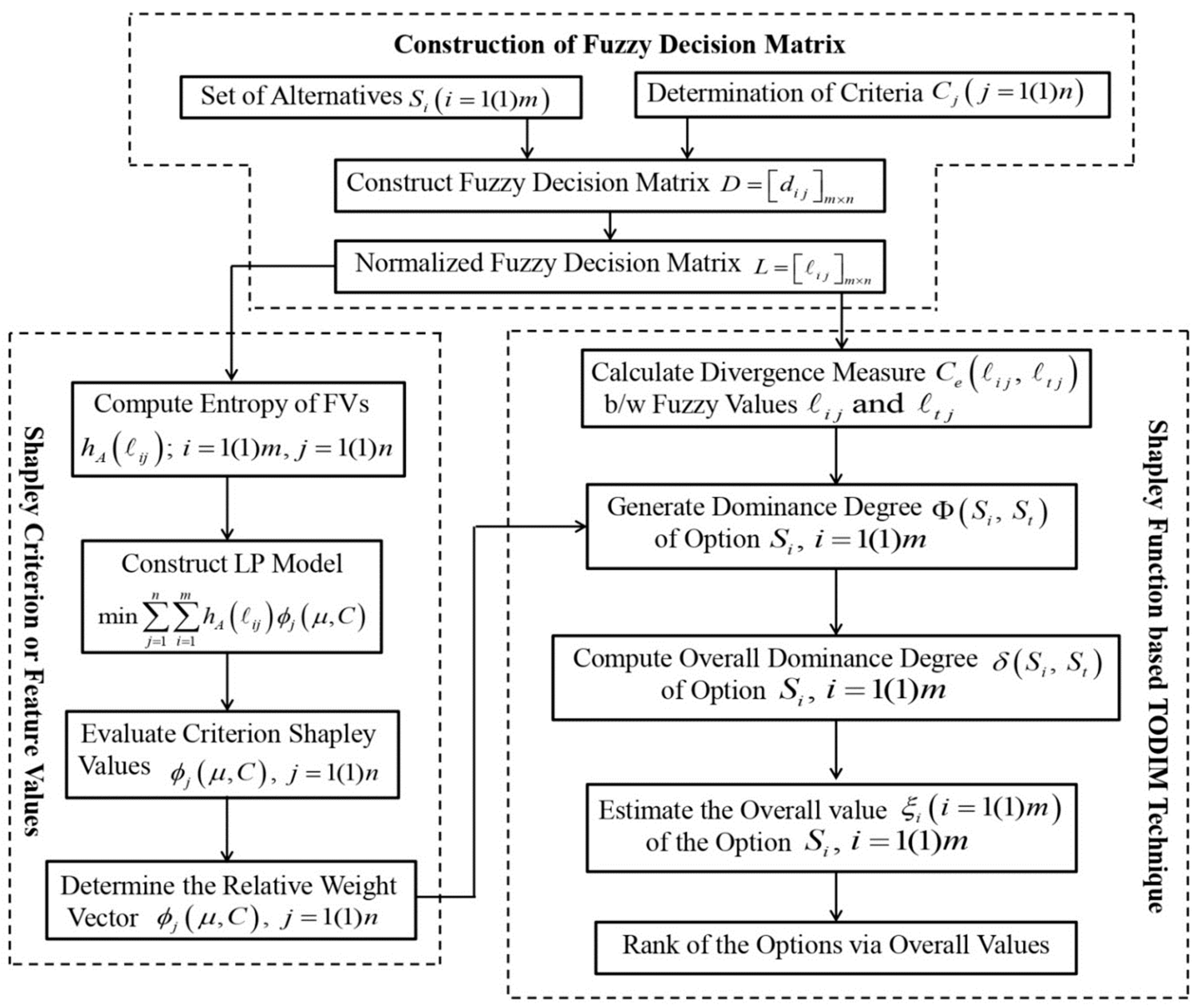
4.3. Shapley Function-Based TODIM Technique for MCDM

TODIM [46] was initially introduced to carefully take into consideration the psychological behaviors of decision making (DM). This tool is also capable of handling the MCDM problems efficiently. According to the prospect theory, through the use of this approach, the user can determine the dominance of each option over the different ones by creating a multi-values function [65].
Let S i ( i = 1 ( 1 ) m ) be the options on criteria E j ( j = 1 ( 1 ) n ) , then the procedure for the Shapley function-based TODIM technique is as follows (see Figure 1).
Step I: Construct a decision matrix D = ( d i j ) m × n , in which d i j presents an assessment value of an option Si concerning the criterion Ej. Initially, the information should be normalized. A larger value shows a higher quality assessment of benefit criteria, but the same condition reveals the poorer quality performance of a cost criterion. As a result, for the purpose of guaranteeing all criteria to be with complete compatibility, the cost criteria were transformed into benefit one using the formula below: i j = { d i j ,             for     benefit     criterion     E j ( d i j ) c ,     for     cos t     criterion     E j , where ( d i j ) c denotes the complement of d i j , through this procedure, and it is possible to attain the normalized fuzzy decision matrix L = ( i j ) m × n .
Step II: For a better judgment, we need to identify the significance of the judgment of each DE. Therefore, each criterion weight needs to be determined. If the characteristics among the criteria are interdependent, the weight vector of the criteria is calculated in forms of Shapley values. Employ (19), and model (20) and (21) with respect to (11), to find the criteria weight.
Step III: Calculate the criteria’s relative weight vector using the formula φ j r ( g ,     V )   = φ j ( g ,   V ) φ r ( g ,   V ) , where φ r ( g ,   V ) =   max { φ j ( g ,   V ) } and φ j ( g ,   V ) is the criteria weight Ej.
Step IV: Determine the degree of dominance of an option S i over each option S t by:
Φ j ( S i ,   S t )   =   {         φ j r ( g ,   V )     C e ( i j ,   t j ) j   =   1 n φ j r ( g ,   V )   ,                                     i f   i j >   t j                         0 ,                                                                                   i f   i j =   t j   1 θ   j   =   1 n φ j r ( g ,   V )   C e ( i j ,   t j ) φ j r ( g ,   V )   ,           i f   i j <     t j ,
measure between the fuzzy numbers i j and t j by using formula (14), and factor θ denotes the attenuation degree of the losses. If i j >   t j , then Φ j ( S i ,   S t ) characterizes again and if i j <     t j , then Φ j ( S i ,   S t ) denotes a loss.
Step V: Evaluate the overall dominance value of an option S i over each option S t by:
δ ( S i ,   S t )   =   j   =   1 n Φ j ( S i ,   S t ) ,     ( i ,   t =   1 ,   2 , , m ) .
Step VI: Determine the overall value of each option Si using the expression:
ξ i = t   =   1 m δ ( S i ,   S t ) min i { j   =   1 n δ ( S i ,   S t ) } max i { j   =   1 n δ ( S i ,   S t ) } min i { j   =   1 n δ ( S i ,   S t ) } ,     i =   1 ,   2 ,   , m .
Step VII: Determine the rank of options based on the overall values.

5. Case Study of the Proposed Method

Typically, in the evaluating process of the service quality, a set of m options S i   ( i = 1 , 2 , , m ) is involved. In this case, options refer to vehicle insurance firms. The service quality of these firms delivered to their customers is evaluated by the customers, which is denoted by a set of n criteria E j     ( j = 1 , 2 , , n ) . Toloie et al. [66] suggested a modified survey questionnaire for the purpose of estimating the customer-perceived quality of services. Four vehicle insurance firms that were chosen for this study are Oriental Insurance (S1), National Insurance (S2), Bajaj Insurance (S3), and New India Insurance (S4). The questionnaires indices contain four evaluation criteria, i.e., confidence (E1), responsiveness (E2), reliability (E3), and tangibles (E4).
Step I: Through the integration of the preference value results obtained from the four above-noted firms based on four evaluation criteria, the decision matrix of options is attained, as presented in Table 1. The importance of criteria is given by [ 0.15 ,   0.4 ] ,   [ 0.25 ,   0.5 ] ,   [ 0.25 ,   0.6 ] , and [ 0.2 ,   0.3 ] .
Step II: By using (11), the entropy measure of the option S i   ( i   = 1 ,   , 4 ) , considering the criteria E j ;   j   =   1 ( 1 ) 4 , is listed in Table 2.
From Table 2, the next LP-model is constructed:
min   [ 0.0160   { μ ( E 1 ) μ ( E 2 ,   E 3 ,   E 4 ) }   + 0.0044   { μ ( E 2 ) μ ( E 1 ,   E 3 ,   E 4 ) } +   0.0121   { μ ( E 3 ) μ ( E 1 ,   E 2 , E 4 ) }     0.0005   { μ ( E 4 ) μ ( E 1 ,   E 2 ,   E 3 ) } 0.0058   { μ ( E 1 ,   E 2 ) μ ( E 3 ,   E 4 ) } 0.0019   { μ ( E 1 ,   E 3 ) μ ( E 2 ,   E 4 ) } 0.0083   { μ ( E 1 ,   E 4 ) μ ( E 2 ,   E 3 ) } +   2.0578 ]
such that
{ μ ( E 1 )   μ ( E 1 ,   E 2 ) ,   μ ( E 1 ) μ ( E 1 ,   E 3 ) ,   μ ( E 1 ) μ ( E 1 ,   E 4 ) ,   μ ( E 2 )   μ ( E 1 ,   E 2 ) ,   μ ( E 2 ) μ ( E 2 ,   E 3 ) ,     μ ( E 2 ) μ ( E 2 ,   E 4 ) , μ ( E 3 )     μ ( E 1 ,   E 3 ) ,   μ ( E 3 )     μ ( E 2 ,   E 3 ) , μ ( E 3 )     μ ( E 3 ,   E 4 ) ,     μ ( E 4 )     μ ( E 1 ,   E 4 ) ,   μ ( E 4 )     μ ( E 2 ,   E 4 ) ,   μ ( E 4 )     μ ( E 3 ,   E 4 ) ,     μ ( E 1 ,   E 2 )     μ ( E 1 ,   E 2 ,   E 3 ) ,   μ ( E 1 ,   E 3 )     μ ( E 1 ,   E 2 ,   E 3 ) ,   μ ( E 2 ,   E 3 )     μ ( E 1 ,   E 2 ,   E 3 ) , μ ( E 1 ,   E 4 )     μ ( E 1 ,   E 2 ,   E 4 ) ,   μ ( E 2 ,   E 4 )     μ ( E 1 ,   E 2 ,   E 4 ) , μ ( E 1 ,   E 2 )     μ ( E 1 ,   E 2 ,   E 4 ) ,     μ ( E 1 ,   E 3 )     μ ( E 1 ,   E 3 ,   E 4 ) ,   μ ( E 1 ,   E 4 )     μ ( E 1 ,   E 3 ,   E 4 ) ,   μ ( E 3 ,   E 4 )     μ ( E 1 ,   E 3 ,   E 4 ) , μ ( E 1 ,   E 2 ,   E 3 )     μ ( E 2 ,   E 3 ,   E 4 ) ,   μ ( E 3 ,   E 4 )     μ ( E 2 ,   E 3 ,   E 4 ) , μ ( E 2 ,   E 4 )     μ ( E 2 ,   E 3 ,   E 4 ) , μ ( E 1 ,   E 2 ,   E 3 )     1 ,   μ ( E 1 ,   E 3 ,   E 4 )     1 ,   μ ( E 1 ,   E 2 ,   E 4 )     1 ,   μ ( E 2 ,   E 3 ,   E 4 )     1 ,   μ ( E 1 )     [ 0.15 ,   0.4 ] ,   μ ( E 2 )     [ 0.25 ,   0.5 ] ,   μ ( E 3 )     [ 0.25 ,   0.6 ] ,   μ ( E 4 )     [ 0.2 ,   0.3 ]   .
Solving (25) using MATHEMATICA, the F-measures on the criteria Ej are as follows:
μ ( E 1 )   =   0.4 ,   μ ( E 2 ) =   0.25 = μ ( E 3 ) ,   μ ( E 4 )   = 0.25 ,   μ ( E 2 ,   E 3 ) = 0.25 =   μ ( E 2 ,   E 4 ) = μ ( E 3 ,   E 4 )   , μ ( E 1 ,   E 2 ,   E 3 )   = 1 =   μ ( E 1 ,   E 2 ,   E 4 )   =   μ ( E 1 ,   E 3 ,   E 4 ) ,   μ ( E 1 ,   E 2 )   = 1 =   μ ( E 1 ,   E 3 ) =   μ ( E 1 ,   E 4 ) , μ ( E 2 ,   E 3 ,   E 4 )   =   0.25 ,   μ ( E 1 ,   E 2 ,   E 3 ,   E 4 )   = 1 .
The calculated Shapley values are
φ E 1 H A ( g ,   V ) =   0.6625 ,     φ E 2 H A ( g ,   V ) =   0.1125 ,     φ E 3 H A ( g ,   V )   =   0.1125 ,     φ E 4 H A ( g ,   V ) =   0.1125   .  
As a result, the Shapley degrees of the criteria are attained as follows:
W =   ( φ E 1 H A ( g ,   V )   ,   φ E 2 H A ( g ,   V )   ,   φ E 3 H A ( g ,   V ) ,   φ E 4 H A ( g ,   V ) ) T = ( 0.6625 ,   0.1125 ,   0.1125 ,   0.1125 ) T .
Step III: The relative weights of the given criteria E j ;   j   = 1 ( 1 ) 4 are φ 1 r ( g ,   V )   = 1 ,   φ 2 r ( g ,   V )     = 0.1698 ,   φ 3 r ( g ,   V )     = 0.1698   , and φ 4 r ( g ,   V )     = 0.1698 .
Step IV: The dominance degree matrices of the options over the criteria E j ;   j   = 1 ( 1 ) 4 are as follows:
Φ 1   =   [ 0 0.1966 0.2398 0.2928 0.1302 0 0.0426 0.0967 0.1589 0.0282 0 0.0521 0.1940 0.0641 0.0345 0 ] , Φ 2   =   [ 0 0.0225 0.0769 0.0225 0.2000 0 0.0543 0.0052 0.6838 0.4826 0 0.4808 0.2000 0.0459 0.0541 0 ] , Φ 3   =   [ 0 0.4971 0.0049 0.0258 0.0559 0 0.0379 0.0578 0.0439 0.3373 0 0.0201 0.2290 0.5138 0.1789 0 ] , Φ 4   =   [ 0 0.5147 0.1155 0.4571 0.0579 0 0.0439 0.0084 0.0130 0.3899 0 0.3307 0.0514 0.0744 0.0372 0 ] .
Step V: The total dominance degree matrix of option S i over each option S t is evaluated as:
δ   =   [ 0 1.1859 0.2735 0.7016 0.0440 0 0.0935 0.0253 0.5558 1.1816 0 0.8435 0.1836 0.5700 0.0531 0 ] .
Step VI: Now, the calculated overall values are as follows:
ξ 1   =   0.1559 ,   ξ 2   =   1.0000 ,   ξ 3   =   0.0000 ,   ξ 4   =   0.6588 .
Step VII: Finally, the ranking of the alternatives is S 2     S 4     S 1     S 3 and thus, S 2 is the optimal choice.
It is mentioned that any conflict does not exist in the preference ordering of all the options via the proposed technique and Mishra [67] technique. There is only one distinction between the proposed, and Mishra et al.’s [68] technique is obtained in deciding the preference ordering of S1 and S4. Additionally, the ranking obtained via the proposed technique is totally different from the Krohling, and de Souza [69] and Fan et al. [52] techniques (see Table 3).

Comparative Analysis

Here, the comparison of methods is based on a set of characteristics to adequately deal with the problem of service selection as follows:
In Mishra [67], the TOPSIS method is presented to find the solution of the MCDM problem, which is not capable of demonstrating the DMs behaviors. While, in this study, the TODIM approach is used to find the accurate solution of the MCDM problem, which assumes the psychological attitudes on DEs under risk. In the proposed method, we applied a fuzzy measure-based Shapley function to calculate the weight vector, which relaxes the additive condition of the conventional measure to the monotonicity condition. The fuzzy measure is a very important tool to deal with the criteria interaction. In Mishra [67], the entropy approach is used for the determination of the criteria weight. In the entropy method, in case the entropy value of each of the existing criteria is smaller than that of the available alternatives, a greater weight needs to be allocated to the criterion; otherwise, the criterion needs to be evaluated with a smaller weight. The authors in Mishra et al. [68] attempted to find out the criteria weight vector using the ordered weighted operator. The aggregation arguments need to be ordered before being aggregated. In Fan et al. [52] and Krohling, and de Souza [69], the criteria weights are assumed by the DMs.
The proposed method makes a ranking system for the available options through the measurement of their values of loss and gain and provides a significant total value for each one of the options; whereas, in Mishra [36], the authors made use of the positive-ideal value (PIV) and negative-ideal value (NIV) as benchmarks, which may be unrealistic to be the attained practically. By calculating the overall values in the developed method, we found that the related performance of all options with respect to each other on the considered factors or criteria. On the other hand, the score function applied in Mishra et al. [68] does not consider the related performance of all options with regards to each other, thereby it loses some valuable information, which can be helpful in the determination of the alternatives’ rank. The developed method is applied to deal with both independent and interdependent sets of criteria. However, the approach developed in Fan et al. [52], Krohling and de Souza [69], Mishra et al. [68], and Mishra [67] is only applicable for an independent set of criteria. Thus, the developed approach is more effective and reliable than the existing ones.

6. Conclusions

TODIM was found to be efficient in the solution of the MCDM-related problems, especially in the conditions in which the behaviors of DMs are taken into consideration, although the approach fails to solve the MCDM procedures directly under the FSs. In the present study, we proposed new exponential-type divergence measures for FSs and demonstrated many elegant properties, which were found to be capable of enhancing the usefulness of the proposed measure. Next, a TODIM method for MCDM based on the prospect theory, Shapley function, and divergence measure was developed. Models for optimal F-measures on the criteria or experts set via the Shapley function are, respectively, constructed, where the weights information of the DEs and the criteria are partly or fully unknown. A real service quality selection problem was used to express the effectiveness of the considered approach. The comparative discussion was demonstrated to exemplify the advantages of the proposed technique over the existing techniques for MCDM problems under the fuzzy environment.
Meanwhile, we will integrate the TODIM approach with various conventional MCDM methods like Preference PROMETHEE, stepwise weight assessment ratio analysis (SWARA), and analytic hierarchy process (AHP) methods. The method introduced in this study has the potential to be generalized to the MCDM procedures with interdependent criteria on PFSs and HFSs; in addition, it can be applied to comparable MCDM problems, e.g., risk investment, healthcare waste management, and performance evaluation.

Author Contributions

Conceptualization, A.R.M. and P.R.; methodology, A.R.M. and P.R.; software, P.R. and R.K.; validation, A.M., A.R.M. and P.R.; formal analysis, A.R.M. and D.K.S.; investigation, A.M.; resources, D.K.S.; data curation, R.K.; writing—original draft preparation, A.R.M. and P.R.; writing—review and editing, A.M. and E.K.Z.; visualization, A.M.; supervision, E.K.Z.; All authors have read and agreed to the published version of the manuscript.

Funding

This research received no external funding.

Conflicts of Interest

The authors declare no conflict of interest.

Appendix A

Appendix A.1. Proof of Theorem 1

(a) & (b). Let:
C e ( P | | E ) = 1 n i = 1 n ξ ( μ P ( v i ) , μ E ( v i ) ) ,       v i     V , where   ξ ( μ P ( v i ) , μ E ( v i ) ) = 1 e ( e 1 ) [ ( μ P ( v i ) + μ E ( v i ) 2 ) exp ( μ P ( v i ) + μ E ( v i ) 2 ) + ( 2 μ P ( v i ) μ E ( v i ) 2 ) exp ( 2 μ P ( v i ) μ E ( v i ) 2 ) 1 2 ( μ P ( v i ) exp ( μ P ( v i ) ) + ( 1 μ P ( v i ) ) exp ( 1 μ P ( v i ) ) + μ E ( v i ) exp ( μ E ( v i ) ) + ( 1 μ E ( v i ) ) exp ( 1 μ E ( v i ) ) ) ] .
Since f = v i exp ( v i ) and 0 v i 1 , then f = ( 1 +   v i ) exp ( v i ) 0 and f = ( 2 +   v i ) exp ( v i ) > 0 , ; thus, f is a concave up mapping of v i and C e ( P | | E ) is a convex function. Therefore, ξ ( μ P ( v i ) , μ E ( v i ) ) increases as P E γ increases such that P E γ = | μ P μ E | , and attains its maximum at P = { 1 } ,     E = { 0 } ( or   P = { 0 } , E = { 1 } ) , i.e., P ,   E P ( V ) and attains its minimum P = E . Hence, 0 C e ( P | | E ) 1 and C e ( P | | E ) = 0 if P = E .
(c). It is evident from (14), we obtain:
C e ( P | | E ) = C e ( E | | P ) .
(d) & (e). Both are obvious; therefore, the proofs are omitted.
(f). Let P E T , i.e., μ P μ E μ T , then E T γ P   E γ and P E γ P   T γ . Therefore, C e ( P | | E ) C e ( P | | T ) and C e ( E | | T ) C e ( P | | T ) , for P E T .

Appendix A.2. Proof of Proposition 1

C e ( P | | P c ) = 1 n e ( e 1 )   × i = 1 n [ ( μ P ( v i ) + μ P c ( v i ) 2 ) exp ( μ P ( v i ) + μ P c ( v i ) 2 ) ( 2 μ P ( v i ) μ P c ( v i ) 2 ) exp ( 2 μ P ( v i ) μ P c ( v i ) 2 ) 1 2 ( μ P ( v i ) exp ( μ P ( v i ) ) + ( 1 μ P ( v i ) ) exp ( 1 μ P ( v i ) ) + μ P c ( v i ) exp ( μ P c ( v i ) ) + ( 1 μ P c ( v i ) ) exp ( 1 μ P c ( v i ) ) ) ] .
It implies:
1 C e ( P | | P c ) = 1 + 1 n e ( e 1 ) × i = 1 n [ e ( μ P ( v i ) exp ( μ P ( v i ) ) + ( 1 μ P ( v i ) ) exp ( 1 μ P ( v i ) ) ) ] = 1 n e ( e 1 ) i = 1 n [ e μ P ( v i ) e μ P ( v i ) ( 1 μ P ( v i ) ) e ( 1 μ P ( v i ) ) ] = H A ( P ) .
Hence:
1 C e ( P | | E ) = H A ( P ) .

Appendix A.3. Proof of Proposition 2

To prove the (i)–(v), we consider that the finite discourse set V is divided into two disjoint sets V1 and V2 as:
V 1 = { v i | v i V ,   μ P ( v i ) μ E ( v i ) }       and       V 2 = { v i | v i V ,   μ P ( v i ) < μ E ( v i ) } .
(a). From (14), we have:
C e ( P | | P E ) = 1 n e ( e 1 )   i = 1 n [ ( μ P ( v i ) + μ P E ( v i ) 2 ) exp ( μ P ( v i ) + μ P E ( v i ) 2 ) ( 2 μ P ( v i ) μ P E ( v i ) 2 ) exp ( 2 μ P ( v i ) μ P E ( v i ) 2 ) 1 2 ( μ P ( v i ) exp ( μ P ( v i ) ) + ( 1 μ P ( v i ) ) exp ( 1 μ P ( v i ) ) + μ P E ( v i ) exp ( μ P E ( v i ) ) + ( 1 μ P E ( v i ) ) exp ( 1 μ P E ( v i ) ) ) ] = 1 n e ( e 1 )   [ v i V 1 { ( μ P ( v i ) + μ P ( v i ) 2 ) exp ( μ P ( v i ) + μ P ( v i ) 2 ) ( 2 μ P ( v i ) μ P ( v i ) 2 ) exp ( 2 μ P ( v i ) μ P ( v i ) 2 ) 1 2 ( μ P ( v i ) exp ( μ P ( v i ) ) + ( 1 μ P ( v i ) ) exp ( 1 μ P ( v i ) ) + μ P ( v i ) exp ( μ P ( v i ) ) + ( 1 μ P ( v i ) ) exp ( 1 μ P ( v i ) ) ) } + v i V 2 { ( μ P ( v i ) + μ E ( v i ) 2 ) exp ( μ P ( v i ) + μ E ( v i ) 2 ) ( 2 μ P ( v i ) μ E ( v i ) 2 ) exp ( 2 μ P ( v i ) μ E ( v i ) 2 ) 1 2 ( μ P ( v i ) exp ( μ P ( v i ) ) + ( 1 μ P ( v i ) ) exp ( 1 μ P ( v i ) ) + μ E ( v i ) exp ( μ E ( v i ) ) + ( 1 μ E ( v i ) ) exp ( 1 μ E ( v i ) ) ) } ] .
Hence:
C e ( P | | P E ) = 1 n e ( e 1 )   [ v i V 2 { ( μ P ( v i ) + μ E ( v i ) 2 ) exp ( μ P ( v i ) + μ E ( v i ) 2 ) ( 2 μ P ( v i ) μ E ( v i ) 2 ) exp ( 2 μ P ( v i ) μ E ( v i ) 2 ) 1 2 ( μ P ( v i ) exp ( μ P ( v i ) ) + ( 1 μ P ( v i ) ) exp ( 1 μ P ( v i ) ) + μ E ( v i ) exp ( μ E ( v i ) ) + ( 1 μ E ( v i ) ) exp ( 1 μ E ( v i ) ) ) } ] .
Again:
C e ( P | | P E ) = 1 n e ( e 1 )   i = 1 n [ ( μ E ( v i ) + μ P E ( v i ) 2 ) exp ( μ E ( v i ) + μ P E ( v i ) 2 ) ( 2 μ E ( v i ) μ P E ( v i ) 2 ) exp ( 2 μ E ( v i ) μ P E ( v i ) 2 ) 1 2 ( μ E ( v i ) exp ( μ E ( v i ) ) + ( 1 μ E ( v i ) ) exp ( 1 μ E ( v i ) ) + μ P E ( v i ) exp ( μ P E ( v i ) ) + ( 1 μ P E ( v i ) ) exp ( 1 μ P E ( v i ) ) ) ] = 1 n e ( e 1 )   [ v i V 1 { ( μ P ( v i ) + μ P ( v i ) 2 ) exp ( μ P ( v i ) + μ P ( v i ) 2 ) ( 2 μ P ( v i ) μ P ( v i ) 2 ) exp ( 2 μ P ( v i ) μ P ( v i ) 2 ) 1 2 ( μ P ( v i ) exp ( μ P ( v i ) ) + ( 1 μ P ( v i ) ) exp ( 1 μ P ( v i ) ) + μ P ( v i ) exp ( μ P ( v i ) ) + ( 1 μ P ( v i ) ) exp ( 1 μ P ( v i ) ) ) } + v i V 2 { ( μ E ( v i ) + μ P ( v i ) 2 ) exp ( μ E ( v i ) + μ P ( v i ) 2 ) ( 2 μ E ( v i ) μ P ( v i ) 2 ) exp ( 2 μ E ( v i ) μ P ( v i ) 2 ) 1 2 ( μ E ( v i ) exp ( μ E ( v i ) ) + ( 1 μ E ( v i ) ) exp ( 1 μ E ( v i ) ) + μ P ( v i ) exp ( μ P ( v i ) ) + ( 1 μ P ( v i ) ) exp ( 1 μ P ( v i ) ) ) } ] .
Hence:
C e ( E | | P E ) = 1 n e ( e 1 ) [ v i V 2 { ( μ P ( v i ) + μ E ( v i ) ) 2 ) exp ( μ P ( v i ) + μ E ( v i ) ) 2 ) ( 2 μ P ( v i ) μ E ( v i ) 2 ) exp ( 2 μ P ( v i ) μ E ( v i ) 2 ) 1 2 ( μ P ( v i ) exp ( μ P ( v i ) ) + ( 1 μ P ( v i ) ) exp ( 1 μ P ( v i ) ) + μ E ( v i ) exp ( μ E ( v i ) ) + ( 1 μ E ( v i ) ) exp ( 1 μ E ( v i ) ) ) } ] .
From (A3) and (A4), we obtain C e ( P | | P E ) = C e ( E | | P E ) .
(b) & (c). The proofs are similar to (a).
(d). From (A3), we get:
C e ( P | | P E ) = 1 n e ( e 1 ) [ v i V 2 { ( μ P ( v i ) + μ E ( v i ) 2 ) exp ( μ P ( v i ) + μ E ( v i ) 2 ) ( 2 μ P ( v i ) μ E ( v i ) 2 ) exp ( 2 μ P ( v i ) μ E ( v i ) 2 ) 1 2 ( μ P ( v i ) exp ( μ P ( v i ) ) + ( 1 μ P ( v i ) ) exp ( 1 μ P ( v i ) ) + μ E ( v i ) exp ( μ E ( v i ) ) + ( 1 μ E ( v i ) ) exp ( 1 μ E ( v i ) ) ) } ] .
C e ( P | | P E ) = 1 n e ( e 1 ) i = 1 n [ ( μ P ( v i ) + μ P E ( v i ) 2 ) exp ( μ P ( v i ) + μ P E ( v i ) 2 ) ( 2 μ P ( v i ) μ P E ( v i ) 2 ) exp ( 2 μ P ( v i ) μ P E ( v i ) 2 ) 1 2 ( μ P ( v i ) exp ( μ P ( v i ) ) + ( 1 μ P ( v i ) ) exp ( 1 μ P ( v i ) ) + μ P E ( v i ) exp ( μ P E ( v i ) ) + ( 1 μ P E ( v i ) ) exp ( 1 μ P E ( v i ) ) ) ] , = 1 n e ( e 1 ) [ v i V 1 { ( μ P ( v i ) + μ E ( v i ) 2 ) exp ( μ P ( v i ) + μ E ( v i ) 2 ) ( 2 μ P ( v i ) μ E ( v i ) 2 ) exp ( 2 μ P ( v i ) μ E ( v i ) 2 ) 1 2 ( μ P ( v i ) exp ( μ P ( v i ) ) + ( 1 μ P ( v i ) ) exp ( 1 μ P ( v i ) ) + μ E ( v i ) exp ( μ E ( v i ) ) + ( 1 μ E ( v i ) ) exp ( 1 μ E ( v i ) ) ) } + v i V 2 { ( μ P ( v i ) + μ P ( v i ) 2 ) exp ( μ P ( v i ) + μ P ( v i ) 2 ) ( 2 μ P ( v i ) μ P ( v i ) 2 ) exp ( 2 μ P ( v i ) μ P ( v i ) 2 ) 1 2 ( μ P ( v i ) exp ( μ P ( v i ) ) + ( 1 μ P ( v i ) ) exp ( 1 μ P ( v i ) ) + μ P ( v i ) exp ( μ P ( v i ) ) + ( 1 μ P ( v i ) ) exp ( 1 μ P ( v i ) ) ) } ] .
Hence:
C e ( M | | M N ) = 1 n e ( e 1 ) [ v i V 1 { ( μ P ( v i ) + μ E ( v i ) 2 ) exp ( μ P ( v i ) + μ E ( v i ) 2 ) ( 2 μ P ( v i ) μ E ( v i ) 2 ) exp ( 2 μ P ( v i ) μ E ( v i ) 2 ) 1 2 ( μ P ( v i ) exp ( μ P ( v i ) ) + ( 1 μ P ( v i ) ) exp ( 1 μ P ( v i ) ) + μ E ( v i ) exp ( μ E ( v i ) ) + ( 1 μ E ( v i ) ) exp ( 1 μ E ( v i ) ) ) } ] .
Adding (A5) and (A6), we have:
C e ( P | | P E ) + C e ( P | | P E ) = 1 n e ( e 1 ) [ v i V 2 { ( μ P ( v i ) + μ E ( v i ) 2 ) exp ( μ P ( v i ) + μ E ( v i ) 2 ) ( 2 μ P ( v i ) μ V ( v i ) 2 ) exp ( 2 μ P ( v i ) μ E ( v i ) 2 ) 1 2 ( μ P ( v i )   exp ( μ P ( v i ) ) + ( 1 μ P ( v i ) ) exp ( 1 μ P ( v i ) ) + μ E ( v i ) exp ( μ E ( v i ) ) + ( 1 μ E ( v i ) ) exp ( 1 μ E ( v i ) ) ) } + v i V 1 { ( μ P ( v i ) + μ E ( v i ) 2 ) exp ( μ P ( v i ) + μ E ( v i ) 2 ) ( 2 μ P ( v i ) μ E ( v i ) 2 ) exp ( 2 μ P ( v i ) μ E ( v i ) 2 ) 1 2 ( μ P ( v i ) exp ( μ P ( v i ) ) + ( 1 μ P ( v i ) ) exp ( 1 μ P ( v i ) ) + μ E ( v i ) exp ( μ E ( v i ) ) + ( 1 μ E ( v i ) ) exp ( 1 μ E ( v i ) ) ) } ] . = [ i = 1 n { ( μ P ( v i ) + μ E ( v i ) 2 ) exp ( μ P ( v i ) + μ E ( v i ) 2 ) ( 2 μ P ( v i ) μ E ( v i ) 2 ) exp ( 2 μ P ( v i ) μ E ( v i ) 2 ) 1 2 ( μ P ( v i ) exp ( μ P ( v i ) ) + ( 1 μ P ( v i ) ) exp ( 1 μ P ( v i ) ) + μ E ( v i ) exp ( μ E ( v i ) ) + ( 1 μ E ( v i ) ) exp ( 1 μ E ( v i ) ) ) } ] = C e ( P | | E ) .
Hence, C e ( E | | P E ) + C e ( E | | P E ) = C e ( P | | E ) .
(e). The proof is similar to (d).

References

  1. Shannon, C.E. A mathematical theory of communication. Bell Syst. Tech. J. 1948, 27, 379–423. [Google Scholar] [CrossRef] [Green Version]
  2. Kullback, S.; Leibler, R.A. On information and sufficiency. Ann. Math. Stat. 1951, 22, 79–86. [Google Scholar] [CrossRef]
  3. Rényi, A. On measures of entropy and information. In Proceedings of the Fourth Berkeley Symposium on Mathematical Statistics and Probability, Contributions to the Theory of Statistics; The Regents of the University of California: Berkeley, CA, USA, 1961; Volume 1. [Google Scholar]
  4. Sharma, B.; Mittal, D. New non-additive measures of relative information. J. Comb. Inf. Syst. Sci. 1977, 2, 122–132. [Google Scholar]
  5. Lin, J. Divergence measures based on the Shannon entropy. IEEE Trans. Inf. Theory 1991, 37, 145–151. [Google Scholar] [CrossRef] [Green Version]
  6. Ghosh, M.; Das, D.; Chakraborty, C.; Ray, A.K. Automated leukocyte recognition using fuzzy divergence. Micron 2010, 41, 840–846. [Google Scholar] [CrossRef] [PubMed]
  7. Neagoe, I.M.; Popescu, D.; Niculescu, V. Applications of entropic divergence measures for DNA segmentation into high variable regions of cryptosporidium spp. gp60 gene. Rom. Rep. Phys. 2014, 66, 1078–1087. [Google Scholar]
  8. Zadeh, L.A. Fuzzy sets. Inf. Control. 1965, 8, 338–353. [Google Scholar] [CrossRef] [Green Version]
  9. De Luca, A.; Termini, S. A definition of a nonprobabilistic entropy in the setting of fuzzy sets theory. Inf. Control 1972, 20, 301–312. [Google Scholar] [CrossRef] [Green Version]
  10. Pal, N.R.; Pal, S.K. Object-background segmentation using new definitions of entropy. IEE Proc. E Comput. Digit. Tech. 1989, 136, 284–295. [Google Scholar] [CrossRef] [Green Version]
  11. Hooda, D.S. On generalized measures of fuzzy entropy. Math. Slovaca 2004, 54, 315–325. [Google Scholar]
  12. Verma, R.K.; Sharma, B.D. On generalized exponential fuzzy entropy. World Acad. Sci. Eng. Technol. 2011, 60, 1402–1405. [Google Scholar]
  13. Mishra, A.R.; Jain, D.; Hooda, D.S. On logarithmic fuzzy measures of information and discrimination. J. Inf. Optim. Sci. 2016, 37, 213–231. [Google Scholar] [CrossRef]
  14. Kvalseth, T.O. On exponential entropies. IEEE Int. Conf. Syst. Man Cybern. 2000, 4, 2822–2826. [Google Scholar]
  15. Mishra, A.R.; Hooda, D.S.; Jain, D. On exponential fuzzy measures of information and discrimination. Int. J. Comput. Appl. 2015, 119, 1–7. [Google Scholar]
  16. Montes, I.; Pal, N.R.; Montes, S. Entropy measures for Atanassov intuitionistic fuzzy sets based on divergence. Soft Comput. 2018, 22, 5051–5071. [Google Scholar] [CrossRef] [Green Version]
  17. Mishra, A.R.; Jain, D.; Hooda, D.S. On fuzzy distance and induced fuzzy information measures. J. Inf. Optim. Sci. 2016, 37, 193–211. [Google Scholar] [CrossRef]
  18. Bhandari, D.; Pal, N.R. Some new information measures for fuzzy sets. Inf. Sci. 1993, 67, 209–228. [Google Scholar] [CrossRef]
  19. Fan, J.; Xie, W. Distance measure and induced fuzzy entropy. Fuzzy Sets Syst. 1999, 104, 305–314. [Google Scholar] [CrossRef]
  20. Rani, P.; Kannan, G.; Mishra, A.R.; Mardani, A.; Alrasheedi, M.; Hooda, D.S. Unified fuzzy divergence measures with multi-criteria decision making problems for sustainable planning of an e-waste recycling job selection. Symmetry 2020, 12, 90. [Google Scholar] [CrossRef] [Green Version]
  21. Arora, H.D.; Dhiman, A. On some generalised information measure of fuzzy directed divergence and decision making. Int. J. Comput. Sci. Math. 2016, 7, 263–273. [Google Scholar] [CrossRef]
  22. Xiao, F.; Ding, W. Divergence measure of Pythagorean fuzzy sets and its application in medical diagnosis. Appl. Soft Comput. 2019, 79, 254–267. [Google Scholar] [CrossRef]
  23. Thao, N.X.; Smarandache, F. Divergence measure of neutrosophic sets and applications. Neutrosophic Sets Syst. 2018, 21, 142–152. [Google Scholar]
  24. Ju, F.; Yuan, Y.; Yuan, Y.; Quan, W. A divergence-based distance measure for intuitionistic fuzzy sets and its application in the decision-making of innovation management. IEEE Access 2019, 8, 1105–1117. [Google Scholar] [CrossRef]
  25. Joshi, R.; Kumar, S. An exponential Jensen fuzzy divergence measure with applications in multiple attribute decision-making. Math. Probl. Eng. 2018, 2018, 4342098. [Google Scholar] [CrossRef]
  26. Dahooie, J.H.; Zavadskas, E.K.; Firoozfar, H.R.; Vanaki, A.S.; Mohammadi, N.; Brauers, W.K.M. An improved fuzzy MULTIMOORA approach for multi-criteria decision making based on objective weighting method (CCSD) and its application to technological forecasting method selection. Eng. Appl. Artif. Intell. 2019, 79, 114–128. [Google Scholar] [CrossRef]
  27. Keshavarz Ghorabaee, M.; Amiri, M.; Zavadskas, E.K.; Turskis, Z.; Antucheviciene, J. A new hybrid simulation-based assignment approach for evaluating airlines with multiple service quality criteria. J. Air Transp. Manag. 2017, 63, 45–60. [Google Scholar] [CrossRef]
  28. Mardani, A.; Jusoh, A.; Zavadskas, E.K.; Khalifah, Z.; Nor, K.M.D. Application of multiple-criteria decision-making techniques and approaches to evaluating of service quality: A systematic review of the literature. J. Bus. Econ. Manag. 2015, 16, 1034–1068. [Google Scholar] [CrossRef] [Green Version]
  29. Calabrese, A.; Costa, R.; Levialdi, N.; Menichini, T. Integrating sustainability into strategic decision-making: A fuzzy AHP method for the selection of relevant sustainability issues. Technol. Forecast. Soc. Chang. 2019, 139, 155–168. [Google Scholar] [CrossRef]
  30. Cavallaro, F.; Zavadskas, E.K.; Streimikiene, D.; Mardani, A. Assessment of concentrated solar power (CSP) technologies based on a modified intuitionistic fuzzy topsis and trigonometric entropy weights. Technol. Forecast. Soc. Chang. 2019, 140, 258–270. [Google Scholar] [CrossRef]
  31. Akram, M.; Adeel, A. Novel TOPSIS method for group decision-making based on hesitant m−polar fuzzy model. J. Intell. Fuzzy Syst. 2019. [Google Scholar] [CrossRef]
  32. Han, Q.; Li, W.; Lu, Y.; Zheng, M.; Quan, W.; Song, Y. TOPSIS method based on novel entropy and distance measure for linguistic Pythagorean fuzzy sets with their application in multiple attribute decision making. IEEE Access 2019, 8, 14401–14412. [Google Scholar] [CrossRef]
  33. Deveci, M.; Canitez, F.; Gökaşar, I. WASPAS and TOPSIS based interval type-2 fuzzy MCDM method for a selection of a car sharing station. Sustain. Cities Soc. 2018, 41, 777–791. [Google Scholar] [CrossRef]
  34. Badalpur, M.; Nurbakhsh, E. An application of WASPAS method in risk qualitative analysis: A case study of a road construction project in Iran. Int. J. Constr. Manag. 2019. [Google Scholar] [CrossRef]
  35. Pamučar, D.; Božanić, D. Selection of a location for the development of multimodal logistics center: Application of single-valued neutrosophic MABAC model. Oper. Res. Eng. Sci. Theory Appl. 2019, 2, 55–71. [Google Scholar] [CrossRef]
  36. Mishra, A.R.; Chandel, A.; Motwani, D. Extended MABAC method based on divergence measures for multi-criteria assessment of programming language with interval-valued intuitionistic fuzzy sets. Granul. Comput. 2020, 5, 97–117. [Google Scholar] [CrossRef]
  37. Chatterjee, K.; Kar, S. Unified Granular-number-based AHP-VIKOR multi-criteria decision framework. Granul. Comput. 2017, 2, 199–221. [Google Scholar] [CrossRef] [Green Version]
  38. Chen, T.-Y. A novel VIKOR method with an application to multiple criteria decision analysis for hospital-based post-acute care within a highly complex uncertain environment. Neural Comput. Appl. 2019, 31, 3969–3999. [Google Scholar] [CrossRef]
  39. Fei, L.; Xia, J.; Feng, Y.; Liu, L. An ELECTRE-based multiple criteria decision making method for supplier selection using dempster-Shafer theory. IEEE Access 2019, 7, 84701–84716. [Google Scholar] [CrossRef]
  40. Liao, H.; Jiang, L.; Lev, B.; Fujita, H. Novel operations of PLTSs based on the disparity degrees of linguistic terms and their use in designing the probabilistic linguistic ELECTRE III method. Appl. Soft Comput. 2019, 80, 450–464. [Google Scholar] [CrossRef]
  41. Rani, P.; Jain, D. Intuitionistic fuzzy PROMETHEE technique for multi-criteria decision making problems based on entropy measure. In Proceedings of Communications in Computer and Information Science (CCIS); Springer: Singapore, 2017; Volume 721, pp. 290–301. [Google Scholar]
  42. Wu, X.; Zhang, C.; Jiang, L.; Liao, H. An integrated method with PROMETHEE and conflict analysis for qualitative and quantitative decision-making: Case study of site selection for wind power plants. Cogn. Comput. 2019, in press. [Google Scholar] [CrossRef]
  43. Alali, F.; Tolga, A.C. Portfolio allocation with the TODIM method. Expert Syst. Appl. 2019, 124, 341–348. [Google Scholar] [CrossRef]
  44. Wang, L.; Wang, Y.-M.; Martínez, L. Fuzzy TODIM method based on alpha-level sets. Expert Syst. Appl. 2019, 112899. [Google Scholar] [CrossRef]
  45. Kai-Ineman, D.; Tversky, A. Prospect theory: An analysis of decision under risk. Econometrica 1979, 47, 363–391. [Google Scholar]
  46. Gomes, L.; Lima, M. TODIM: Basics and application to multicriteria ranking of projects with environmental impacts. Found. Comput. Decis. Sci. 1992, 16, 113–127. [Google Scholar]
  47. Liang, D.; Zhang, Y.; Xu, Z.; Jamaldeen, A. Pythagorean fuzzy VIKOR approaches based on TODIM for evaluating internet banking website quality of Ghanaian banking industry. Appl. Soft Comput. 2019, 78, 583–594. [Google Scholar] [CrossRef]
  48. Wu, Y.; Wang, J.; Hu, Y.; Ke, Y.; Li, L. An extended TODIM-PROMETHEE method for waste-to-energy plant site selection based on sustainability perspective. Energy 2018, 156, 1–16. [Google Scholar] [CrossRef]
  49. Gomes, L.F.A.M.; Machado, M.A.S.; da Costa, F.F.; Rangel, L.A.D. Criteria interactions in multiple criteria decision aiding: A choquet formulation for the TODIM method. Procedia Comput. Sci. 2013, 17, 324–331. [Google Scholar] [CrossRef] [Green Version]
  50. Qin, J.; Liu, X.; Pedrycz, W. An extended TODIM multi-criteria group decision making method for green supplier selection in interval type-2 fuzzy environment. Eur. J. Oper. Res. 2017, 258, 626–638. [Google Scholar] [CrossRef]
  51. Mishra, A.R.; Rani, P. Biparametric information measures-based TODIM technique for interval-valued intuitionistic fuzzy environment. Arab. J. Sci. Eng. 2018, 43, 3291–3309. [Google Scholar] [CrossRef]
  52. Fan, Z.P.; Zhang, X.; Chen, F.D.; Liu, Y. Extended TODIM method for hybrid multiple attribute decision making problems. Knowl. Based Syst. 2013, 42, 40–48. [Google Scholar] [CrossRef]
  53. Liu, P.; Shen, M. An extended C-TODIM method with linguistic intuitionistic fuzzy numbers. J. Intell. Fuzzy Syst. 2019, 37, 3615–3627. [Google Scholar] [CrossRef]
  54. Zhang, D.; Li, Y.; Wu, C. An extended TODIM method to rank products with online reviews under intuitionistic fuzzy environment. J. Oper. Res. Soc. 2020, 71, 322–334. [Google Scholar] [CrossRef]
  55. Wang, J.Q.; Li, J.J. Multi-criteria fuzzy decision-making method based on cross entropy and score functions. Expert Syst. Appl. 2011, 38, 1032–1038. [Google Scholar] [CrossRef]
  56. Xia, M.; Xu, Z. Entropy/cross entropy-based group decision making under intuitionistic fuzzy environment. Inf. Fusion 2012, 13, 31–47. [Google Scholar] [CrossRef]
  57. Shao, Y.; Mou, Q.; Gong, Z. On retarded fuzzy functional differential equations and nonabsolute fuzzy integrals. Fuzzy Sets Syst. 2019, 375, 121–140. [Google Scholar] [CrossRef]
  58. Montes, S.; Couso, I.; Gil, P.; Bertoluzza, C. Divergence measure between fuzzy sets. Int. J. Approx. Reason. 2002, 30, 91–105. [Google Scholar] [CrossRef] [Green Version]
  59. Jain, K.; Chhabra, P. A new exponential directed divergence information measure. J. Appl. Math. Inform. 2016, 34, 295–308. [Google Scholar] [CrossRef]
  60. Sugeno, M. Theory of Fuzzy Integral and its Application; Tokyo Institute of Technology: Tokyo, Japan, 1974. [Google Scholar]
  61. Rani, P.; Jain, D.; Hooda, D.S. Shapley function based interval-valued intuitionistic fuzzy VIKOR technique for correlative multi-criteria decision making problems. Iran. J. Fuzzy Syst. 2018, 15, 25–54. [Google Scholar]
  62. Kumari, R.; Mishra, A.R.; Sharma, D.K. Intuitionistic fuzzy Shapley-TOPSIS method for multi-criteria decision making problems based on information measures. Recent Adv. Comput. Sci. Commun. 2020. [Google Scholar] [CrossRef]
  63. Meng, F.; Wang, C.; Chen, X.; Zhang, Q. Correlation coefficients of interval-valued hesitant fuzzy sets and their application based on the Shapley function. Int. J. Intell. Syst. 2016, 31, 17–43. [Google Scholar] [CrossRef]
  64. Shapley, L.S. A value for n-person games. Contrib. Theory Games 1953, 2, 307–317. [Google Scholar]
  65. Kahneman, D.; Tversky, A. Prospect theory: An analysis of decision under risk. In Handbook of the Fundamentals of Financial Decision Making: Part I. World Scientific; World Scientific: Singapore, 2013; pp. 99–127. [Google Scholar]
  66. Toloie, A.; Nasimi, M.; Poorebrahimi, A. Assessing quality of insurance companies using multiple criteria decision making. Eur. J. Sci. Res. 2011, 54, 448–457. [Google Scholar]
  67. Mishra, A.R. Intuitionistic fuzzy information measures with application in rating of township development. Iran. J. Fuzzy Syst. 2016, 13, 49–70. [Google Scholar]
  68. Mishra, A.R.; Jain, D.; Hooda, D.S. Exponential intuitionistic fuzzy information measure with assessment of service quality. Int. J. Fuzzy Syst. 2017, 19, 788–798. [Google Scholar] [CrossRef]
  69. Krohling, R.A.; de Souza, T.T.M. Combining prospect theory and fuzzy numbers to multi-criteria decision making. Expert Syst. Appl. 2012, 39, 11487–11493. [Google Scholar] [CrossRef]
Figure 1. Graphical implementation of the proposed approach.
Symmetry 12 01452 g001
Table 1. Fuzzy decision matrix.
OptionE1E2E3E4
S10.53950.76550.67700.5915
S20.70150.69900.77250.7650
S30.73650.53500.65950.6340
S40.78000.69850.59950.7455
Table 2. Entropy values w. r. t. S.
EntropyE1E2E3E4
H(S1)0.60290.44000.53290.5869
H(S2)0.51110.51340.43100.4406
H(S3)0.47470.60370.54680.5644
H(S4)0.42110.51390.58340.4644
Table 3. Comparisons with different existing techniques.
TechniquesRankingOptimal Choice
Krohling and de Souza [69] technique S 1     S 2     S 4     S 3 S1
Fan et al. [52] technique S 1     S 4     S 2     S 3 S1
Mishra et al. [68] technique S 2     S 4     S 1     S 3 S2
Mishra [67] technique S 2     S 1     S 4     S 3 S2
Proposed technique S 2     S 4     S 1     S 3 S2

