Abstract
This paper discusses a bi-objective programming of the port-hinterland freight transportation system based on intermodal transportation with the consideration of uncertain transportation demand for green concern. Economic and environmental aspects are integrated in order to obtain green flow distribution solutions for the proposed port-hinterland network. A distributionally robust chance constraint optimization model is then established for the uncertainty of transportation demand, in which the chance constraint is described such that transportation demand is satisfied under the worst-case distribution based on the partial information of the mean and variance. The trade-offs among different objectives and the uncertainty theory applied in the modeling both involve the notion of symmetry. Taking the actual port-hinterland transportation network of the Yangtze River Economic Belt as an example, the results reveal that the railway-road intermodal transport is promoted and the change in total network CO2 emissions is contrary to that in total network costs. Additionally, both network costs and network emissions increase significantly with the growth of the lower bound of probability for chance constraint. The higher the probability level grows, the greater the trade-offs between two objectives are influenced, which indicates that the operation capacity of inland intermodal terminals should be increased to meet the high probability level. These findings can help provide decision supports for the green development strategy of the port-hinterland container transportation network, which meanwhile faces a dynamic planning problem caused by stochastic demands in real life.
1. Introduction
Port-hinterland container transportation, as an extension of maritime shipping in inland areas, is an indispensable part of the whole container supply chain in order to obtain “door-to-door” service. The efficiency of port-hinterland connection influences not only the service quality of entire container transportation chain, but also the port competitions [1,2].The optimization of the transportation system in the port-hinterland part is facing complicated and comprehensive challenges in achieving cost-saving, fast, safe, and environmentally friendly movement of goods. Intermodal transport, which is a combination of at least two transportation modes without changing a loading unit in the haul, emerges and is promoted as it presents the advantage of offering greener or more sustainable transportation compared with the mode of road. Generally, the main long haulage is undertaken by the railway or waterway, while the road transport is only applied in the pre-haulage or post-haulage of the entire route. Although there have been a number of academic articles dealing with planning problem of intermodal transport [3,4,5,6], the road–rail intermodal transport is the major issue, while road–waterway intermodal transport or other intermodal forms are rarely discussed. Thus, the network design problem in the port-hinterland transportation system based on intermodal freight transportation, in which the modes of road, railway, and waterway are all modeled, is the research focus of this paper.
The greenness issue in the port-hinterland container transportation system is one of the research focuses in this paper. The optimization of the hinterland transportation network needs to consider not only cost savings, but also environmental protection. Owing to the high carbon emissions by road transportation, intermodal transportation has been highly encouraged in transportation activities because of the advantage of low carbon [7,8,9,10,11]. So far, there have been a number of studies handling the green port-hinterland transportation network design problem through monetary measures, in which carbon emissions impact is internalized by policy intervention. For example, Iannone [12] assessed the impact of a set of policy instruments and operational measures on the sustainability of hinterland container logistics in Campania, Southern Italy. Santos et al. [13] investigated the impact of a set of transport policies likely subsidizing intermodal transport operations, internalizing external costs, and optimizing the location of inland terminals from a system perspective on a railroad intermodal freight system in Belgium, aiming to reduce external effects. Zhang et al. [14] incorporated measures of CO2 pricing, terminal network configuration, and hub-service networks in freight transport optimization model and used the case of hinterland container transport in the Netherlands to calibrate and validate the model. On top of that, there were also a few articles analyzing the trade-off relationship between multiple objectives (such as cost, time, emissions, and so on) in the port-hinterland freight logistics field. Lam and Gu [15] analyzed the trade-offs between cost and time in multimodal transport network optimization under different limitations on total network emission. Demir et al. [16] discussed the modeling of transportation planning incorporating environment criteria and present a bi-objective hinterland intermodal transportation model. However, the trade-offs analysis has been insufficient and can be further explored.
The aforementioned studies generally trade input parameters, such as transport demands, as deterministic factors. In the real-world hinterland transportation system, the generation of transport demand is fluctuating and uncertain. This might result in dynamic transportation planning, which increases the difficulty of decision making in hinterland transportation system optimization. The performances of cost, time, and emissions of the transportation network are all influenced as well. How to efficiently deal with uncertainty in the green optimization problem for port-hinterland transportation system is another research focus in this paper.
Methodologies to logistics network optimization considering uncertainty generally fall into stochastic programming and robust optimization. The former has been a leading method in dealing with the problem of uncertainty in recent years, where the key assumption is that the complete information non probability distribution of the stochastic factor can be obtained through either empirical data or subjective judgment. Contreras et al. [17] studied stochastic incapacitated hub location problems with uncertain demands and uncertain transportation costs, where the equivalent associated deterministic expected value problem was obtained by replacing stochastic variables with their expectations. Ardjmand et al. [18] introduced the genetic algorithm to a bi-objective stochastic model for transportation, location, and allocation of hazardous materials, where the transportation cost was considered to be stochastic. Wang [19] developed a constrained stochastic programming model for resource allocation of containerized cargo transportation networks with uncertain capacities, in which an approximation model was built and a sampling-based algorithm was proposed to solve the approximation model. Zhao et al. [20] developed a two-stage chance constrained programming model for a sea–rail intermodal service network design problem with the consideration of stochastic travel time, stochastic transfer time, and stochastic container demand. Then, a hybrid heuristic algorithm incorporating sample average approximation and ant colony optimization was proposed to solve the model. Specifically, the distribution function employed in these studies was generally not able to represent the true distribution of variables accurately, which might result in the lack of robustness on the optimal solution.
As a follow-up, robust optimization develops as another reasonable alternative method for uncertainty optimization, which aims to find a robust solution that is feasible for any realization value of uncertain parameters in an uncertainty set under certain constraints. The early robust optimization research generally did not assume that the uncertain parameters obeyed any distribution, but assumed that they took values in a certain interval. Karoonsoontawong and Waller [21] developed a robust optimization model for dynamic traffic assignment-based continuous network design problem. The robust model provided the optimal solution that was least sensitive to the variation of travel demand, given the degree of robustness by transportation planners. Sun [22] proposed a min-max model for urban traffic network design under user equilibrium with robust optimization, where uncertain demand belonged to a bounded interval. Ng and Lo [23] discussed two robust models for transportation service network design and applied them in the ferry service in Hong Kong. Owing to the insufficiency distribution information of uncertainty, the solution of robust optimization is likely to be conservative. In view of this, distributionally robust optimization was developed to address the issue of distributional uncertainty using available distribution information (likely moment) of uncertain factors [24] and has been studied over the past few decades. It assumes that the probability distribution of uncertainty belongs to a certain distribution set rather than a determined probability distribution, and makes an optimal decision on the basis of the worst distribution from the set. Yin et al. [25] discussed the p-hub median problem with uncertain carbon emissions under the carbon cap-and-trade policy and proposed a novel distributionally robust optimization model with the ambiguous chance constraint. Gourtani et al. [26] developed a two-stage facility location problem with stochastic customer demand and proposed a distributinally robust optimization framework to hedge risks that arose from incomplete information on the distribution of the uncertainty.
In this paper, we focus on the uncertainty in green port-hinterland intermodal transportation network optimization with uncertain demand. This paper differs from the aforementioned literature in two aspects. Firstly, a distributionally robust chance constrained approach is introduced with the distributional information of mean and variance for the uncertain demand, and a tractable approximation of the chance constrained problem is developed to reformulate the model as a deterministic linear programming. Secondly, hybrid intermodal transportation alternatives are encompassed to help analyze the greenness of hinterland transportation network and trade-offs between economic and environmental goals are investigated by incorporating the variation in the lower bound of probability for chance constraint.
The reminder of this paper is organized as follows. Section 2 presents the problem statement and model formulation of the distributionally robust chance constrained bi-objective optimization problem. The proposed model is applied in the case of the port-hinterland container intermodal transportation network in the Yangtze River Economic Belt in China and the numerical experiments are reported in Section 3. Finally, Section 4 discusses the results and Section 5 concludes the paper and outlines future research directions.
2. The Distributionally Robust Chance Constrained Bi-Objective Modeling
2.1. ProblemStatement
In order to describe the actual port-hinterland container transportation system, this study intends to design the network based on the intermodal transportation. The majority of studies about intermodal transportation network optimization are mainly aimed at a combination of road transport and the railway or the waterway, while few articles consider the combination of rail and barge, barge and barge or rail and rail, especially in some inland areas where inland waterway and railway can both be employed by transport users, such as the hinterlands in the Yangtze River Economic Belt of China.
For the network architecture in this study, the nodes of gateway seaports (GPs), inland intermodal terminals (IITs), and inland cities (ICs) are identified and transportations modes of road, rail, and waterway can be available. Specially, inland intermodal terminals in this study contain two types of terminals: inland river ports (IRPs) and freight rail stations (FRSs). Both of them could undertake the transshipments of containerized freight and connections of transportation modes. However, the former supports barge intermodal transport and the latter promotes railway intermodal transport. The proposed port-hinterland transportation network is depicted in Figure 1. As shown, the transportation demands of goods that are generated in inland cities can be transported to the gateway seaports through direct transportation links by road, visiting one inland intermodal terminal (road–rail intermodal or road-waterway intermodal option)as well as routing through at most two connected terminals of different types or the same type (inter-terminal intermodal options).
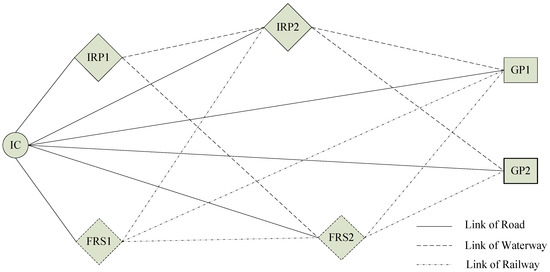
Figure 1.
The proposed port-hinterland intermodal transportation network. FRS, freight rail station; IRP, inland river port; IC, inland city; GP, gateway seaport.
With the concern for the greenness, the economic objective and environmental goal are the main focuses and they are integrated for the purpose of trade-off relationship analysis and then finding green network distribution solutions. With regards to the symmetry, the economic and environmental objectives might come to a compromise in these solutions. Thus, the optimization problem in this study is to obtain green freight distribution solutions through the proposed network under the given transportation demands in inland cities and some capacity restrictions, in which the choice of transport routes, the selection of gateway ports, and network flow distribution are determined by the competition in economic and environmental objectives.
This is not a standard hub-spoke network design problem, as it is assumed that there could be direct links from inland city origin to gateway seaport destination and the inland city nodes also can be assigned to more than one inland intermodal terminal. On top of that, it is also assumed that the transshipments and connections of transportation modes only occur at inland intermodal terminals. The number, type, and maximum container handling capacity of inland intermodal nodes are known. Thus, these assumptions increase the number of possible routes from origin to destination, and thus better reflect reality as they allow hybrid inter-terminal connections by rail–barge, barge–rail, barge–barge, and rail–rail intermodal options, especially for the case of long-range freight transportation.
Moreover, in the actual port-hinterland container transportation system, the transportation demand for each inland city is uncertain, and it is also difficult to determine the accurate probability distribution of demand through historical data. Therefore, this study additionally assumes that the specific probability distribution of transportation demand is unknown and only some distribution information such as the mean and variance of demand parameter is given. Although there are different categories of goods for foreign trade and different types of loading containers, the freight unit of TEU (twenty-foot equivalent unit) is applied for the consideration of unification and the freight export direction is mainly focused on in this study. In view of this, a distributionally robust optimization approach with chance constraint, which ensures that the uncertain transportation demand can be satisfied under the worse-case distribution condition, is applied to address the uncertainty. It could help analyze the performance of the port-hinterland transportation network on economic and environmental objectives and their trade-off relationships under different lower bounds of the probability for the chance constraint. The impacts of uncertain transportation demands on the green port-hinterland freight distribution network optimization can also be further explored.
2.2. Notations
The set of index, decision variables and input parameters for the model are listed in Table 1, Table 2 and Table 3 respectively.

Table 1.
The list of index set.
Table 2.
The list of decision variables.
Table 3.
The list of input parameters.
As for the mathematical expression, refers to the trace of matrix and , which is denoted by . implies that is positive semi-definite. Given the mean and variance of uncertain demand, the matrix of second-order moment can be expressed as , in which is the second-order moment and is the sum of the squares of the mean and variance (). When , is positive definite ().
2.3. Model Formulation
The economic objective and environmental objective of proposed transportation network are measured by the total logistics costs and the total CO2 emissions of the network, respectively. The former includes the transportation costs on the transportation routes and the handling as well as storage costs at the inland intermodal terminals. The latter consists of the corresponding route emissions and terminal handling CO2 emissions. A bi-objective optimization model for the port-hinterland container intermodal transportation network with chance constraint can be constructed as follows:
Equations (1) and (2) are objective functions representing the minimum total logistics costs of the network and the minimum total CO2 emissions of the network, respectively. Constraint (3) is the chance constraint, which ensures that the total amount of goods transported from inland city to all seaports meets the worst distribution of the transportation demand of each city. Constraint (4) indicates that the quantity of containers routed from the city to the assigned intermodal terminal is the sum of the volume through road–rail or road–waterway intermodal transportation and the volume through inter-terminal transportation. Constraint (5) ensures the balance of goods entering and leaving the inland intermodal terminals. Constraints (6) and (7) are the container handling capacity limitations of inland intermodal terminals and gateway seaports, respectively. Constraints (8)–(10) are non-negative integer constraints of decision variables.
2.4. Model Transformation
As the model contains the distributionally chance constraint, which is difficult to solve, we can first transform it into the corresponding Lagrange equivalent problem. Then, it is further transformed into a semi-definite programming problem through classified discussion. Finally, it can be transformed into a mixed integer linear optimization equivalent problem, which is easy to solve.
For distributionally robust chance Constraint (3), because , so and Constraint (3) is equivalent to Equation (11).
Lemma 1.
The following problem (12) is equivalent to Equation (11)
Proof.
An indicative function [27] is defined as follows:
Introducing the indicative function into Equation (11), can be expressed as follows:
The Lagrange function is defined as follows:
where is the variable matrix of Lagrange product term. Because , the strong duality holds.
Let , the problem (14) is then equivalent to (16):
where
In other words, only if , is finite.
As for , there are two situations:
- (1)
- , for any ;
- (2)
- , for any , which satisfies .
Situation 1 is equivalent to ; situation2 is valid only if there exists , which makes and
Therefore, problem (14) is equivalent to (18):
In other words, Equation (11) is equivalent to the problem (12). □
Theorem 1.
Constraint (3) with worst-case probability can be approximated from the following constraint:
Proof.
It can be seen from problem (18) that the optimal value is available when . We divide (12) by at both sides of the formula and then replace and with a new and new , respectively. Then, (12) can be represented by (20):
Owing to the equivalent relationship between the following formulas according to [27],
- (1)
- ;
- (2)
- there is asymmetric matrix and , which means that
Thus, we can obtain that distributionally robust chance Constraint (3) is equivalent to (19). □
To solve the bi-objective model, the ε-constraint method is adopted by selecting one of objectives as the main goal and converting another objective into an additional constraint. In this paper, costs minimization is selected as the main goal and network emissions formula is added as additional constraint. Therefore, after the transformation approach on the chance constraint above, the bi-objective optimization problem can be then reformulated as following:
s.t.
2.5. Model Solution
The trade-off relationships between total cost and total emissions as well as the Pareto frontier under a certain probability level of chance constraint can be obtained by applying the ε-constraint method, in which a range of network emissions limitations (ε) according to different emissions reduction percentages is set, while minimizing the total costs of the transportation network is selected as the main objective. The model in each ε setting is solved with the software of CPLEX solver to obtain the numerical results of network cost, network emissions, and modal split. After that, various probability levels are proposed in the model and the above-mentioned process is repeated.
3. Case Study
3.1. CaseDescription and Data Collection
The Yangtze River Economic Belt in China is known worldwide because of the Yangtze River golden waterway. It is the longest inland river in Asia and connects the eastern, central, and western parts of China. The port-hinterland container intermodal transportation system of the Yangtze River Economic Belt completes most of the foreign containerized cargo transportation through Shanghai Port and Ningbo-Zhoushan Port. They rank first and fourth in container traffic, respectively [28], and increasing container volume worldwide is forcing them to improve hinterland connections. In this paper, they are recognized as gateway seaports for the proposed port-hinterland intermodal transportation network and 72 inland cities are selected as the freight transportation demand generation nodes according to their importance in the aspects of population scale, economic scale, and foreign volume. As for inland intermodal terminals in the Yangtze River Economic Belt, several river ports that can process substantial containers have developed well in the past decades, while the container railway stations only witnessed growth in volume in the past years. As for the data source, Table 4 gives the mean and standard deviation of transportation demand of each inland city, which are estimated by the authors. The container handling capacity of inland intermodal terminals and gateway seaports are shown in Table 5. Transportation costs per TEU from node to node are gathered from third logistics firms, China Railway Service Center website, and Changjiang Waterway Bureau website. CO2 emissions rate varies from country to country and the work of Die Zhang [29], which reflects the emissions situation of inland transportation activities in China, is referred in this paper. The carbon emissions factor of each transportation mode is shown in Table 6. The carbon emissions factor for transshipment at inland intermodal terminals is estimated as 5.8 kg/TEU, according to China Port Yearbook.
Table 4.
The mean and standard deviation of transportation demand of inland cities (unit: twenty-foot equivalent unit (TEU)).
Table 5.
Container handling capacity at terminals and seaports (103 TEUs).
Table 6.
Carbon emissions factors of transportation modes (Unit: kg/(TEU∙km)).
3.2. Experimental Results
3.2.1. Results in Different Objective Optimization and Trade-Off Relationship Analysis ()
The model is firstly computed and runs with different optimization goals (costs minimization only, emissions minimization only and bi-objective optimization) by inputting parameters mentioned in Section 3.1 under the probability level of chance constraint with 0.90. Table 7 gives the model outputs on total network costs, network emissions, and flow distribution of the port-hinterland intermodal transportation network in the Yangtze River Economic Belt under three optimization objectives. In the costs minimization model, the lowest network cost that the transportation network of the Yangtze River Economic Belt could achieve is 3255.6 million dollars and the corresponding network emissions is 4.448 million tons. When the optimization objective is network emissions, the minimumCO2 emissions that the transportation network could achieve is 3.238 million tons, which is approximately 27.2% lower than the network emissions in the lowest cost model, and the corresponding total network cost is 3511.2 million dollars.
Table 7.
Results of total costs, total emissions, and flow distribution with different optimization objectives ().
When it comes to the bi-objective optimization model, Figure 2 depicts the Pareto frontier of cost goal and emissions goal in detail, which shows the trade-off relationship between total costs and total emissions. As shown in Figure 2, after the limitation percentage of 85.0% on network emissions, maintaining the same percentage of emissions reduction requires a greater network cost increase. It indicates that the 85.0% limitation level would be a watershed between the cost target and emissions target. The numerical results at this level are also listed in Table 7. At this point, the network costs and network emissions reach a compromise in the trade-off relationships. In other words, the transportation network not only could achieve considerable emissions reduction at this emission limitation level, but also could avoid the substantial increase in total logistics costs through the network.
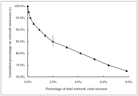
Figure 2.
Pareto Frontier between total costs and total emissions ().
It can also be found that the cost goal and emissions reduction present opposite trends for the case in the Yangtze River Economic Belt. With the decrease of the limitation on network emissions (ε), the emissions reduction percentage increases, while the total network cost trend keeps growing.
Through careful examination, it can be noticed that, in the three optimization models, the proportion of direct road transportation is always the highest, while the usage rates of intermodal transportation alternatives are relatively low. This also can be found from the difference in flow distribution in Table 7. This is because, in the actual case of the Yangtze River Economic Belt, many inland cities have road links to gateway seaports, while they do not have barge shipping lines or railway trains to seaports. With the tightening of the emissions limitation, the flow market of rail intermodal transportation increases obviously while that of barge intermodal and inter-terminal transportation decrease. This implies that the choice of intermodal transport alternatives in the Yangtze River Economic Belt is restricted by the trade-offs between costs and emissions.
3.2.2. Sensitivity Analysis of Probability Levels of Chance Constraint
In order to investigate the effects of different probability levels of chance constraint on the bi-objective optimization decision of port-hinterland transportation network, the model results under the lower bounds of the probability of 0.8, 0.85, 0.9, 0.95, and 0.98 for the chance constraint of transportation demand are all calculated and their Pareto frontier graphs are depicted in Figure 3. It can be found that the model obtains different Pareto optimal solutions under various probability levels of chance constraint for transportation demand, as shown in Figure 3. With the increase of the lower bound of probability for chance constraint, the Pareto frontier moves forward and total costs and total emissions are both on the rise. This indicates that the performance of network costs and network emissions of the transportation network can be influenced by the lower bound of probability. In addition, the higher the required lower bound of probability for chance constraint, the greater the impact brought about.
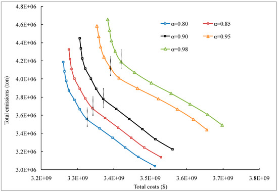
Figure 3.
Trends of Pareto frontier between total costs and total emissions under different settings on .
As for the trade-offs between two targets under different probability levels of chance constraint, the Pareto frontier also varies remarkably. When higher requirements for the lower bound of probability are put forward, the trend of Pareto frontier tends to be gentler, as shown in Figure 3. Especially at the probability level of 0.95 and 0.98, the slope of the Pareto frontier drops more prominently than that at lower probability levels (0.80, 0.85, and 0.90). This means that the cost to achieve emission reduction targets for the case in Yangtze River Economic Belt becomes higher and the compromise solution between two objectives is also more difficult to obtain. Therefore, when the required lower bound of probability for chance constraint of transportation demand is high, there exists a great impact on the trade-off relationship between network costs and network emissions.
Further, Figure 4 investigates the comparison of flow distribution of each compromise solution in bi-objective optimization under different probability levels of chance constraint. It is also the reason why the trade-offs between cost target and emissions target change, as depicted in Figure 3. As shown, there is nearly no difference in flow distribution at low probability levels of 0.8, 0.85, and 0.9. However, when the high lower bound of probability for chance constraint is required, such as 0.95 and 0.98, flows on direct road climb up, while intermodal flows decrease to different degrees. This is because the inland terminal capacity of handling container transshipment has become saturated. Thus, if the high lower bound of probability for chance constraint is required for the port-hinterland transportation network in the Yangtze River Economic Belt, it would be better to expand the handling capacity of inland intermodal terminals.
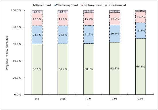
Figure 4.
The comparison of network flow distribution under different settings on .
4. Discussion
This paper differs from the previous literature in two aspects. Firstly, hybrid intermodal transportation alternatives are encompassed to help analyze the greenness of hinterland transportation network. Secondly, a distributionally robust chance constrained approach is introduced with the partial distributional information of mean and variance for the uncertain demand, and then trade-offs between economic and environmental goals are investigated by incorporating the variation in lower bound of probability for chance constraint.
The flow distribution results indicate that railway–road intermodal transport can be promoted with the greenness requirement on the proposed port-hinterland transportation network. In other words, more flows are absorbed to the railway–road intermodal routes when the optimization objective is the bi-objective case or the CO2 minimum emissions case. It is an interesting finding for intermodal freight transport, because it implies that there is competition in hybrid intermodal transportation alternatives, rather than the only competition in unimodal and single intermodal options in most intermodal transport research articles (such as the works of Crainic et al. [5], Santoset al. [13], and Bouchery and Fransoo [30]). This finding might provide a different perspective for the port-hinterland intermodal transportation network optimization with the greenness consideration.
As for the uncertainty of transportation demand in port-hinterland freight network optimization, this study considers the situation that the accurate distribution formation of stochastic variation is usually difficult to obtain in reality. In recent literature, most studies on hinterland freight transportation network planning traded the transportation demand as the determined parameter or stochastic parameter with the known distribution (such as the works of Dai et al. [31], Liu et al. [32], and Chen and Wang [33]. For this case, a distributionally robust chance constrained approach is introduced and a tractable approximation of the chance constrained problem is then developed to reformulate the model as a deterministic linear programming. The results indicate that the green solution under bi-objective optimization model for the port-hinterland transportation system is more difficult to obtain with the higher requirement of lower bound of probability for chance constraint of transportation demand. It also offers a different perspective for the green port-hinterland intermodal transportation network optimization with the uncertainty of transportation demand.
5. Conclusions
This paper models the uncertainty in green port-hinterland intermodal transportation network optimization through a distributionally robust chance constrained method and a bi-objective approach. The chance constraint that transportation demand is satisfied under the worst-case distribution situation is proposed based on the mean and variance of probability distribution for uncertain demand. The approaches of equivalent transformation on chance constraint and ε-constraint method are employed to help reformulate the model.
The trade-offs between network costs and network emissions are analyzed and the sensitivity of probability levels for chance constraint on Pareto frontier is followed by an application of the port-hinterland intermodal transportation network in the Yangtze River Economic Belt in China. The results show that network costs and network emissions both increase significantly with the increase of the lower bound of probability for chance constraint. When the probability level climbs to some high values, the movement of Pareto frontier changes a lot, which indicates that the probability level has a great impact on the trade-offs between network costs and network emissions. This also implies that it is better to expand the handling capacity of inland intermodal terminals at high probability levels for chance constraint. Overall, the approach of distributionally robust chance constraint in the model provides a novel insight to solve the dynamic planning problem caused by the fluctuation of demands in real life. The decision makers can also choose an appropriate solution according to their preference for economic and environmental aspects.
Although the study of this paper provides some decision supports for the green port-hinterland container transportation network with uncertain demand, it also has a lack of consideration of more uncertain parameters in the model. For example, transportation cost, carbon emissions, and terminal handling capacity may all face uncertainty in the real-world case. Thus, further research might extend uncertain programming in the green logistics network in a more comprehensive direction.
Author Contributions
Conceptualization, Q.D.; Investigation, Q.D.; Methodology, Q.D.; Resources, J.Y.; Software, Q.D.; Supervision, J.Y.; Writing—original draft, Q.D.; Writing—review & editing, J.Y. All authors have read and agreed to the published version of the manuscript.
Funding
The authors would like to thank the financial supports from Jilin Province Transportation Science and Technology Plan Project (46160101).
Acknowledgments
The first author is grateful to the support of China Scholarship Council for the joint Doctoral Program with one-year period in University of Liverpool of UK.
Conflicts of Interest
The authors declare no conflict of interest.
References
- Notteboom, T. The relationship between seaports and the intermodal hinterland in light of global supply chains: European challenges. In Port Competition and Hinterland Connections; Round Table 143; OECD Publishing: Paris, France, 2009; p. 30. [Google Scholar]
- OECD/ITF. Port Competition and Hinterland Connections; OECD Publishing: Paris, France, 2009; ISBN 9789282102244. [Google Scholar]
- Woxenius, J. Generic framework for transport network designs: Applications and treatment in intermodal freight transport literature. Transp. Rev. 2007, 27, 733–749. [Google Scholar] [CrossRef]
- Frémont, A.; Franc, P. Hinterland transportation in Europe: Combined transport versus road transport. J. Transp. Geogr. 2010, 18, 548–556. [Google Scholar] [CrossRef]
- Crainic, T.G.; Dell’Olmo, P.; Ricciardi, N.; Sgalambro, A. Modeling dry-port-based freight distribution planning. Transp. Res. Part C Emerg. Technol. 2015, 55, 518–534. [Google Scholar] [CrossRef]
- Caris, A.; Limbourg, S.; Macharis, C.; Van Lier, T.; Cools, M. Integration of inland waterway transport in the intermodal supply chain: A taxonomy of research challenges. J. Transp. Geogr. 2014, 41, 126–136. [Google Scholar] [CrossRef]
- European Commission White Paper. Roadmap to a Single European Transport Area—Towards a Competitive and Resource Efficient Transport System.2011. Available online: https://eur-lex.europa.eu/legal-content/EN/ALL/?uri=CELEX:52011DC0144 (accessed on 12 October 2017).
- Caris, A.; Macharis, C.; Janssens, G.K. Decision support in intermodal transport: A new research agenda. Comput. Ind. 2013, 64, 105–112. [Google Scholar] [CrossRef]
- Macharis, C.; Van Hoeck, E.; Pekin, E.; Van Lier, T. A decision analysis framework for intermodal transport: Comparing fuel price increases and the internalisation of external costs. Transp. Res. Part. A Policy Pract. 2010, 44, 550–561. [Google Scholar] [CrossRef]
- Macharis, C.; Caris, A.; Jourquin, B.; Pekin, E. A decision support framework for intermodal transport policy. Eur. Transp. Res. Rev. 2011, 3, 167–178. [Google Scholar] [CrossRef]
- Mostert, M.; Caris, A.; Limbourg, S. Road and intermodal transport performance: The impact of operational costs and air pollution external costs. Res. Transp. Bus. Manag. 2017, 23, 75–85. [Google Scholar] [CrossRef]
- Iannone, F. The private and social cost efficiency of port hinterland container distribution through a regional logistics system. Transp. Res. Part. A Policy Pract. 2012, 46, 1424–1448. [Google Scholar] [CrossRef]
- Santos, B.; Limbourg, S.; Carreira, J.S. The impact of transport policies on railroad intermodal freight competitiveness—The case of Belgium. Transp. Res. Part D: Transp. Environ. 2015, 34, 230–244. [Google Scholar] [CrossRef]
- Zhang, M.; Janic, M.; Tavasszy, L. A freight transport optimization model for integrated network, service, and policy design. Transp. Res. Part. E Logist. Transp. Rev. 2015, 77, 61–76. [Google Scholar] [CrossRef]
- Lam, J.S.L.; Gu, Y. A market-oriented approach for intermodal network optimisation meeting cost, time and environmental requirements. Int. J. Prod. Econ. 2016, 171, 266–274. [Google Scholar] [CrossRef]
- Demir, E.; Hrušovský, M.; Jammernegg, W.; Van Woensel, T. Green intermodal freight transportation: Bi-objective modelling and analysis. Int. J. Prod. Res. 2019, 57, 6162–6180. [Google Scholar] [CrossRef]
- Contreras, I.; Cordeau, J.; Laporte, G. Stochastic uncapacitated hub location. Eur. J. Oper. Res. 2011, 212, 518–528. [Google Scholar] [CrossRef]
- Ardjmand, E.; Young, W.A.; Weckman, G.R.; Bajgiran, O.S.; Aminipour, B.; Park, N.; Ii, W.A.Y. Applying genetic algorithm to a new bi-objective stochastic model for transportation, location, and allocation of hazardous materials. Expert Syst. Appl. 2016, 51, 49–58. [Google Scholar] [CrossRef]
- Wang, X. Stochastic resource allocation for containerized cargo transportation networks when capacities are uncertain. Transp. Res. Part. E Logist. Transp. Rev. 2016, 93, 334–357. [Google Scholar] [CrossRef]
- Zhao, Y.; Xue, Q.; Cao, Z.C.; Zhang, X. A Two-stage chance constrained approach with application to stochastic intermodal service network design problems. J. Adv. Transp. 2018, 2018, 1–18. [Google Scholar] [CrossRef]
- Karoonsoontawong, A.; Waller, S.T. Robust dynamic continuous network design problem. Transp. Res. Rec. 2007, 2029, 58–71. [Google Scholar] [CrossRef]
- Sun, H.; Gao, Z.; Long, J.C. The robust model of continuous transportation network design problem with demand uncertainty. J. Transp. Syst. Eng. Inf. Technol. 2011, 11, 70–76. [Google Scholar] [CrossRef]
- Ng, M.; Lo, H.K. Robust models for transportation service network design. Transp. Res. Part. B Methodol. 2016, 94, 378–386. [Google Scholar] [CrossRef]
- Scarf, H.E. A min-max solution of an inventory problem. Herbert Scarf’s contributions to economics. Int. J. Game Theory Res. 1958, 6, 19–27. [Google Scholar]
- Yin, F.; Chen, Y.; Song, F.; Liu, Y. A new distributionally robust p-hub median problem with uncertain carbon emissions and its tractable approximation method. Appl. Math. Model. 2019, 74, 668–693. [Google Scholar] [CrossRef]
- Gourtani, A.; Nguyen, T.D.; Xu, H. A distributionally robust optimization approach for two-stage facility location problems. EURO J. Comput. Optim. 2020, 8, 141–172. [Google Scholar] [CrossRef]
- El Ghaoui, L.; Oks, M.; Oustry, F. Worst-case value-at-risk and robust portfolio optimization: A conic programming approach. Oper. Res. 2003, 51, 543–556. [Google Scholar] [CrossRef]
- World Shipping Council. Top 50 World Container Ports. Available online: http://www.worldshipping.org/about-the-industry/global-trade/top-50-world-container-ports (accessed on 2 May 2018).
- Zhang, D. Study on the Container Port Inland Transportation System’s Network Optimization with Low Carbon Theory. Dalian Maritime University, 2015. Available online: http://kns.cnki.net/KCMS/detail/.detail.aspx?dbcode=CMFD&dbname=CMFD201601&filename=1015656920.nh&v=MTM3NjNMdXhZUzdEaDFUM3FUcldNMUZyQ1VSTEtmYitSbkZ5L2dXNy9OVkYyNkc3VzlHTmpPcjVFYlBJUjhlWDE= (accessed on 23 October 2018).
- Bouchery, Y.; Fransoo, J. Cost, carbon emissions and modal shift in intermodal network design decisions. Int. J. Prod. Econ. 2015, 164, 388–399. [Google Scholar] [CrossRef]
- Dai, Q.; Yang, J.; Li, D. Modeling a three-mode hybrid port-hinterland freight intermodal distribution network with environmental consideration: The case of the yangtze river economic belt in China. Sustainability 2018, 10, 3081. [Google Scholar] [CrossRef]
- Liu, K.; Li, Q.; Zhang, Z.H. Distributionally robust optimization of an emergency medical service station location and sizing problem with joint chance constraints. Transp. Res. Part. B Methodol. 2019, 119, 79–101. [Google Scholar] [CrossRef]
- Chen, X.; Wang, X. Effects of carbon emission reduction policies on transportation mode selections with stochastic demand. Transp. Res. E Logist. Transp. Rev. 2015, 90, 196–205. [Google Scholar] [CrossRef]
© 2020 by the authors. Licensee MDPI, Basel, Switzerland. This article is an open access article distributed under the terms and conditions of the Creative Commons Attribution (CC BY) license (http://creativecommons.org/licenses/by/4.0/).