The Effect of a Non-Local Fractional Operator in an Asymmetrical Glucose-Insulin Regulatory System: Analysis, Synchronization and Electronic Implementation

Abstract

For studying biological conditions with higher precision, the memory characteristics defined by the fractional-order versions of living dynamical systems have been pointed out as a meaningful approach. Therefore, we analyze the dynamics of a glucose-insulin regulatory system by applying a non-local fractional operator in order to represent the memory of the underlying system, and whose state-variables define the population densities of insulin, glucose, and $\beta$-cells, respectively. We focus mainly on four parameters that are associated with different disorders (type 1 and type 2 diabetes mellitus, hypoglycemia, and hyperinsulinemia) to determine their observation ranges as a relation to the fractional-order. Like many preceding works in biosystems, the resulting analysis showed chaotic behaviors related to the fractional-order and system parameters. Subsequently, we propose an active control scheme for forcing the chaotic regime (an illness) to follow a periodic oscillatory state, i.e., a disorder-free equilibrium. Finally, we also present the electronic realization of the fractional glucose-insulin regulatory model to prove the conceptual findings.

1. Introduction

Homeostasis is the tendency of organisms to auto-regular and maintain their internal environment in a stable state [1], For instance, an excellent model to describe the homeostatic process in the organism is the glucose-insulin system [1,2]. On one side, when the glucose level is low, arises diverse pathologies (anxiety, tremors, obfuscation, coma, etc.). On the other side, microvascular damages in the retina, kidney, and neuronal injuries, which lead to chronic renal insufficiency and blindness, are originated by high glucose concentrations. The principal pathology of glucose homeostasis is diabetes. Diabetes can be stated as a chronic disorder provoked when the pancreas does not produce insulin in enough quantities, and also if the body cannot successfully process it, resulting in atypical high blood sugar levels. Because of the autoimmune annihilation of $\beta$-cells, the insulin released by the pancreas to the human organism is not enough to maintain a certain healthy level, and therefore, the Type 1 Diabetes Mellitus (T1DM) may be manifested. On the contrary, when the beta-cells can produce supranormal, or average concentrations of insulin, but cannot be adequately used in reducing glycemia, the Type 2 Diabetes Mellitus (T2DM) appears [3].

Health agencies [4] demonstrate people, mainly adults, living with diabetes has almost quadrupled from 1980 to 422 million. This rise is primarily due to the rise in T2DM and factors driving it, including overweight and obesity. Diverse mathematical models using ODEs and OdEs have provided a common path to understand multiple complex systems [5,6]. In the last years, because of the long-memory of fractional-order operators, fractional-order systems have gained extensive attention for describing and understanding physical and biological systems [5,7,8,9,10]. For instance, the analysis of diverse biological systems, such as bio-impedance, drug diffusion, respiratory tissue, and so forth, was reported in [11] using fractional calculus. In [12], the authors characterize the trade-offs between HIV infection and the tumor-immune system employing fractional-order biological systems. Kheiri and Jafari [13] formulated a fractional-order theory that was focused on the multi-patch HIV/AIDS model to analyze whether human migration has effects on the propagation of the HIV/AIDS outbreak. In [14], the authors reported a fractional-order Izhikevich system to obtain insights on distinct neuronal spike responses, including bursting, fast-, regular-spiking, and chattering, as the no-integer order varies. The functioning at electrical level of a fractional-order system of an isolated $\beta$-cell is presented in [15,16]. In [17], was reported the comparison among diverse scenarios, such as integer, constant, no-constant and fractional-order derivatives, in order to explain the memory index. In [18], the transmission issues of a susceptible-infected-recovered model were analyzed. They found a proper yield of memory of the fractional-order systems to forecast the pandemic spread. Finally, [19] discovered that the neuron’s firing rate could be emulated with a fractional derivative and a slowly varying of the parameters. Therefore, the unique rat neocortical pyramidal neurons have several time-scales.

Therefore, the study of fractional-order biological models continues been critical for an accurate analysis of several health conditions, as well as being essential to understanding this significant open-topic.

Additionally, the synchronization and collective dynamics play an essential role both in physical [20,21,22] and biological systems [15,23,24,25,26]. By one side, the synchronization is necessary for systems with stable behavior, for instance, the human heartbeat and respiration [27,28]; nevertheless, on the other hand, the synchronized state could provoke severe pathologies such as the Parkinson’s disease where the excessive synchronization correlates with a motor deficit. For the glucose-insulin regulatory system, a synchronization state is mandatory, since this condition is closely related to a disorder-free state where the glucose-insulin concentrations synchronize. In [29], the $\beta$-cell synchronization is fundamental to effectuate a pulsatile insulin liberation, which carries more substantial hypoglycemic results compared to constant secretion. In [30], the synchronization between gap-junctions and adjacent cells is essential to limit the heterogeneity and biological noise, thence obtaining a robust activation of the $\beta$-cells population within the islet. Pecora and Carroll in [31] showed that two nonlinear dynamical systems could be synchronized by introducing appropriate coupling, since then, a variety of approaches were proposed to deal with synchronized states of fractional-order chaos generators, and these include backstepping, adaptive, and active controls [32,33]. Regarding the chaos synchronization applying the active control method [34], it has been demonstrated that an active controller can be straightforwardly designed to achieve synchronization globally if the nonlinearity of the system is known. Thereupon, it is considered to be a promising control strategy due to its straightforwardness. [33].

In addition, the experimental verification of fractional-order models is a topic that has been attracting the attention of researchers [35,36,37,38,39]. In this scenario, ARM-based embedded systems have become in a central block integrated with non-embedded technologies, such as FPGAs, DSPs, and microcontrollers. Subsequently, now it is possible to implement complex software and hardware functionality on a single chip [40]. Several digital hardware have been reported and verified contemplating integer-order chaotic systems [41,42,43]. Notwithstanding, just a short-list of papers have studied the implementation of fractional chaos oscillators on ARM platforms [44,45].

Motivated by the discussion mentioned above, we analyze the effect of a non-local fractional operator in an asymmetrical glucose-insulin regulatory system. More specifically, the system parameters that were related to hypoglycemia, hyperinsulinemia, T1DM, and T2DM, were studied by using both analytical (stability of equilibrium) and numerical (bifurcation diagrams and basins of attraction) techniques. Additionally, we found that the system presents a chaotic attractor, as demonstrated by its phase portraits and Lyapunov exponent spectrum. Besides, the theoretical insights of the glucose-insulin interaction can be validated by using the proposed electronic implementation based on the embedded SoC ARM Broadcom BCM2837B0. Latter, the synchronization between a chaotic behavior (disorder) and periodic behaviors (average condition) were achieved by applying a simple control strategy.

The sections of the manuscript contain the following. The fractional-order glucose-insulin system, in the sense of Caputo, is presented in Section 2. The stability of the equilibrium points is analyzed in Section 3. Several dynamical analysis for the hypoglycemia, hyperinsulinemia, T1D, and T2D are presented in Section 4. Two synchronization schemes using the active control approach are introduced in Section 5. The ARM implementation is carried out in Section 6, which is followed by the conclusions in Section 7.

2. Fractional-Order Glucose-Insulin Regulatory System

Because diverse biological systems present memory effects, direct generalization maybe by applying fractional-order differential equations, i.e., arbitrary (non-integer) orders. In this manner, we can get a closer insight into the real phenomena. The benefits of fractional-order are mainly to capture the entire time evolution for physical processes, being a kind of memory index, as well as more degrees of freedom for the resulting models. The analysis conducted in this work is inspired by the glucose-insulin regulatory system in [46], as given in Equation (1). This model was derived from the Ackerman, Bajaj, and Rao, and predator-prey Volterra models. As a consequence, the resulting system is formulated as the trade-off relating the glucose and insulin, but including the beta-cells interaction. Apart from normal metabolic conditions described by the classical relation between prey (glucose) and predator (insulin), the model (1) also characterizes the metabolic disorders as chaotic oscillations. Abnormal biological conditions, including glucose-insulin interactions, can be stated as chaotic evolutions of the dynamical systems, as given in [47,48,49,50], to mention a few. From experimental data, Ref. [51] also discussed that the T1DM may have chaotic behaviors. In this manner, the proposed analysis of the glucose-insulin regulatory system is in the same line of previous studies, but instead applying fractional-calculus theory.

$$\begin{array}{ccc}\hfill \dot{x}& =& -a_{1}x+0.1xy+1.09y^2-1.08y^3+0.03z-0.06z^2+a_7{z}^3-0.19,\hfill \\ \hfill \dot{y}& =& -a_{8}xy+3.84x^2+1.2x^3+0.3y(1-y)-1.37z+0.3z^2-0.22z^3-0.56,\hfill \\ \hfill \dot{z}& =& a_{15}y-1.35y^2+0.5y^3+0.42z+0.15yz,\hfill \end{array}$$

(1)

we now introduce a fractional-order version [52], but instead applying the Caputo’s definition. Let us consider the fractional differential operator $D^{q}f\left(t\right)=J^{n-\gamma }{D}^{n}f\left(t\right)$, with $q>0$ and $n\in \mathbb{N}$, where $D^n$ describes the n-order derivative, while $J^{\gamma }$ defines the $\gamma$-order integral operator in the sense of Riemann-Liouville as

Definition 1.

For a function $f\left(t\right)$, the fractional-order (γ) integral, with $\gamma \in {\mathbb{R}}^{+}$ can be determined by

$$J^{\gamma }f\left(t\right)=\frac{1}{\mathsf{\Gamma }\left(\gamma \right)}{\int }_{t_0}^t{(t-s)}^{\gamma -1}f\left(s\right)ds,$$

(2)

where $t\ge t_0$ and $\mathsf{\Gamma }(·)$ is the Gamma function, defined as $\mathsf{\Gamma }\left(s\right)={\int }_0^{\infty }{t}^{s-1}{e}^{-t}dt$.

In this manner, the Caputo operator of fractional-order can be established by

Definition 2.

The fractional derivative of Caputo with order q for a function $f\left(t\right)\in {\mathbb{C}}^n([t_0,\infty ),\mathbb{R})$ is given as

$$D^{q}f\left(t\right)=\frac{1}{\mathsf{\Gamma }(n-q)}{\int }_{t_0}^t\frac{f^{\left(n\right)}\left(s\right)}{{(t-s)}^{q-n+1}}ds,$$

(3)

and when $0<q<1$ is given, as follows

$$D^{q}f\left(t\right)=\frac{1}{\mathsf{\Gamma }(1-q)}{\int }_{t_0}^t\frac{f^{{}^{\prime }}\left(s\right)}{{(t-s)}^q}ds.$$

(4)

By substituting Equation (4) in Equation (1), we get the fractional-order glucose-insulin regulatory system that is given by

$$\begin{array}{ccc}\hfill D^{q_1}x& =& -a_{1}x+0.1xy+1.09y^2-1.08y^3+0.03z-0.06z^2+a_7{z}^3-0.19,\hfill \\ \hfill D^{q_2}y& =& -a_{8}xy+3.84x^2+1.2x^3+0.3y(1-y)-1.37z+0.3z^2-0.22z^3-0.56,\hfill \\ \hfill D^{q_3}z& =& a_{15}y-1.35y^2+0.5y^3+0.42z+0.15yz,\hfill \end{array}$$

(5)

where $D^{q_i}(x,y,z)$ with $i=1,2,3$ is the the fractional derivative operator in Caputo’s sense [53], $q_i$ is the fractional-order satisfying $0<q_i\le 1$, $(x,y,z)$ describe the population density of insulin, the population size of glucose, and the population size of $\beta$-cells, respectively. The representative reduction of insulin levels for glucose deficiency is described by $a_1$, whereas the parameter $a_8$ stands for the impact of insulin on glucose. Additionally, the increment rate of insulin concentrations released by b-cells is provided by $a_7$. Finally, the increasing rate of the $\beta$-cells provoked, when the glucose levels also grow, is given by $a_{15}$ [46]. From the nature of how this system was conceived, the parameters must be nonnegative [46].

The discrete-time version for the proposed system (5) is set as:

$$\begin{array}{c}\hfill x_{n+1}=x_0+\frac{h^{q_1}}{\mathsf{\Gamma }(q_1+2)}\left(f_1(x_{n+1}^p,y_{n+1}^p,z_{n+1}^p)+\sum _{k=0}^n{\alpha }_{1,k,n+1}{f}_1(x_k,y_k,z_k)\right),\\ \hfill y_{n+1}=y_0+\frac{h^{q_2}}{\mathsf{\Gamma }(q_2+2)}\left(f_2(x_{n+1}^p,y_{n+1}^p,z_{n+1}^p)+\sum _{k=0}^n{\alpha }_{2,k,n+1}{f}_2(x_k,y_k,z_k)\right),\\ \hfill z_{n+1}=z_0+\frac{h^{q_3}}{\mathsf{\Gamma }(q_3+2)}\left(f_3(x_{n+1}^p,y_{n+1}^p,z_{n+1}^p)+\sum _{k=0}^n{\alpha }_{3,k,n+1}{f}_3(x_k,y_k,z_k)\right),\end{array}$$

(6)

where

$$\begin{array}{c}\hfill x_{n+1}^p=x_0+\frac{1}{\mathsf{\Gamma }\left(q_1\right)}\sum _{k=0}^n{\beta }_{1,k,n+1}{f}_1(x_k,y_k,z_k),\\ \hfill y_{n+1}^p=y_0+\frac{1}{\mathsf{\Gamma }\left(q_2\right)}\sum _{k=0}^n{\beta }_{2,k,n+1}{f}_2(x_k,y_k,z_k),\\ \hfill z_{n+1}^p=z_0+\frac{1}{\mathsf{\Gamma }\left(q_3\right)}\sum _{k=0}^n{\beta }_{3,k,n+1}{f}_3(x_k,y_k,z_k),\end{array}$$

(7)

with

$${\alpha }_{i,k,n+1}=\left\{\begin{array}{cc}{n}^{q_i+1}-(n-q_i){(n+1)}^{q_i},k=0,\hfill & k=0\hfill \\ {(n-k+2)}^{q_i+1}+{(n-k)}^{q_i+1}-2{(n-k+1)}^{q+1},\hfill & 1\le k\le n,\hfill \\ 1,\hfill & k=n+1,\hfill \end{array}\right.$$

(8)

and

$${\beta }_{i,k,n+1}\frac{h^{q_i}}{q_i}\left({(n+1-k)}_i^q-{(n-k)}_i^q\right).$$

(9)

note that $x_0,y_0,z_0$ are the initial values for, $f_1(x,y,z)=-a_{1}x+0.1xy+1.09y^2-1.08y^3+0.03z-0.06z^2+a_7{z}^3-0.19$, $f_2(x,y,z)=-a_{8}xy+3.84x^2+1.2x^3+0.3y(1-y)-1.37z+0.3z^2-0.22z^3-0.56$ and $f_3(x,y,z)=a_{15}y-1.35y^2+0.5y^3+0.42z+0.15yz,$ whether $q_i=q$, $i=1,2,3$ the system is said to be commensurate then the convergence order is described as $|y\left(t_n\right)-y_n|=O\left(h^{min(2,1+q)}\right)$, $h\to 0$ [54,55,56].

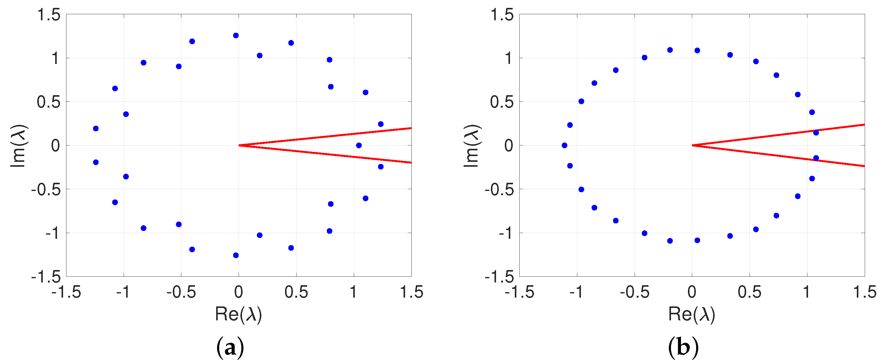
3. Stability Analysis of Fractional-Order Glucose-Insulin Model

A non-local differential equation with fractional-order $q\in (0,1)$, normally has a stability region larger than that of the integer-order version with $q=1$ [57]. We introduce the following theorems and definitions to discuss the stability of the proposed fractional-order system.

Definition 3.

A system denoted as

$$D^{q_i}{x}_i\left(t\right)=f_i(x_1\left(t\right),x_2\left(t\right),\dots ,x_n\left(t\right),t),x_i\left(0\right)=c_i,i=1,2,\dots ,n,$$

(10)

with trajectory $x\left(t\right)=0$, where $c_i$ are the starting conditions is $t^{-q}$ asymptotically stable if there is a nonnegative real q, so that:

$$\forall \left|\right|x\left(t\right)\left|\right|\mathrm{with}t\le t_0,\exists N\left(x\left(t\right)\right),\mathrm{such}\mathrm{that}\forall t>t_0,\left|\right|x\left(t\right)\left|\right|\le N{t}^{-q}.$$

Subsequently, fractional-order systems are known to have long memory, since they obey a behavior like $t^{-q}$, which slowly tends to 0 for the solutions x(t). A particular case of Mittag–Leffler stability is stated as power-law stability $t^{-q}$. [58,59].

Theorem 1.

Let a commensurate order system described by $D^{q}x=Ax$, with $x\left(0\right)=x_0$, $0<q<1$, $x\in {\mathbb{R}}^n$ and $A\in {\mathbb{R}}^{n\times n}$, is asymptotically stable if $|arg(\lambda \left)\right|>q\pi /2,$ is fulfilled for all eigenvalues of A. Besides, the critical eigenvalues fulfilling $|arg(\lambda \left)\right|=q\pi /2$ holding geometric multiplicity of one, where the geometric multiplicity of an eigenvalue is called the dimension of the subspace vectors v for $Av=\lambda v$ [60,61,62,63,64,65].

Theorem 2.

Let $D^{q}x=Ax,$ with $x\left(0\right)=x_0$ an incommensurate-order system, where $x={(x_1,x_2,\dots ,x_n)}^T\in {\mathbb{R}}^n$, $D^{q}x={(D^{q_1}{x}_1,D^{q_2}{x}_2,\dots ,D^{q_n}{x}_n)}^T,$$q_i\in {\mathbb{R}}^{+}$, $i=1,2,\dots ,n.$, $q_i\in (0,1)$, and $A=\left(a_{ij}\right)\in {\mathbb{R}}^{n\times n}$, $i=j=1,2,\dots ,n.$ By supposing w as the lowest common multiple of the denominators $u_i$’s of $q_i$’s, with $q_i=v_i/u_i$, $(u_i,v_i)=1$, $u_i,v_i\in {\mathbb{Z}}^{+}$ for $i=1,2,\dots ,n.$, the matrix of system is given by

$$\Delta \left(\lambda \right)=\left[\begin{array}{cccc}{\lambda }^{w{q}_1}-a_{11}& -a_{12}& \cdots & -a_{1n}\\ -a_{21}& {\lambda }^{w{q}_2}-a_{22}& \cdots & -a_{2n}\\ ⋮& ⋮& \ddots & ⋮\\ -a_{n1}& -a_{n2}& \cdots & {\lambda }^{w{q}_n}-a_{nn}\end{array}\right].$$

(11)

Therefore, the system $D^{q}x=Ax$ is globally asymptotically stable if the roots λ’s of its characteristic equation $det(\Delta (\lambda \left)\right)=0$ fulfil $|arg(\lambda \left)\right|>\pi /2w$, [60,61,62,63,64,65].

Theorem 3.

The equilibria $E_{*}$ with a instability measure defined as

$$\rho =(\pi /2w)-\underset{i}{min}\left\{\right|arg\left({\lambda }_i\right)\left|\right\},$$

(12)

is asymptotically stable if and only if (12) is defined nonpositive. Where ${\lambda }_i$’s are the roots of characteristic equation: $det(\mathrm{diag}\left([{\lambda }^{w{q}_1}{\lambda }^{w{q}_2}\cdots {\lambda }^{w{q}_n}]\right)-\partial f/\partial x{|}_{x=E_{*}})=0$, $\forall E_{*}\in \mathsf{\Omega }$ [64,65].

Remark 1.

If ρ is nonnegative, the underlying system can show a chaotic evolution since the equilibrium $E_{*}$ is unstable [64,65].

The first step consists of finding the equilibrium points of (5), which are calculated via $\mathbf{f}\left(\mathbf{x}\right)=0$, as follows

$$\begin{array}{ccc}\hfill 0& =& -a_{1}x+0.1xy+1.09y^2-1.08y^3+0.03z-0.06z^2+a_7{z}^3-0.19,\hfill \\ \hfill 0& =& -a_{8}xy+3.84x^2+1.2x^3+0.3y(1-y)-1.37z+0.3z^2-0.22z^3-0.56,\hfill \\ \hfill 0& =& a_{15}y-1.35y^2+0.5y^3+0.42z+0.15yz.\hfill \end{array}$$

(13)

Because of the biological interpretation of state variables [46], the stability analysis for $E^{*}=$$(x^{*},y^{*},z^{*})$ is only performed for nonnegative fixed points. Equation (5) has the following Jacobian

$$J=\left(\begin{array}{ccc}-a_1+0.1y*& 0.1x^{*}+2.18y^{*}-3.24y^{*2}& 0.03-0.12z^{*}+3a_7{z}^{*2}\\ -a_8{y}^{*}+7.68x^{*}+3.6x^{*2}& -a_{8}x+0.3(1-2y^{*})& -1.37+0.6z-0.66z^{*2}\\ 0& a_{15}-2.7y^{*}+1.5y^{*2}+0.15z& 0.42+0.15y^{*}\end{array}\right).$$

(14)

By setting $a_1=1.3$, $a_7=2.01$, $a_8=0.22$, $a_{15}=0.3$, we compute the equilibrium points and eigenvalues, as shown in

Table 1. Nonnegative equilibrium points and eigenvalues of the system (5).

${\mathit{E}}_{\mathit{i}}$	Equilibrium Point	Eigenvalues
$E_1$	$(0.802,1.853,1.286)$	${\lambda }_1=1.4652$, ${\lambda }_{2,3}=-1.4353\pm 7.7140i$
$E_2$	$(0.584,0.832,0.728)$	${\lambda }_1=-2.5327$, ${\lambda }_{2,3}=0.7664\pm 1.9699i$

. As can be noted, the system (5) has two nonnegative fixed points characterized for saddle points of index-1 and index-2, respectively. According to Theorem 1, chaos behavior may arise in the fractional-order glucose-insulin system when $|arg(\lambda \left)\right|>q\pi /2,$ holds. Therefore, the minimum commensurate fractional-order leading to chaotic oscillations is $q>0.7638$, which is remarkably lower than that reported in [52].

The chaotic attractor existence and local stability of the equilibria are presented below. The Jacobian matrix considering the equilibria $E_1$ and parameter $a_1$ is

$$J_{E_1}=\left(\begin{array}{ccc}-a_1+0.1853& -7.0110& 9.8541\\ 8.0788& -0.9887& -1.6903\\ 0& 0.6420& 0.6420\end{array}\right),$$

(15)

which generates the characteristic equation given, as follows

$$P\left(\lambda \right)={\lambda }^3+(a_1+b_1){\lambda }^2+(b_2{a}_1+b_3)\lambda +b_4{a}_1-b_5=0,$$

(16)

where $b_1=0.1054$, $b_2=0.2907$, $b_3=56.9826$, $b_4=0.395$, and $b_5=90.7232$, when considering the Routh–Hurwitz theory, obtaining the following conditions $a_1+b_1>0$, $b_2{a}_1+b_3>0$, and $b_4{a}_1-b_5>0$, which become in $a_1>-b_1$ and $b_3>-b_2{a}_1$, respectively. Due $b_5>b_4{a}_1$, there is a root positive which is unstable and a pair of complex conjugate with the negative real part. Thus $E_1$ is unstable being a saddle point of index 1.

The presence of a Hopf bifurcation in the system (5) at the equilibrium point $E_1$ is analyzed by replacing $\lambda =i\omega$ in (16) obtaining

$${\left(iw\right)}^3+(a_1+b_1){\left(i\omega \right)}^2+(b_2{a}_1+b_3)\left(i\omega \right)+b_4{a}_1-b_5=0,$$

(17)

then

$$-{\left(iw\right)}^3-(a_1+b_1){\omega }^2+(b_2{a}_1+b_3)\left(i\omega \right)+b_4{a}_1-b_5=0,$$

(18)

taking into account the real part of (18), therefore,

$${\omega }^2=\frac{b_5-b_4{a}_1}{-(a_1+b_1)},$$

(19)

because $a_1+b_1>0$, and $b_5,b_4,a_1>0$, hence ${\omega }^2<0$, so it is not possible, then, the equilibrium point $E_1$ does not suffer a Hopf bifurcation.

In order to study the stability of $E_1$ we consider the discriminant $D\left(P\right)$ of characteristic equation $P\left(\lambda \right)$, given as follows

$$D\left(P\right)=18d_1{d}_2{d}_3+{\left(d_1{d}_2\right)}^2-4d_3{d}_1^3-4d_2^3-27d_3^2,$$

(20)

where $d_1=(a_1+b_1)$, $d_2=(b_2{a}_1+b_3)$, and $d_3=(b_4{a}_1-b_5)$. Following the Routh–Hurwitz stability conditions for fractional-order differential equations [66], we establish the following terms:

(i)

If $D\left(P\right)<0$, $d_1>0$, $d_2>0$, $d_1{d}_2=d_3$, then the equilibrium point $E_1$ is locally asymptotically stable $\forall q\in (0,1)$.

(ii)

$d_3>0$ is the necessary condition for the equilibrium point $E_1$ to be locally asymptotically stable.

Remark 2.

For parameter values $d_i$, $i=1,2,3$ with $d_1=1.4054$, $d_2=57.3606$ and $d_3=-90.2097$ the discriminant $D\left(P\right)=-1.098041820\times {10}^6$, but $d_1{d}_2=80.6144\ne d_3$, and $d_3<0$ thence, the Routh–Hurwitz conditions are unsatisfied. Thus, the $E_1$ is unstable for the given parameters.

When $q_1=q_2=q_3\equiv q=0.9=9/10$, with $w=10$, the characteristic equation of (5) in the equilibrium point $E_1=(0.802,1.853,1.286)$ is given by Theorem 3, as follows

$${\lambda }^{27}+(a_1+b_1){\lambda }^{18}+(b_2{a}_1+b_3){\lambda }^9+b_4{a}_1-b_5=0,$$

(21)

if we set $a_1=1.3$ the characteristic equation has an unstable root $\lambda =1.0434$ and the $|arg(\lambda \left)\right|<\pi /20$, moreover the $E_1$ is saddle point. While the characteristic equation at the equilibrium point $E_2=(0.584,0.832,0.728)$ is

$${\lambda }^{27}+(a_1-0.3002){\lambda }^{18}+(-0.217a_1+0.868){\lambda }^9-1.2036a_1+12.88179578=0,$$

(22)

by considering $a_1=1.3$ we obtain unstable roots ${\lambda }_{1,2}=1.0771\pm 0.1444i$. thence, the instability measure of the system is $\rho =(\pi /2w)-0.1333>0$. Therefore, the fractional-order system (5) satisfies the necessary condition for exhibiting a chaotic attractor according to Theorem 3. This can be understood by locating the respective eigenvalues in the complex plane. Figure 1, displays the 27 eigenvalues of the system in the complex plane, the unstable region is delimited by the red lines which is denoted by $\pi /2w$. The eigenvalues for $E_1$ are given in Figure 1a, we can observe that the system has one eigenvalue in the unstable region, it is a saddle point of index 1. Meanwhile, Figure 1b shows the eigenvalues of equilibrium point $E_2$; it has two unstable eigenvalues (saddle point of index 2).

Figure 2a-c, exhibits the chaotic attractor found in the glucose-insulin model (5) for fractional-orders $q_1=q_2=q_3=0.9$. The results were computed by applying the predictor-corrector scheme Adams–Bashforth–Moulton (ABM) [54,55,56]. Due to Caputo’s fractional differential operator (4) permits to select both homogeneous and inhomogeneous initial conditions, the ABM algorithm can be executed without particular constraints [56].

As well known, the differential equations that model dynamical systems regularly present symmetries and, therefore, it is rare the solutions do not evolve in a symmetrical orientation. The most common effect is asymmetric attractors for a proper range of parameters, which almost all converges to a singlesymmetric attractor [67]. For dynamical systems with three state variables $x,y,$ and $z,$ there are three types of involuntary symmetries: inversion, rotation, and reflection. We consider the following transformations $(x,y,z)\to (-x,-y,-z)$, $(x,y,z)\to (-x,-y,z)$, and $(x,y,z)\to (-x,y,z)$ corresponding to the invariance of the equations with changes of sign in three, two, and one variable, respectively. As a result, the system (5) does not have a symmetry under the proposed transformations, and its trajectories $\left(x\right(t),y(t),z(t\left)\right)$ cannot cross the (0, 0, 0) coordinate.

4. Numerical Analysis of the Non-Local Fractional Operators on Hypoglycemia, Hyperinsulinemia, T1DM, and T2DM

As reported in [46,47,48], when the chaotic behavior appears, it could mean the existence of some disorders in the inherent dynamics of a biological system. In this manner, we analyze four health disorders related to fractional-order glucose-insulin model (5) through one- and two-dimensional bifurcation diagrams and Lyapunov exponents. In particular, we construct a map that relates the fractional-order derivative with a specific parameter, such as $a_1$ (hypoglycemia), $a_7$ (hyperinsulinemia), $a_8$ (T1DM), and $a_{15}$ (T2DM).

4.1. Hypoglycemia: Parameter $a_1$ as a Function of Fractional-Order q

For patients with diabetes, hypoglycemia emerges when the reduction of blood glucose concentration reduces below 185 3.9 mmol/L (70 mg/dL) [68]. This is a critical condition, since hypoglycemia may lead to a life-alarming state. In Equation (5), this complication is analyzed when considering the parameter $a_1$ and the fractional-order q. It means that, if the rate of insulin decrease, which is represented by $a_1$ in the system (5), gets low, then the hypoglycemia phenomenon emerge. Therefore, we suppose that the underlying system converges into a chaotic behavior as shown in Figure 2.

Figure 3a exhibits the bifurcation diagram of system (5) with a fixed fractional-order and considering $a_1$ as a critical parameter. The bifurcation diagram was made when considering the following: when the state-variable x intersects the Poincaré plane provided by $x-p_x=0$ with $p_x=0.5$, the measure $r=\sqrt{y^2+z^2}$ is delineated. It can be observed that system is stable for values of parameter $a_1>1.5$ but as the parameter diminishes the behavior turns chaotic.

Additionally, we observed that the fractional-order q produces a shift concerning the bifurcation diagram showed in Ref. [46]. This consideration exemplifies the importance of considering a fractional-order derivative in the dynamical system, i.e., when values lesser than $a_1=2.3$ are set in the integer-order system [46], chaotic behavior was observed; however, this limit is different for the fractional-order model ($a_1\le 1.45$). It is at this moment when we could mention that a disorder appears. The numerical results of Lyapunov exponents denoted by ${\lambda }_i$ with $i=1,2,3$ are shown in Figure 3b for $a_1=1.3$ and $q=0.9$ by applying Wolf’s algorithm [69]. The fractional-order glucose-insulin system is chaotic because of the exponents are ${\lambda }_1>0$, ${\lambda }_2=0$ and ${\lambda }_3<0$ with $|{\lambda }_1|<|{\lambda }_2+{\lambda }_3|$. Those results imply that the system is sensitive to tiny variations of its initial conditions [70,71].

Besides, a two-dimensional bifurcation diagram between the hypoglycemia parameter $a_1$ and q is presented in Figure 4. The unbounded behavior is represented by green regions, whereas chaos regions are denoted by red color. The black regions lead to healthy behavior (free of hypoglycemia). We found the lower the fractional-order, the lower the effect of $a_1$. The basin of attraction in the plane $x\left(0\right)-y\left(0\right)$ for $z\left(0\right)=1$, $q=0.9$ and $a_1=1.3$, is plotted in Figure 4b, the yellow region stand for a chaotic attractor shown in Figure 2, whereas initial conditions from blue region converge into a unbounded behavior. Finally, Figure 5a–c and Figure 6, presents the phase portraits and Lyapunov exponents, respectively, of healthy behavior for system (5) obtaining a Lyapunov exponent with magnitude zero and two negatives.

4.2. Hyperinsulinemia: Parameter $a_7$ as a Function of Fractional-Order q

Hyperinsulinemia means the quantity of insulin in the blood is higher than normal levels. Hyperinsulinemia is most often caused by insulin resistance, both humans and animals [72]. A condition in which the body is not capable of acts in the right form to the effects of insulin. Consequently, in order to compensate the high blood glucose levels, the pancreatic $\beta$-cells irrigate more insulin [73,74,75,76]. Hyperinsulinemia condition is analyzed in the fractional-order glucose-insulin regulatory system (5) by the parameter $a_7$. Figure 7a shows the bifurcation diagram for different values of $a_7$ as a function of fractional order q.

From Figure 7a, we can observe that the system is stable when the values for $a_7$ are small, which describes the increased rate of insulin. If $a_7$ increases, the system becomes in a chaotic manner, which can be proved by Proposition 1 as follows

Proposition 1.

When $q_1=q_2=q_3\equiv q=0.95$ and $a_1=2.04$, $a_7=2.4$, $a_8=0.22$, $a_{15}=0.3$, the system (5) exhibits a chaotic attractor.

Proof. 

To demonstrate the nonlinear behavior (chaotic behavior) in (5), it is mandatory that the instability measure $\rho$ defined in (12) is nonnegative. When considering $q=0.95$, $a_7=2.4$, and $w=100$, the characteristic equation at the equilibrium point $E_1=(0.802,1.866,1.273)$ is

$${\lambda }^{285}+2.149{\lambda }^{190}+58.565{\lambda }^{95}-102.703,$$

(23)

with a unstable root $\lambda =1.0049$, whereas the characteristic polynomial at $E_2=(0.606,0.889,0.812)$ is

$${\lambda }^{285}+1.764{\lambda }^{190}+1.658{\lambda }^{95}+17.26,$$

(24)

with unstable roots ${\lambda }_{1,2}=1.0090\pm 0.0137i$, then $\rho =(\pi /2w)-0.0136>0$. This result implies system (5) could generate a chaotic attractor when $q=0.95$ and $a_1=2.04$, $a_7=2.4$, $a_8=0.22$, $a_{15}=0.3$. □

Besides, the phenomenon antimonotonicity is stated in Figure 7a, which refers to the creation of period orbits followed by their nullification with reverse bifurcation sequences [77]. This phenomenon is one of the most common paths to chaos [78,79]. Antimonotonicity was found in Equation (5) by sweeping $a_7$ in the interval $2.6\le a_7\le 3.2$ with $q=0.95$. Additionally, we obtain the Lyapunov exponents ${\lambda }_1=1.6617$, ${\lambda }_2=$0, ${\lambda }_3=$−24.7646) indicating chaos.

On the other hand, Figure 7b gives the two-dimensional bifurcation diagram between the hyperinsulinemia parameter $a_7$ and the fractional-order q. The unbounded behavior is represented by the green regions; chaotic behavior is denoted by red regions and the healthy behavior (free of hyperinsulinemia) is given by the blue regions. We found that hyperinsulinemia disorder depends on the value of fractional-order. For values $q<0.92$, the hyperinsulinemia tends to periodic oscillations.

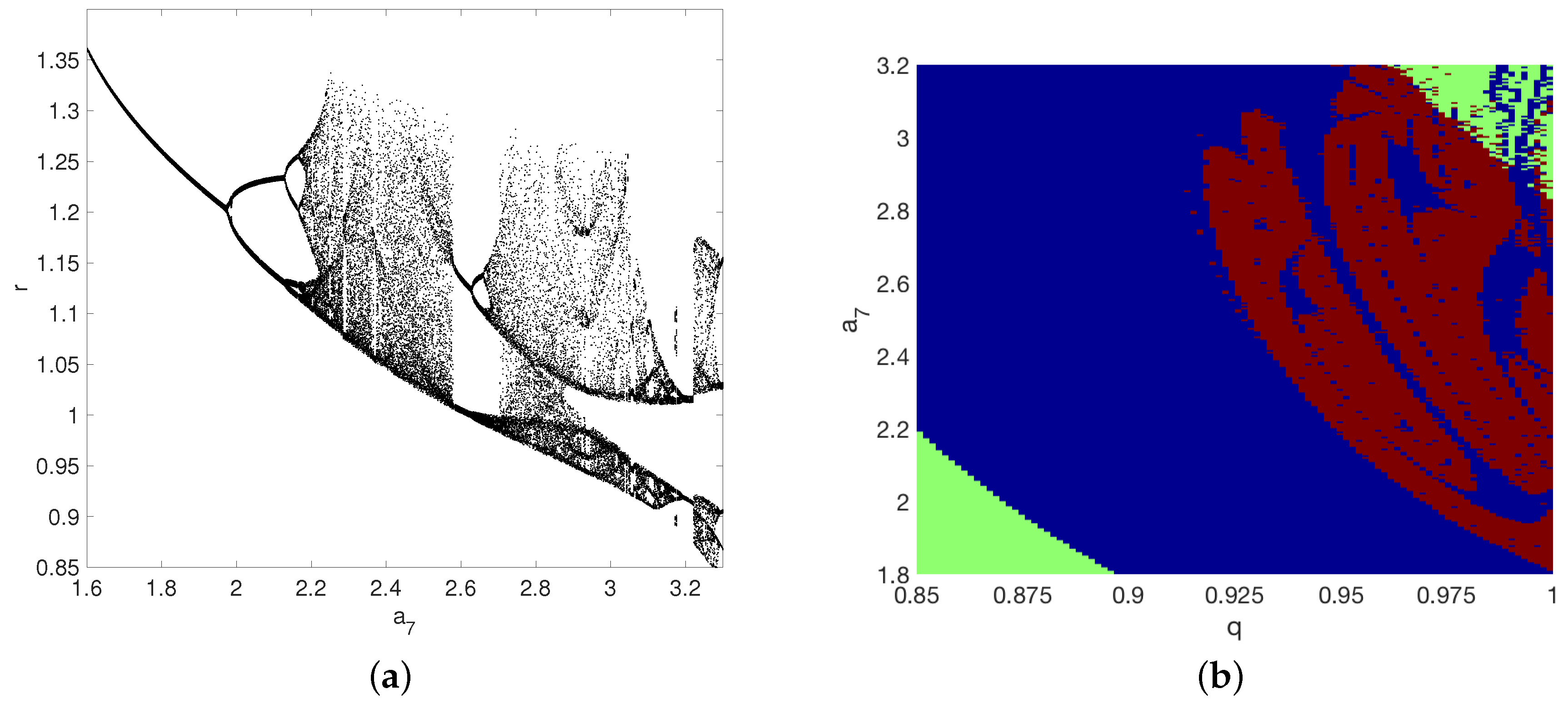
4.3. Type-2 Diabetes Mellitus: Parameter $a_7$ as a Function of Fractional-Order q

The abnormal insulin secretion of the pancreatic $\beta$-cells is commonly related to T2DM or non-insulin-dependent diabetes mellitus, which is known to be a disorder with insulin resistance [80,81,82]. The interconnection among T2DM, insulin resistance, and obesity relies on the $\beta$-cell dysfunction [80,83]. T2DM condition is characterized by the parameter $a_8$ in (5). Figure 8a shows the bifurcation diagram for the parameter $a_8$ with a fractional-order $q=0.98$. The parameter $a_8$ is appropriate to understand the insulin resistance of the human body since it describes the effect of emitted insulin on glucose level [46]. In the bifurcation diagram, that phenomenon is detected when $a_8<0.37$, which is associated with chaotic behavior, as demonstrated by Proposition 2.

Proposition 2.

When $q_1=q_2=q_3\equiv q=0.98$, and $a_1=2.04$, $a_7=2.01$, $a_8=0.27$, $a_{15}=0.3$, the system (5) exhibits a chaotic attractor.

Proof. 

By applying Theorem 3, we can determine the instability measure $\rho$. When $\rho$ is strictly positive, a chaos condition could be established. By selecting $q=0.98$, $a_8=0.27$, and $w=100$ the characteristic polynomial at $E_1=(0.814,1.813,1.320)$ is

$${\lambda }^{294}+2.174{\lambda }^{196}+54.782{\lambda }^{98}-82.2,$$

(25)

with unstable root $\lambda =1.0033$, while at the equilibrium point $E_2=(0.63,0.937,0.879)$ is

$${\lambda }^{294}+1.818{\lambda }^{196}+2.903{\lambda }^{98}+16.537,$$

(26)

with unstable roots ${\lambda }_{1,2}=1.0089\pm 0.0140i$, where the instability measure of the system is $\rho =(\pi /2w)-0.0138>0$. Thus, the system (5) fulfills the essential requirement for getting chaos when $q=0.98$ and $a_1=2.04$, $a_7=2.01$, $a_8=0.27$, $a_{15}=0.3$. □

Additionally, we compute the Lyapunov exponents ${\lambda }_1=0.56$, ${\lambda }_2=0$, ${\lambda }_3=-21.03$. Figure 8b sketches the two-dimensional bifurcation diagram for the T2DM parameter $a_8$ and the fractional-order q. Analogous previous cases, the red areas evolve to chaos, whereas the blue regions converge to a stable behavior (healthy condition). There is a linear fit between the fractional-order and T2DB. The lower the fractional-order, the lower the value for $a_8$, where the T2DM disorder is observed. Besides, for $q<0.97$ the T2DM disappear for $0.25<a_8<0.7$. These results suggest that the T2DM is not presented in the glucose-insulin system (5) for lowers fractional-orders.

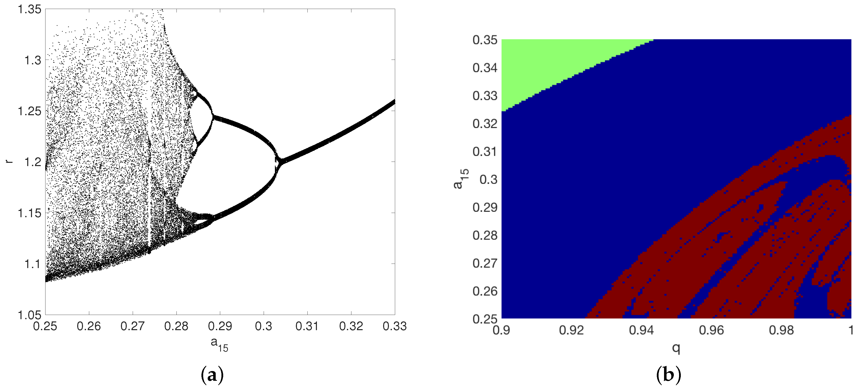
4.4. Type-1 Diabetes Mellitus: Parameter $a_{15}$ as a Function of Fractional-Order q

T1DM is a common autoimmune disease that originates when the pancreatic $\beta$-cells cannot produce insulin at normal levels, and patients will require hormone dosage for their entire life. [84]. The fractional-order system (5) exhibits this condition when the density of $\beta$-cells distinguished by $a_{15}$ reduces and, therefore, the pancreas may not secrete sufficient insulin to stabilize the glucose concentration.

The bifurcation diagram of Equation (5) is shown in Figure 9a when considering $a_{15}$ as critical parameter with $q=0.95$. As can be seen, the system (5) exhibits different types of steady behaviors for specific values of $a_{15}$. However, whether this parameter decreases, the system behaves chaotically, as is demonstrated in Proposition 3.

Proposition 3.

When $q_1=q_2=q_3\equiv q=0.95$ and $a_1=2.04$, $a_7=2.01$, $a_8=0.22$, $a_{15}=0.26$, the system (5) exhibits a chaotic attractor.

Proof. 

By selecting $q=0.95$, $a_{15}=0.26$, and $w=100$, we attain the characteristic polynomial at $E_1=(0.823,1.881,1.366)$ as

$${\lambda }^{285}+2.159{\lambda }^{190}+61.954{\lambda }^{95}-106.369,$$

(27)

being $\lambda =1.0048$ the unstable root. At the equilibrium point $E_2=(0.618,0.883,0.867)$, we obtain

$${\lambda }^{285}+1.765{\lambda }^{190}+1.535{\lambda }^{95}+17.503,$$

(28)

with unstable roots ${\lambda }_{1,2}=1.0091\pm 0.0137i$. Therefore, $\rho =(\pi /2w)-0.0135>0$. In this manner, the proposed system (1) fulfills Theorem 3 for generating a chaotic attractor. □

The Lyapunov exponents when $q=0.95$ and $a_1=2.04$, $a_7=2.01$, $a_8=0.22$, $a_{15}=0.26$ are ${\lambda }_1$ = 1.7733, ${\lambda }_2$ = 0, and ${\lambda }_3$ = −24.3966. Similarly previous case, Figure 9b presents the two-dimensional bifurcation diagram relating $a_{15}$ and the fractional-order q. The green, red, and blue colors denote unbounded, chaotic, and steady-state behaviors, respectively. A healthy behavior, free of T1DM, is found for fractional-orders lowers than $q<0.925$. Those results may imply that lower fractional-orders mitigate the effect of the reduction of population density of $\beta$-cells for T1DM.

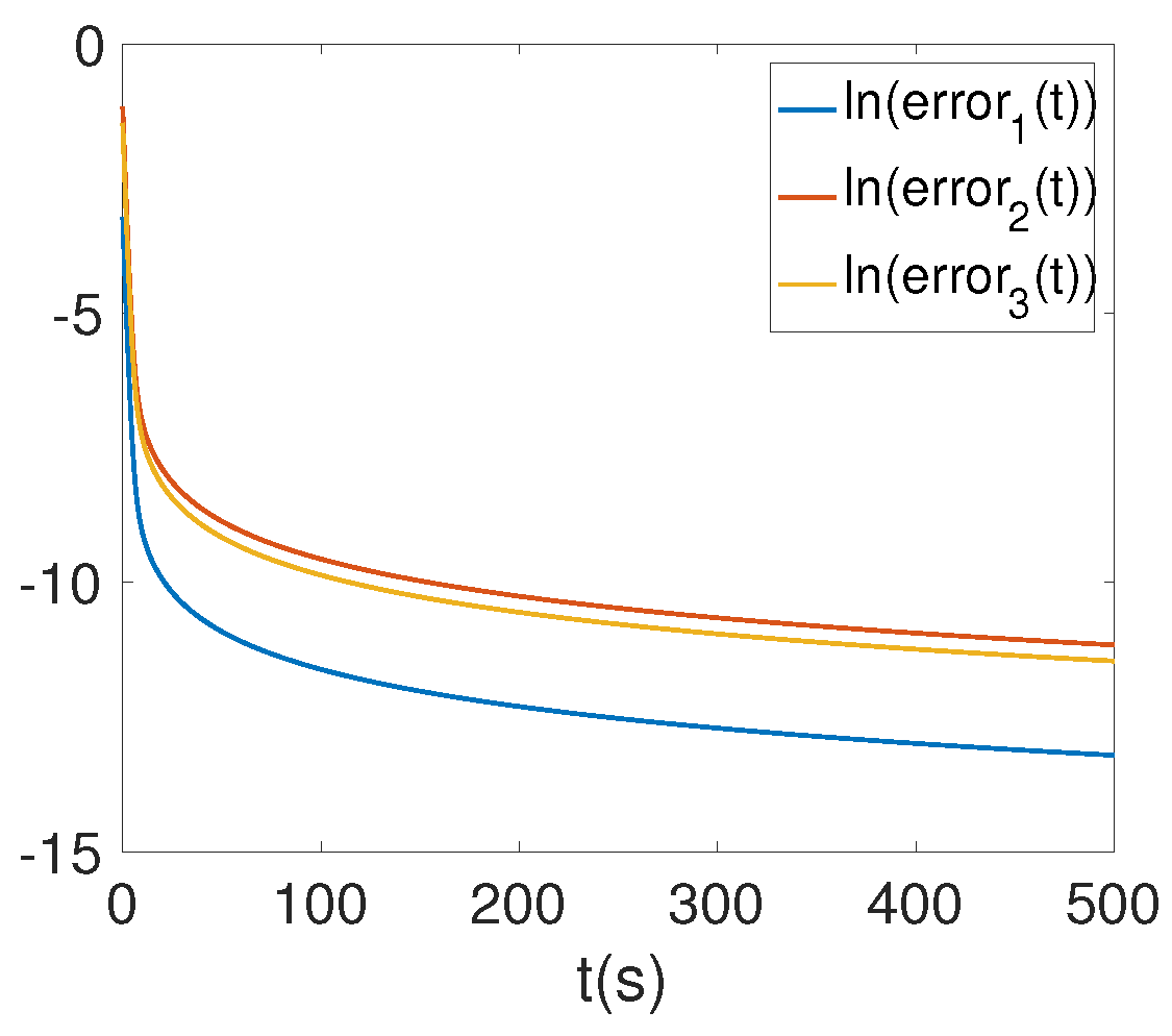
5. Synchronization between Fractional-Order Glucose Insulin Systems

Synchronization is a nonlinear phenomenon that was observed in biological systems; it is seen on isolated cells [15], clusters of cells as in organisms, and even in collective dynamics of populations [25]. Regarding the glucose-insulin system, it has been shown pancreatic $\beta$-cells also present a collective behavior whose synchronization underlies a small-world functional organization [24,25,26]. Thus, the synchronization is crucial to effectuate a pulsatile insulin liberation in cells, which guarantees more substantial hypoglycemic effects. Hence, we study the synchronization between fractional-order glucose-insulin regulatory systems. We expect that the synchronization state converges into a periodic behavior, because it is the typical response in a suband blood glucose concentrations. We define thject with normal metabolic conditions, allowing with this, the synchronization between the insulin e drive and response system, as follows

$$\begin{array}{ccc}\hfill D^{q_1}{x}_1& =& -a_1{x}_1+0.1x_1{y}_1+1.09y_1^2-1.08y_1^3+0.03z_1-0.06z_1^2+a_7{z}_1^3-0.19,\hfill \\ \hfill D^{q_2}{y}_1& =& -a_8{x}_1{y}_1+3.84x_1^2+1.2x_1^3+0.3y_1(1-y_1)-1.37z_1+0.3z_1^2-0.22z_1^3-0.56,\hfill \\ \hfill D^{q_3}{z}_1& =& a_{15}{y}_1-1.35y_1^2+0.5y_1^3+0.42z_1+0.15y_1{z}_1,\hfill \end{array}$$

(29)

and

$$\begin{array}{ccc}\hfill D^{q_1}{x}_2& =& -{\widehat{a}}_1{x}_2+0.1x_2{y}_2+1.09y_2^2-1.08y_2^3+0.03z_2-0.06z_2^2+{\widehat{a}}_7{z}_2^3-0.19+u_1,\hfill \\ \hfill D^{q_2}{y}_2& =& -{\widehat{a}}_8{x}_2{y}_2+3.84x_2^2+1.2x_2^3+0.3y_2(1-y_2)-1.37z_2+0.3z_2^2-0.22z_2^3-0.56+u_2,\hfill \\ \hfill D^{q_3}{z}_2& =& {\widehat{a}}_{15}{y}_2-1.35y_2^2+0.5y_2^3+0.42z_2+0.15y_2{z}_2+u_3,\hfill \end{array}$$

(30)

where $u_1,u_2,u_3$ in (30) represents the unknown control terms, and the error can be defined by

$$\begin{array}{c}\hfill e_1=x_2-x_1,\\ \hfill e_2=y_2-y_1,\\ \hfill e_3=z_2-z_1.\end{array}$$

(31)

To achieve the synchronization, it is essential that the errors $e_i\to 0$ as $t\to \infty$ with $i=1,2,3$. Equation (31), together with (29) and (30), yield the error system

$$\begin{array}{ccc}\hfill D^{q_1}{e}_1& =& -{\widehat{a}}_1{x}_2+0.1x_2{y}_2+1.09y_2^2-1.08y_2^3+0.03z_2-0.06z_2^2+{\widehat{a}}_7{z}_2^3+\hfill \\ & & +a_1{x}_1-0.1x_1{y}_1-1.09y_1^2+1.08y_1^3-0.03z_1+0.06z_1^2-a_7{z}_1^3+u_1,\hfill \\ \hfill D^{q_2}{e}_2& =& -{\widehat{a}}_8{x}_2{y}_2+3.84x_2^2+1.2x_2^3+0.3y_2(1-y_2)-1.37z_2+0.3z_2^2-0.22z_2^3\hfill \\ & & +a_8{x}_1{y}_1-3.84x_1^2-1.2x_1^3-0.3y_1(1-y_1)+1.37z_1-0.3z_1^2+0.22z_1^3+u_2,\hfill \\ \hfill D^{q_3}{e}_3& =& {\widehat{a}}_{15}{y}_2-1.35y_2^2+0.5y_2^3+0.42z_2+0.15y_2{z}_2\hfill \\ & & -a_{15}{y}_1+1.35y_1^2-0.5y_1^3-0.42z_1-0.15y_1{z}_1+u_3.\hfill \end{array}$$

(32)

Let us define the active control functions $u_i$ with $i=1,2,3$

$$\begin{array}{ccc}\hfill u_1& =& V_1+{\widehat{a}}_1{x}_2-0.1x_2{y}_2-1.09y_2^2+1.08y_2^3-0.03z_2+0.06z_2^2-{\widehat{a}}_7{z}_2^3-\hfill \\ & & a_1{x}_1+0.1x_1{y}_1+1.09y_1^2-1.08y_1^3+0.03z_1-0.06z_1^2+a_7{z}_1^3,\hfill \\ \hfill u_2& =& V_2+{\widehat{a}}_8{x}_2{y}_2-3.84x_2^2-1.2x_2^3-0.3y_2(1-y_2)+1.37z_2-0.3z_2^2+0.22z_2^3\hfill \\ & & -a_8{x}_1{y}_1+3.84x_1^2+1.2x_1^3+0.3y_1(1-y_1)-1.37z_1+0.3z_1^2-0.22z_1^3,\hfill \\ \hfill u_3& =& V_3-{\widehat{a}}_{15}{y}_2+1.35y_2^2-0.5y_2^3-0.42z_2-0.15y_2{z}_2\hfill \\ & & +a_{15}{y}_1-1.35y_1^2+0.5y_1^3+0.42z_1+0.15y_1{z}_1,\hfill \end{array}$$

(33)

where the linear functions $V_1,V_2,V_3$ are given by

$$\begin{array}{c}\hfill V_1=-e_1,\\ \hfill V_2=-e_2,\\ \hfill V_3=-e_3.\end{array}$$

(34)

By using (33) and (34), the error system (32) becomes

$$\left[\begin{array}{c}{D}^{q_1}{e}_1\\ D^{q_2}{e}_2\\ D^{q_3}{e}_3\end{array}\right]=\left[\begin{array}{ccc}-1& 0& 0\\ 0& -1& 0\\ 0& 0& -1\end{array}\right]\left[\begin{array}{c}{e}_1\\ e_2\\ e_3\end{array}\right].$$

(35)

The synchronization error vanishes eventually because of the eigenvalues are $-1,-1,-1$ in Equation (35).

The synchronization scenario is as follows. The drive system has a periodic behavior, while the response system is in a chaotic state. We study the Type-1 Diabetes Mellitus (parameter $a_8$), since it is the most common disorder, and affects most world population as well as it is correlated with obesity. For this case, $a_8=0.5$ and ${\widehat{a}}_8=0.27$ for drive and response systems, respectively, while $a_1={\widehat{a}}_1$, $a_7={\widehat{a}}_7$, and $a_{15}={\widehat{a}}_{15}$. The fractional-order are $q_1=q_2=q_3=q=0.95$ in both systems with $x_1\left(0\right)=0.53,y_1\left(0\right)=1.31,z_1\left(0\right)=1.03$ and $x_2\left(0\right)=0.5,y_2\left(0\right)=1.1,z_2\left(0\right)=1.3$, for drive and response systems, respectively. Figure 10a–c show the phase planes between the periodic (free of T1DM) and chaotic (with T1DM) systems. Additionally, the synchronization error by considering (36) is given in Figure 11. Due to the error tends to zero as time evolves, we infer that the proposed control strategy is suitable for forcing the system with the disorder to a state free of T1DM. It is worth noting that the control strategy can be extended to incorporate uncertainties and improve the robustness of the synchronization using other approaches, as shown in [22,85]. From a practical biological point of view, for instance, recent works have employed optical-based control using a light-activated Na+ channel, to attain insulin from $\beta$-cells both in-vitro and vivo [86,87]. Therefore, our results could be useful for future works where the glucose-insulin system could be controlled with an artificial control signal.

$$ln\left(erro{r}_1\left(t\right)\right)=ln{\left(\left[x_2-x_1\right]\right)}^2;ln\left(erro{r}_2\left(t\right)\right)=ln{\left(\left[y_2-y_1\right]\right)}^2;ln\left(erro{r}_3\left(t\right)\right)=ln{\left(\left[z_2-z_1\right]\right)}^2.$$

(36)

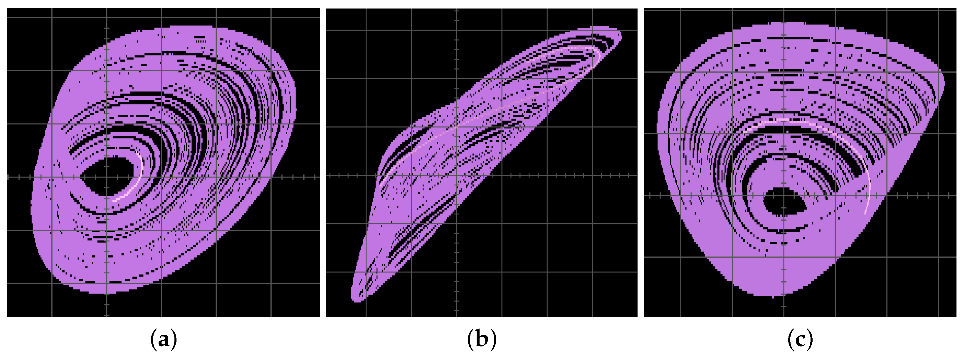
6. Physical Realization of the Fractional-Order Glucose-Insulin System Based on an ARM Processor

As well known, the experimental realization of fractional-order dynamical systems is a hot topic that has been attracting the attention of researchers since it is a path for demonstrating the complex dynamics, including chaos [35,36,37,38,39,44,45]. For fractional-order systems, there three typical approaches for getting electronic circuits: frequency-domain approximation, numerical algorithms, and the Adomian decomposition method [35,36,37,38,39,44,45]. The first-mentioned is not recommended for chaos detection, since it may induce incorrect results [62,63]. On the other hand, the second and latter approaches are good options for physically implementing fractional-order systems in re-programmable digital hardware [44,45]. Therefore, we chose the numerical algorithm approach for programming the ABM method. Subsequently, we select herein the ARM SoC Broadcom BCM2837B0 for the experimental verification of the fractional-order glucose-insulin regulatory system. The SoC contains an ARM core with 64-bit. An SDRAM LPDDR2 with 1GB. The ARM cores are capable of running at up to 1.4 GHz. It’s possible to create an interface by using the GPIO port with a 16-bit monotonic voltage output D/A converter AD569. Figure 12a,b present the block diagram of the working principle and the main instructions of the pseudo-code, respectively.

After initializing the ARM processor, we set the initial values, h, q, $x_0,y_0,z_0$. Because of the negative values of the system (1), a positive integer $\varphi$ is needed to offset the time-series of the state-variables to avoid losing data. In this manner, all computed data are now positive. Next, we multiply the data by a positive integer $\gamma$ to fit them to the DAC resolution of $2^{14}$ bits. Finally, the obtained results visualize in an oscilloscope, as shown in Figure 13 and Figure 14. We analyze the scenario related to hypoglycemia. First, we implement the case where system (1) presents the hypoglycemia condition, as given in Figure 13. As can be seen, the experimental phase portraits are pretty similar to those that are shown in Figure 1. Finally, the case when the fractional-order system (1) is free of hypoglycemia, i.e., an steady-state and, therefore, convergers to a periodic attractor, is given in Figure 14. Similar to the previous case, the experimental results are in good agreement with Figure 4. Subsequently, it indicates that the fractional-order glucose-insulin regulatory system was successfully realized on an ARM digital platform.

7. Conclusions

The dynamical analysis, synchronization, and physical realization of a glucose-insulin regulatory system has been presented by using Caputo’s non-local fractional-order operator. In particular, we studied four common disorders, such as T1DM, T2DM, Hypoglycemia, and Hyperinsulinemia. We found that the fractional-order system switches between a chaotic behavior (a health disorder) and a disorder-free state, not only for the values of systems parameters, but also as a function of the fractional-order, due it adds more degrees of freedom in the model.To understand that insight, we computed two-dimensional bifurcations diagrams, which demonstrated the importance of considering the fractional-order (memory index) for getting a higher approximation of the observed behavior because fractional-order systems describe the whole-time domain in the solution, while the integer-order model is related to the local properties. Additionally, a phenomenon of antimonotonicity was observed in the parameter related to the hyperinsulinemia case. Besides, by applying the straightforward active control method, we showed that stable behavior in the fractional glucose-insulin system under the T1DM condition could be attained when it synchronizes with a disorder-free system. We remark that the synchronization can be extended to the remaining conditions. Finally, the electronics approach-based validation of chaotic and periodic behaviors was shown using an ARM digital platform. The experimental observations were in good agreement with the theoretical findings.

In this manner, the system-of-a-chip circuit designs are the right candidate for exploiting the advantages of the fractional-order models due to their simplicity, programmable characteristics, and portability, therefore increasing the fractional-order-based oncoming applications. As future work, an analysis related to robustness of the synchronization scheme will be developed.

References

1. Röder, P.V.; Wu, B.; Liu, Y.; Han, W. Pancreatic regulation of glucose homeostasis. Exp. Mol. Med. 2016, 48, e219. [Google Scholar] [CrossRef] [PubMed] [Green Version]
2. Puglianiello, A.; Cianfarani, S. Central control of glucose homeostasis. Rev. Diabet. Stud. 2006, 3, 54. [Google Scholar] [CrossRef] [PubMed] [Green Version]
3. Palumbo, P.; Ditlevsen, S.; Bertuzzi, A.; De Gaetano, A. Mathematical modeling of the glucose–insulin system: A review. Math. Biosci. 2013, 244, 69–81. [Google Scholar] [CrossRef] [PubMed]
4. Roglic, G. WHO Global report on diabetes: A summary. Int. J. Noncommun. Dis. 2016, 1, 3. [Google Scholar] [CrossRef]
5. Andrianov, I.; Starushenko, G.; Kvitka, S.; Khajiyeva, L. The Verhulst-Like Equations: Integrable OΔE and ODE with Chaotic Behavior. Symmetry 2019, 11, 1446. [Google Scholar] [CrossRef] [Green Version]
6. Rathee, S. ODE models for the management of diabetes: A review. Int. J. Diabetes Dev. Ctries. 2017, 37, 4–15. [Google Scholar] [CrossRef]
7. Cruz-Duarte, J.M.; Rosales-García, J.J.; Correa-Cely, C.R. Entropy Generation in a Mass-Spring-Damper System Using a Conformable Model. Symmetry 2020, 12, 395. [Google Scholar] [CrossRef] [Green Version]
8. Solís-Pérez, J.E.; Gómez-Aguilar, J.F. Novel Fractional Operators with Three Orders and Power-Law, Exponential Decay and Mittag–Leffler Memories Involving the Truncated M-Derivative. Symmetry 2020, 12, 626. [Google Scholar] [CrossRef] [Green Version]
9. Echenausía-Monroy, J.L.; Huerta-Cuellar, G.; Jaimes-Reátegui, R.; García-López, J.H.; Aboites, V.; Cassal-Quiroga, B.B.; Gilardi-Velázquez, H.E. Multistability Emergence through Fractional-Order- Derivatives in a PWL Multi-Scroll System. Electronics 2020, 9, 880. [Google Scholar] [CrossRef]
10. Danca, M.F. Puu system of fractional order and its chaos suppression. Symmetry 2020, 12, 340. [Google Scholar] [CrossRef] [Green Version]
11. Ionescu, C.; Lopes, A.; Copot, D.; Machado, J.T.; Bates, J. The role of fractional calculus in modeling biological phenomena: A review. Commun. Nonlinear Sci. Numer. Simul. 2017, 51, 141–159. [Google Scholar] [CrossRef]
12. Rihan, F.A. Numerical modeling of fractional-Order biological systems. Abstr. Appl. Anal. 2013, 2013, 816803. [Google Scholar] [CrossRef] [Green Version]
13. Kheiri, H.; Jafari, M. Stability analysis of a fractional order model for the HIV/AIDS epidemic in a patchy environment. J. Comput. Appl. Math. 2019, 346, 323–339. [Google Scholar] [CrossRef]
14. Teka, W.W.; Upadhyay, R.K.; Mondal, A. Spiking and bursting patterns of fractional-order Izhikevich model. Commun. Nonlinear Sci. Numer. Simul. 2018, 56, 161–176. [Google Scholar] [CrossRef]
15. Zambrano-Serrano, E.; Munoz-Pacheco, J.; Gomez-Pavon, L.; Luis-Ramos, A.; Chen, G. Synchronization in a fractional-order model of pancreatic β-cells. Eur. Phys. J. Spec. Top. 2018, 227, 907–919. [Google Scholar] [CrossRef]
16. Bodo, B.; Mvogo, A.; Morfu, S. Fractional dynamical behavior of electrical activity in a model of pancreatic β-cells. Chaos Solitons Fractals 2017, 102, 426–432. [Google Scholar] [CrossRef]
17. Sun, H.; Chen, W.; Wei, H.; Chen, Y. A comparative study of constant-order and variable-order fractional models in characterizing memory property of systems. Eur. Phys. J. Spec. Top. 2011, 193, 185. [Google Scholar] [CrossRef]
18. Saeedian, M.; Khalighi, M.; Azimi-Tafreshi, N.; Jafari, G.; Ausloos, M. Memory effects on epidemic evolution: The susceptible-infected-recovered epidemic model. Phys. Rev. E 2017, 95, 022409. [Google Scholar] [CrossRef] [Green Version]
19. Lundstrom, B.N.; Higgs, M.H.; Spain, W.J.; Fairhall, A.L. Fractional differentiation by neocortical pyramidal neurons. Nat. Neurosci. 2008, 11, 1335. [Google Scholar] [CrossRef]
20. Lifshitz, R.; Cross, M. Response of parametrically driven nonlinear coupled oscillators with application to micromechanical and nanomechanical resonator arrays. Phys. Rev. B 2003, 67, 134302. [Google Scholar] [CrossRef] [Green Version]
21. Bitar, D.; Kacem, N.; Bouhaddi, N. Investigation of modal interactions and their effects on the nonlinear dynamics of a periodic coupled pendulums chain. Int. J. Mech. Sci. 2017, 127, 130–141. [Google Scholar] [CrossRef] [Green Version]
22. Chikhaoui, K.; Bitar, D.; Kacem, N.; Bouhaddi, N. Robustness analysis of the collective nonlinear dynamics of a periodic coupled pendulums chain. Appl. Sci. 2017, 7, 684. [Google Scholar] [CrossRef]
23. Rosenblum, M.G.; Pikovsky, A.S.; Kurths, J. Synchronization approach to analysis of biological systems. Fluct. Noise Lett. 2004, 4, L53–L62. [Google Scholar] [CrossRef] [Green Version]
24. Stožer, A.; Gosak, M.; Dolenšek, J.; Perc, M.; Marhl, M.; Rupnik, M.S.; Korošak, D. Functional connectivity in islets of Langerhans from mouse pancreas tissue slices. PLoS Comput. Biol. 2013, 9, e1002923. [Google Scholar] [CrossRef] [PubMed] [Green Version]
25. Loppini, A.; Cherubini, C.; Filippi, S. On the emergent dynamics and synchronization of β-cells networks in response to space-time varying glucose stimuli. Chaos Solitons Fractals 2018, 109, 269–279. [Google Scholar] [CrossRef]
26. Barua, A.K.; Goel, P. Isles within islets: The lattice origin of small-world networks in pancreatic tissues. Phys. D Nonlinear Phenom. 2016, 315, 49–57. [Google Scholar] [CrossRef]
27. Kotani, K.; Takamasu, K.; Ashkenazy, Y.; Stanley, H.E.; Yamamoto, Y. Model for cardiorespiratory synchronization in humans. Phys. Rev. E 2002, 65, 051923. [Google Scholar] [CrossRef] [Green Version]
28. Bartsch, R.; Kantelhardt, J.W.; Penzel, T.; Havlin, S. Experimental evidence for phase synchronization transitions in the human cardiorespiratory system. Phys. Rev. Lett. 2007, 98, 054102. [Google Scholar] [CrossRef] [Green Version]
29. Satin, L.S.; Butler, P.C.; Ha, J.; Sherman, A.S. Pulsatile insulin secretion, impaired glucose tolerance and type 2 diabetes. Mol. Asp. Med. 2015, 42, 61–77. [Google Scholar] [CrossRef] [Green Version]
30. Ravier, M.A.; Güldenagel, M.; Charollais, A.; Gjinovci, A.; Caille, D.; Söhl, G.; Wollheim, C.B.; Willecke, K.; Henquin, J.C.; Meda, P. Loss of connexin36 channels alters β-cell coupling, islet synchronization of glucose-induced Ca2+ and insulin oscillations, and basal insulin release. Diabetes 2005, 54, 1798–1807. [Google Scholar] [CrossRef] [Green Version]
31. Pecora, L.M.; Carroll, T.L. Synchronization in chaotic systems. Phys. Rev. Lett. 1990, 64, 821. [Google Scholar] [CrossRef]
32. Shukla, M.K.; Sharma, B. Backstepping based stabilization and synchronization of a class of fractional order chaotic systems. Chaos Solitons Fractals 2017, 102, 274–284. [Google Scholar] [CrossRef]
33. Singh, A.K.; Yadav, V.K.; Das, S. Synchronization between fractional order complex chaotic systems with uncertainty. Optik 2017, 133, 98–107. [Google Scholar] [CrossRef]
34. Bai, E.W.; Lonngren, K.E. Synchronization of two Lorenz systems using active control. Chaos Solitons Fractals 1997, 8, 51–58. [Google Scholar] [CrossRef]
35. Shah, D.K.; Chaurasiya, R.B.; Vyawahare, V.A.; Pichhode, K.; Patil, M.D. FPGA implementation of fractional-order chaotic systems. AEU-Int. J. Electron. Commun. 2017, 78, 245–257. [Google Scholar] [CrossRef]
36. Soriano-Sánchez, A.; Posadas-Castillo, C.; Platas-Garza, M.A.; Arellano-Delgado, A. Synchronization and FPGA realization of complex networks with fractional–order Liu chaotic oscillators. Appl. Math. Comput. 2018, 332, 250–262. [Google Scholar]
37. Rajagopal, K.; Akgul, A.; Jafari, S.; Karthikeyan, A.; Koyuncu, I. Chaotic chameleon: Dynamic analyses, circuit implementation, FPGA design and fractional-order form with basic analyses. Chaos Solitons Fractals 2017, 103, 476–487. [Google Scholar] [CrossRef]
38. He, S.; Sun, K.; Wang, H. Complexity analysis and DSP implementation of the fractional-order Lorenz hyperchaotic system. Entropy 2015, 17, 8299–8311. [Google Scholar] [CrossRef] [Green Version]
39. Wang, H.; Sun, K.; He, S. Characteristic analysis and DSP realization of fractional-order simplified Lorenz system based on Adomian decomposition method. Int. J. Bifurc. Chaos 2015, 25, 1550085. [Google Scholar] [CrossRef]
40. Evans, J.R.; Arslan, T. Enhanced image detection on an ARM based embedded system. Des. Autom. Embed. Syst. 2002, 6, 477–487. [Google Scholar] [CrossRef]
41. Tlelo-Cuautle, E.; Rangel-Magdaleno, J.; Pano-Azucena, A.; Obeso-Rodelo, P.; Nuñez-Perez, J.C. FPGA realization of multi-scroll chaotic oscillators. Commun. Nonlinear Sci. Numer. Simul. 2015, 27, 66–80. [Google Scholar] [CrossRef]
42. Chen, H.; He, S.; Azucena, A.D.P.; Yousefpour, A.; Jahanshahi, H.; López, M.A.; Alcaraz, R. A Multistable Chaotic Jerk System with Coexisting and Hidden Attractors: Dynamical and Complexity Analysis, FPGA-Based Realization, and Chaos Stabilization Using a Robust Controller. Symmetry 2020, 12, 569. [Google Scholar] [CrossRef] [Green Version]
43. Munoz-Pacheco, J.M.; García-Chávez, T.; Gonzalez-Diaz, V.R.; de La Fuente-Cortes, G.; del Carmen Gómez-Pavón, L. Two new asymmetric Boolean chaos oscillators with no dependence on incommensurate time-delays and their circuit implementation. Symmetry 2020, 12, 506. [Google Scholar] [CrossRef] [Green Version]
44. Montero-Canela, R.; Zambrano-Serrano, E.; Tamariz-Flores, E.I.; Muñoz-Pacheco, J.M.; Torrealba-Meléndez, R. Fractional chaos based-cryptosystem for generating encryption keys in Ad Hoc networks. Ad Hoc Netw. 2020, 97, 102005. [Google Scholar] [CrossRef]
45. Zambrano-Serrano, E.; Munoz-Pacheco, J.; Campos-Cantón, E. Chaos generation in fractional-order switched systems and its digital implementation. AEU-Int. J. Electron. Commun. 2017, 79, 43–52. [Google Scholar] [CrossRef]
46. Shabestari, P.S.; Panahi, S.; Hatef, B.; Jafari, S.; Sprott, J.C. A new chaotic model for glucose-insulin regulatory system. Chaos Solitons Fractals 2018, 112, 44–51. [Google Scholar] [CrossRef]
47. Letellier, C.; Denis, F.; Aguirre, L.A. What can be learned from a chaotic cancer model? J. Theor. Biol. 2013, 322, 7–16. [Google Scholar] [CrossRef]
48. Jafari, S.; Baghdadi, G.; Golpayegani, S.R.H.; Towhidkhah, F.; Gharibzadeh, S. Is attention deficit hyperactivity disorder a kind of intermittent chaos? J. Neuropsychiatry Clin. Neurosci. 2013, 25, E02. [Google Scholar] [CrossRef]
49. Khajanchi, S.; Perc, M.; Ghosh, D. The influence of time delay in a chaotic cancer model. Chaos Interdiscip. J. Nonlinear Sci. 2018, 28, 103101. [Google Scholar] [CrossRef]
50. Shabestari, P.S.; Rajagopal, K.; Safarbali, B.; Jafari, S.; Duraisamy, P. A Novel Approach to Numerical Modeling of Metabolic System: Investigation of Chaotic Behavior in Diabetes Mellitus. Complexity 2018, 2018, 6815190. [Google Scholar] [CrossRef] [Green Version]
51. Ginoux, J.M.; Ruskeepää, H.; Perc, M.; Naeck, R.; Di Costanzo, V.; Bouchouicha, M.; Fnaiech, F.; Sayadi, M.; Hamdi, T. Is type 1 diabetes a chaotic phenomenon? Chaos Solitons Fractals 2018, 111, 198–205. [Google Scholar] [CrossRef] [Green Version]
52. Rajagopal, K.; Bayani, A.; Jafari, S.; Karthikeyan, A.; Hussain, I. Chaotic dynamics of a fractional order glucose-insulin regulatory system. Front. Inf. Technol. Electron. Eng. 2019, 21, 1108–1118. [Google Scholar] [CrossRef]
53. Ortigueira, M.D.; Machado, J.T. What is a fractional derivative? J. Comput. Phys. 2015, 293, 4–13. [Google Scholar] [CrossRef]
54. Diethelm, K.; Ford, N.J.; Freed, A.D. Detailed error analysis for a fractional Adams method. Numer. Algorithms 2004, 36, 31–52. [Google Scholar] [CrossRef] [Green Version]
55. Diethelm, K.; Ford, N.J. Analysis of fractional differential equations. J. Math. Anal. Appl. 2002, 265, 229–248. [Google Scholar] [CrossRef] [Green Version]
56. Garrappa, R. Numerical solution of fractional differential equations: A survey and a software tutorial. Mathematics 2018, 6, 16. [Google Scholar] [CrossRef] [Green Version]
57. Zambrano-Serrano, E.; Campos-Cantón, E.; Muñoz-Pacheco, J.M. Strange attractors generated by a fractional order switching system and its topological horseshoe. Nonlinear Dyn. 2016, 83, 1629–1641. [Google Scholar] [CrossRef]
58. Li, Y.; Chen, Y.; Podlubny, I. Mittag–Leffler stability of fractional order nonlinear dynamic systems. Automatica 2009, 45, 1965–1969. [Google Scholar] [CrossRef]
59. Petráš, I. Fractional-Order Nonlinear Systems: Modeling, Analysis and Simulation; Springer Science & Business Media: Berlin, Germany, 2011. [Google Scholar]
60. Odibat, Z.; Corson, N.; Aziz-Alaoui, M.; Alsaedi, A. Chaos in fractional order cubic Chua system and synchronization. Int. J. Bifurc. Chaos 2017, 27, 1750161. [Google Scholar] [CrossRef]
61. Ahmed, E.; El-Sayed, A.; El-Saka, H.A. Equilibrium points, stability and numerical solutions of fractional-order predator–prey and rabies models. J. Math. Anal. Appl. 2007, 325, 542–553. [Google Scholar] [CrossRef] [Green Version]
62. Tavazoei, M.; Haeri, M. Unreliability of frequency-domain approximation in recognising chaos in fractional-order systems. IET Signal Process. 2007, 1, 171–181. [Google Scholar] [CrossRef]
63. Tavazoei, M.S.; Haeri, M. A necessary condition for double scroll attractor existence in fractional- order systems. Phys. Lett. A 2007, 367, 102–113. [Google Scholar] [CrossRef]
64. Danca, M.F. Hidden chaotic attractors in fractional-order systems. Nonlinear Dyn. 2017, 89, 577–586. [Google Scholar] [CrossRef] [Green Version]
65. Tavazoei, M.S.; Haeri, M. Chaotic attractors in incommensurate fractional order systems. Phys. D Nonlinear Phenom. 2008, 237, 2628–2637. [Google Scholar] [CrossRef]
66. Ahmed, E.; El-Sayed, A.; El-Saka, H.A. On some Routh–Hurwitz conditions for fractional order differential equations and their applications in Lorenz, Rössler, Chua and Chen systems. Phys. Lett. A 2006, 358, 1–4. [Google Scholar] [CrossRef]
67. Sprott, J.C. Simplest chaotic flows with involutional symmetries. Int. J. Bifurc. Chaos 2014, 24, 1450009. [Google Scholar] [CrossRef]
68. Tourkmani, A.M.; Alharbi, T.J.; Rsheed, A.M.B.; AlRasheed, A.N.; AlBattal, S.M.; Abdelhay, O.; Hassali, M.A.; Alrasheedy, A.A.; Al Harbi, N.G.; Alqahtani, A. Hypoglycemia in Type 2 Diabetes Mellitus patients: A review article. Diabetes Metab. Syndr. Clin. Res. Rev. 2018, 12, 791–794. [Google Scholar] [CrossRef]
69. Wolf, A.; Swift, J.B.; Swinney, H.L.; Vastano, J.A. Determining Lyapunov exponents from a time series. Phys. D Nonlinear Phenom. 1985, 16, 285–317. [Google Scholar] [CrossRef] [Green Version]
70. Effah-Poku, S.; Obeng-Denteh, W.; Dontwi, I. A Study of Chaos in Dynamical Systems. J. Math. 2018, 2018, 1808953. [Google Scholar] [CrossRef] [Green Version]
71. Leonov, G.A.; Kuznetsov, N.V. Time-varying linearization and the Perron effects. Int. J. Bifurc. Chaos 2007, 17, 1079–1107. [Google Scholar] [CrossRef] [Green Version]
72. Lee, Y.; Fluckey, J.D.; Chakraborty, S.; Muthuchamy, M. Hyperglycemia-and hyperinsulinemia-induced insulin resistance causes alterations in cellular bioenergetics and activation of inflammatory signaling in lymphatic muscle. FASEB J. 2017, 31, 2744–2759. [Google Scholar] [CrossRef] [PubMed] [Green Version]
73. Shanik, M.H.; Xu, Y.; Škrha, J.; Dankner, R.; Zick, Y.; Roth, J. Insulin resistance and hyperinsulinemia: Is hyperinsulinemia the cart or the horse? Diabetes Care 2008, 31, S262–S268. [Google Scholar] [CrossRef] [PubMed] [Green Version]
74. Erion, K.A.; Corkey, B.E. Hyperinsulinemia: A cause of obesity? Curr. Obes. Rep. 2017, 6, 178–186. [Google Scholar] [CrossRef] [PubMed] [Green Version]
75. Corkey, B.E. Banting lecture 2011: Hyperinsulinemia: Cause or consequence? Diabetes 2012, 61, 4–13. [Google Scholar] [CrossRef] [PubMed] [Green Version]
76. Glaser, B. Type 2 diabetes: Hypoinsulinism, hyperinsulinism, or both? PLoS Med. 2007, 4, e148. [Google Scholar] [CrossRef] [PubMed] [Green Version]
77. Dawson, S.P.; Grebogi, C.; Yorke, J.A.; Kan, I.; Koçak, H. Antimonotonicity: Inevitable reversals of period-doubling cascades. Phys. Lett. A 1992, 162, 249–254. [Google Scholar] [CrossRef]
78. Kengne, J.; Jafari, S.; Njitacke, Z.; Khanian, M.Y.A.; Cheukem, A. Dynamic analysis and electronic circuit implementation of a novel 3D autonomous system without linear terms. Commun. Nonlinear Sci. Numer. Simul. 2017, 52, 62–76. [Google Scholar] [CrossRef]
79. Signing, V.F.; Kengne, J.; Pone, J.M. Antimonotonicity, chaos, quasi-periodicity and coexistence of hidden attractors in a new simple 4-D chaotic system with hyperbolic cosine nonlinearity. Chaos Solitons Fractals 2019, 118, 187–198. [Google Scholar] [CrossRef]
80. Pandey, A.; Chawla, S.; Guchhait, P. Type-2 diabetes: Current understanding and future perspectives. IUBMB Life 2015, 67, 506–513. [Google Scholar] [CrossRef]
81. Bhattacharya, S.; Dey, D.; Roy, S.S. Molecular mechanism of insulin resistance. J. Biosci. 2007, 32, 405–413. [Google Scholar] [CrossRef] [Green Version]
82. Quan, W.; Jo, E.K.; Lee, M.S. Role of pancreatic β-cell death and inflammation in diabetes. Diabetes Obes. Metab. 2013, 15, 141–151. [Google Scholar] [CrossRef] [PubMed]
83. Weng, J.; Li, Y.; Xu, W.; Shi, L.; Zhang, Q.; Zhu, D.; Hu, Y.; Zhou, Z.; Yan, X.; Tian, H.; et al. Effect of intensive insulin therapy on β-cell function and glycaemic control in patients with newly diagnosed type 2 diabetes: A multicentre randomised parallel-group trial. Lancet 2008, 371, 1753–1760. [Google Scholar] [CrossRef]
84. Pearson, J.A.; Agriantonis, A.; Wong, F.S.; Wen, L. Modulation of the immune system by the gut microbiota in the development of type 1 diabetes. Hum. Vaccines Immunother. 2018, 14, 2580–2596. [Google Scholar] [CrossRef] [PubMed] [Green Version]
85. Jahanshahi, H.; Yousefpour, A.; Munoz-Pacheco, J.M.; Kacar, S.; Pham, V.T.; Alsaadi, F.E. A new fractional-order hyperchaotic memristor oscillator: Dynamic analysis, robust adaptive synchronization, and its application to voice encryption. Appl. Math. Comput. 2020, 383, 125310. [Google Scholar] [CrossRef]
86. Nasteska, D.; Hodson, D.J. The role of beta cell heterogeneity in islet function and insulin release. J. Mol. Endocrinol. 2018, 61, R43–R60. [Google Scholar] [CrossRef] [Green Version]
87. Reinbothe, T.M.; Safi, F.; Axelsson, A.S.; Mollet, I.G.; Rosengren, A.H. Optogenetic control of insulin secretion in intact pancreatic islets with β-cell-specific expression of Channelrhodopsin-2. Islets 2014, 6, e28095. [Google Scholar] [CrossRef] [Green Version]
Figure 1. Eigenvalues of the system (5) in the complex plane. (a) eigenvalues for equilibria E 1 , (b) eigenvalues for equilibria E 2 .
Symmetry 12 01395 g001
Figure 2. Chaotic attractor of the fractional-order glucose-insulin model (5) for fractional-orders q = 0.9 , a 1 = 1.3 , a 7 = 2.01 , a 8 = 0.22 , a 15 = 0.3 , ( x 0 , y 0 , z 0 ) = ( 0.5 , 1.2 , 1 ) , and integration step-size h = 0.01 . (a) x y phase plane, (b) x z phase plane, (c) y z phase plane.
Symmetry 12 01395 g002
Figure 3. (a) Bifurcation diagram varying the hypoglycemia parameter a 1 and setting q = 0.9 , and (b) its Lyapunov exponent spectrum when a 1 = 1.3 .
Symmetry 12 01395 g003
Figure 4. (a) Two-dimensional bifurcation diagram for the hypoglycemia parameter a 1 and fractional-order q, where green region stands for unbounded behavior, red for chaotic behavior, and blue regions lead to healthy (periodic) behavior. (b) Basin of attraction on the x ( 0 ) y ( 0 ) plane with z ( 0 ) = 1 , q = 0.9 , and a 1 = 1.3 showing the chaotic behavior. The initial conditions marked in the yellow color lead into a bounded chaotic attractor, whereas the initial conditions in blue region converge into unbounded behavior.
Symmetry 12 01395 g004
Figure 5. Stable behavior of the fractional-order system (5) considering q = 0.9 , a 1 = 1.55 , and initial conditions ( x 0 , y 0 , z 0 ) = ( 0.5 , 1.2 , 1 ) , with a integration step-size h = 0.01 . (a) x y phase plane, (b) x z phase plane, (c) y z phase plane.
Symmetry 12 01395 g005
Figure 6. Lyapunov spectrum of (5): a 1 = 1.55 and q = 0.9 .
Symmetry 12 01395 g006
Figure 7. (a) Bifurcation diagram varying the hyperinsulinemia parameter a 7 and setting q = 0.95 and (b) Two-dimensional bifurcation diagram for a 7 and fractional-order q where the unbounded behavior is represented by the green regions; chaotic behavior is denoted by red regions, and the healthy behavior (free of hyperinsulinemia) is given by the blue regions.
Symmetry 12 01395 g007
Figure 8. (a) Bifurcation diagram varying the T2DM parameter a 8 and setting q = 0.98 and (b) Two-dimensional bifurcation diagram for a 8 and fractional-order q, the chaotic behavior is denoted by red regions, and the periodic behavior (healthy behavior) is given by the blue regions.
Symmetry 12 01395 g008
Figure 9. (a) Bifurcation diagram varying the T1DM parameter a 15 and setting q = 0.95 , and (b) Two-dimensional bifurcation diagram for a 15 and fractional-order q. The unbounded behavior is represented by the green regions; chaotic behavior is denoted by red regions, and the periodic behavior (healthy behavior) is given by the blue regions.
Symmetry 12 01395 g009
Figure 10. Synchronization planes for the fractional-order glucose-insulin systems (29) and (30) with a 8 = 0.5 , a ^ 8 = 0.27 , and q = 0.95 , respectively. (a) x 1 x 2 phase plane, (b) y 1 y 2 phase plane, (c) z 1 z 2 phase plane.
Symmetry 12 01395 g010
Figure 11. Synchronization error between the fractional-order glucose-insulin systems (29) and (30) when a 8 = 0.5 , a ^ 8 = 0.27 , q = 0.95 , and ( x 1 , y 1 , z 1 , x 2 , y 2 , z 2 ) = ( 0.53 , 1.31 , 1.03 , 0.49 , 1 , 0.8 ) , respectively.
Symmetry 12 01395 g011
Figure 12. (a) Simplified diagram of the implementation of the fractional-order glucose-insulin regulatory system (1), and (b) the main steps of the proposed algorithm for implementing it on an ARM digital platform.
Symmetry 12 01395 g012
Figure 13. Experimental phase portraits of the fractional-order glucose-insulin regulatory system (1) showing hypoglycemia (chaos behavior) with h = 0.01 , a 1 = 1.3 , a 7 = 2.01 , a 8 = 0.22 , a 15 = 0.3 , q 1 = q 2 = q 3 = 0.9 and ( x 0 , y 0 , z 0 ) = ( 0.5 , 1.2 , 1 ) . (a) x y plane, (b) x z plane, (c) y z plane.
Symmetry 12 01395 g013
Figure 14. Experimental phase portraits of the fractional-order glucose-insulin regulatory system (1) depicting a steady-state free of hypoglycemia with h = 0.01 , a 1 = 1.55 , a 7 = 2.01 , a 8 = 0.22 , a 15 = 0.3 , q 1 = q 2 = q 3 = 0.9 and ( x 0 , y 0 , z 0 ) = ( 0.5 , 1.2 , 1 ) .(a) x y plane, (b) x z plane, (c) y z plane.
Symmetry 12 01395 g014