On Approximate Aesthetic Curves

Abstract

Symmetry plays an essential role for generating aesthetic forms. The curve is the basic element used by designers to obtain aesthetic forms. A curve with a linear logarithmic curvature graph gradient is called aesthetic curve. The aesthetic value of a curve increases when its gradient is close to a straight line. We introduce the notions of approximate aesthetic curves and approximate neutral curves and obtain estimations between the curvature of an approximate aesthetic/neutral curve and an aesthetic curve.

1. Introduction

The curve is the basic design element used to obtain shapes and silhouettes of industrial products. This is why designers try to make it aesthetic in order to improve the quality of the shape design. The aesthetic aspect of a curve is one of the most studied topics [1,2]. Farin considers that one of the main aspects that must be used in the evaluation of an aesthetic curve is its curvature distribution [3,4]. If the changes of the curvature are constant, i.e., the second derivative of the curve is monotonic, then the curve is beautiful [4,5,6]. Among them, a family of curves called the log-aesthetic curves has been deeply investigated with respect to the relation between designers′ visual languages and mathematical properties; see for example [7]. The Logarithmic Distribution Diagram of Curvature (LDDC) was used to analyze the characteristics of planar curves with monotonic curvature by Harada et al. in [8]. LDDC describes the relation between the length frequencies of a segmented curve with respect to its radius of curvature plotted in log-log coordinate system. The aesthetic value of a curve for automobile design can be identified based on these graphs [6,8]. In 2003, Kanaya et al. [9] proposed the generation of Logarithmic Curvature Histogram (LCH) to substitute LDDC; see also [10,11]. Gobithaasan et al. [8] proposed the formula of the Logarithmic Curvature Graph’s (LCG) gradient to define an aesthetic curve: a curve with a constant or a linear LCG gradient is called aesthetic curve. Moreover, he obtained a classification of aesthetic curves taking into consideration the sign of the gradient. In [12], the authors obtain a relation for the curvature if the gradient of the curve is linear. New aesthetic standards based on the Golden Ratio and its generalization have been proposed in [1,2].

Several research studies have focused on determining the aesthetics of an object and on identifying how certain object features evoke feelings during their perception. Despite the large number of definitions and approaches, there is not a generally valid model for determining the aesthetic value of an object because “the visual perceptions are accompanied by a certain intuitive feeling of value” called aesthetic feeling [13,14]. Since people’s perceptions of aesthetics are not necessarily objective, we propose two new notions in this paper, namely approximate aesthetic curve and approximate neutral curves, and we study their relation to an aesthetic curve. For each class of curves, the paper includes a definition, a characterization theorem as well as illustrative applications. The notion of approximate aesthetic curve, corresponding to an approximate solution of an equation, is connected to the notion of Ulam Stability of that equation. An equation is called Ulam stable if for every approximate solution of it there exists an exact solution of the equation near it.

2. Aesthetic Curves

Let $\left(C\right)$ be an arc-length $s$ parameterized curve defined by the equations:

$$r\left(s\right)=\left(x\left(s\right),y\left(s\right)\right),0\le s\le S,$$

(1)

where $S$ is the total length of the curve and $r$ is a point of coordinates $x$,$y$ on $\left(C\right)$.

The Logarithmic Curvature Graph (LCG) gradient is given by the relation:

$$\lambda (s)=\frac{k^{″}\left(s\right)k\left(s\right)}{{\left(k^{\prime }\left(s\right)\right)}^2}-1,0\le s\le S,$$

(2)

where $k$ is the curvature of $\left(C\right)$ and $k$ is a nonconstant function (see [7]). The notion of aesthetic curve is defined in [8] as follows:

Definition 1.

[8]. A curve is said to be an aesthetic curve if its LCG gradient is either constant or the gradient is represented by a straight line with a nonzero slope.

A classification of aesthetic curves is given below.

Definition 2.

[8]. An aesthetic curve is called:

• Convergent: if the LCG gradient is positive;
• Divergent: if the LCG gradient is negative;
• Neutral: if the LCG gradient is zero.

In the next theorem, we give a characterization of convergent, divergent, and neutral curves and obtain their representation.

Theorem 1.

Let$\left(C\right)$be a curve given by (1). Then:

• $\left(C\right)$is convergent if and only if$\left|k\right|$is strictly decreasing;
• $\left(C\right)$is divergent if and only if$\left|k\right|$is strictly increasing;
• $\left(C\right)$is neutral if and only if$k\left(s\right)=c_2{e}^{c_{1}s},0\le s\le S$, and c₁, c₂ are real constants.

Proof. 

1. $\left(C\right)$ is convergent $\iff \lambda \left(s\right)>0,0\le s\le S$, which is equivalent to:

$$\frac{k^{″}\left(s\right)k\left(s\right)}{{\left(k^{\prime }\right(s\left)\right)}^2}-1>0,0\le s\le S.$$

(3)

Let $z$ be defined by $z\left(s\right)=\frac{k\left(s\right)}{k^{\prime }\left(s\right)},s\in \left[0,S\right]$. Then $z^{\prime }\left(s\right)=\frac{{\left(k^{\prime }\left(s\right)\right)}^2-k^{″}\left(s\right)k\left(s\right)}{{\left(k^{\prime }\left(s\right)\right)}^2}=-\lambda \left(s\right)$,$0 \le s\le S , s\in \left[0,S\right]$. Then the relation (3) becomes $z^{\prime }\left(s\right)<0$ or $\frac{k^{\prime }\left(s\right)}{k\left(s\right)}<0,s\in \left[0,S\right]$, which is equivalent to $\left(\log \left|k\left(s\right)\right|\right){}^{\prime }<0,s\in \left[0,S\right]$. Therefore $\log \left|k\right|$ is a strictly decreasing function. We conclude that $\left|k\right|$ is a strictly decreasing function since log is strictly increasing.

2. Similarly, we get, for divergent curves, $\frac{k^{\prime }\left(s\right)}{k\left(s\right)}>0,s\in \left[0,S\right]$. So $\left|k\right|$ is an increasing function.

3. If $\left(C\right)$ is a neutral curve, then $\lambda \left(s\right)=0$ or $z^{\prime }\left(s\right)=0,s\in \left[0,S\right]$ and integrating with respect to $s$ it follows:

$$k\left(s\right)=c_2{e}^{c_{1}s};0\le s\le S$$

where $c_1,c_2\in \mathbb{R}$ are arbitrary constants.

The representations of the curves can be obtained from the following relation (see [8]):

$$r\left(s\right)=\left(x\left(0\right)+{\displaystyle \underset{0}{\overset{S}{\int }}\cos \left(\theta \left(0\right)+{\displaystyle \underset{0}{\overset{t}{\int }}k\left(u\right)du}\right)}dt,\mathrm{y}\left(0\right)+{\displaystyle \underset{0}{\overset{S}{\int }}\sin \left(\theta \left(0\right)+{\displaystyle \underset{0}{\overset{t}{\int }}k\left(u\right)du}\right)}dt\right)$$

(4)

where $\theta \left(s\right),0\le s\le S$ is the measure in radians of the angle from the positive axis $x$ to the unit tangent vector to the curve. □

3. Approximate Neutral Curves

In [8] is defined the notion of an aesthetic curve as a curve with the LCG gradient constant or a straight line. The authors also mention that the aesthetic value of the curve increases when the LCG gradient approximates to a straight line, and, in particular, for neutral curves to zero. In what follows, we propose a definition for measuring the aesthetic value for a neutral curve in the sense mentioned above.

Definition 3.

Let$\epsilon >0$. We say that a curve$\left(C\right)$:$r\left(s\right)=\left(x\left(s\right),y\left(s\right)\right),0\le s\le S,$is$\epsilon -$neutral curve if its LCG gradient$\lambda$satisfies the relation:

$$\left|\lambda \left(s\right)\right|\le \epsilon ,$$

(5)

for all$s,\hspace{0.17em}0\le s\le S$.

A curve satisfying (5) for some positive $\epsilon$ is called approximate neutral curve.

For an $\epsilon -$neutral curve we will give an estimation of its curvature. Since in the definition of the gradient we suppose that $k^{\prime }\left(s\right)\ne 0$ for all $s,\hspace{0.17em}0\le s\le S$, we deduce that $k^{\prime }\left(s\right)>0$ or $k^{\prime }\left(s\right)<0$ on the interval $\left[0,S\right]$. So, according to Theorem 2, the curve $\left(C\right)$ is either convergent or divergent.

Theorem 2.

Suppose that$\left(C\right)$is an$\epsilon -$neutral convergent curve given by (1). Then its curvature satisfies the following relation

$$\left|k\left(s\right)\right|\le \left|k\left(0\right)\right|{\left|1-\frac{k^{\prime }\left(0\right)}{k\left(0\right)}\epsilon s\right|}^{-\frac{1}{\epsilon }},0\le s\le S.$$

(6)

Proof. 

The curve $\left(C\right)$ satisfies the relation $0<\lambda \left(s\right)\le \epsilon$, which is equivalent to

$$0\le \frac{k^{″}\left(s\right)k\left(s\right)}{{\left(k^{\prime }\left(s\right)\right)}^2}-1\le \epsilon ,0\le s\le S.$$

(7)

Let $z\left(s\right)=\frac{k\left(s\right)}{k^{\prime }\left(s\right)},s\in \left[0,S\right]$. Then (7) becomes $0\ge z^{\prime }\left(s\right)\ge -\epsilon ,0\le s\le S$, which leads to

$$0\ge z\left(s\right)-z\left(0\right)\ge -\epsilon s,0\le s\le S.$$

It follows $0\ge \frac{k\left(s\right)}{k^{\prime }\left(s\right)}\ge z\left(0\right)-\epsilon s$ or $\frac{k^{\prime }\left(s\right)}{k\left(s\right)}\le \frac{1}{z\left(0\right)-\epsilon s},0\le s\le S.$ □

Integrating the previous relation on $\left[0,s\right]$ and taking account that $z\left(0\right)<0$ we get

$$\log \left|k\left(s\right)\right|-\log \left|k\left(0\right)\right|\le -\frac{1}{\epsilon }\log \left|1-\frac{k^{\prime }\left(0\right)}{k\left(0\right)}\epsilon s\right|$$

or

$$\left|k\left(s\right)\right|\le \left|k\left(0\right)\right|{\left|1-\frac{k^{\prime }\left(0\right)}{k\left(0\right)}\epsilon s\right|}^{-\frac{1}{\epsilon }},0\le s\le S.$$

Remark 1.

$\underset{\begin{array}{l}\epsilon \to 0\\ \epsilon >0\end{array}}{\overset{}{\lim }}{\left(1-\frac{k^{\prime }\left(0\right)}{k\left(0\right)}\epsilon s\right)}^{-\frac{1}{\epsilon }}=\underset{\begin{array}{l}\epsilon \to 0\\ \epsilon >0\end{array}}{\overset{}{\lim }}{e}^{-\frac{k^{\prime }\left(0\right)}{k\left(0\right)}\epsilon s\left(-\frac{1}{\epsilon }\right)}=e^{\frac{k^{\prime }\left(0\right)}{k\left(0\right)}s}=e^{c_{1}s}$.

An analogous result holds for convergent curves.

Theorem 3.

Suppose that$\left(C\right)$is an$\epsilon -$neutral divergent curve given by (1) with$k\left(0\right)\ne 0$. Then its curvature satisfies the following estimation:

$$\left|k\left(s\right)\right|\ge \left|k\left(0\right)\right|{\left(1+\frac{k^{\prime }\left(0\right)}{k\left(0\right)}\epsilon s\right)}^{\frac{1}{\epsilon }},0\le s\le S.$$

(8)

Proof. 

The gradient of $\left(C\right)$ satisfies the relation:

$$-\epsilon \le \lambda \left(s\right)<0,0\le s\le S$$

and the function $z$ defined in the proof of the Theorem 3 satisfies the double inequality:

$$0<z\left(s\right)\le z\left(0\right)+\epsilon s,0\le s\le S.$$

The curvature $k$ fulfills the relation

$$\frac{k^{\prime }\left(s\right)}{k\left(s\right)}\ge \frac{1}{z\left(0\right)+\epsilon s}$$

which leads to

$$\log \left|k\left(s\right)\right|+\log \left|k\left(0\right)\right|\ge \frac{1}{\epsilon }\log \left(\frac{z\left(0\right)+\epsilon s}{z\left(0\right)}\right)$$

or

$$\left|k\left(s\right)\right|\ge \left|k\left(0\right)\right|{\left(1+\frac{k^{\prime }\left(0\right)}{k\left(0\right)}\epsilon s\right)}^{\frac{1}{\epsilon }},0\le s\le S.$$

The theorem is proved. □

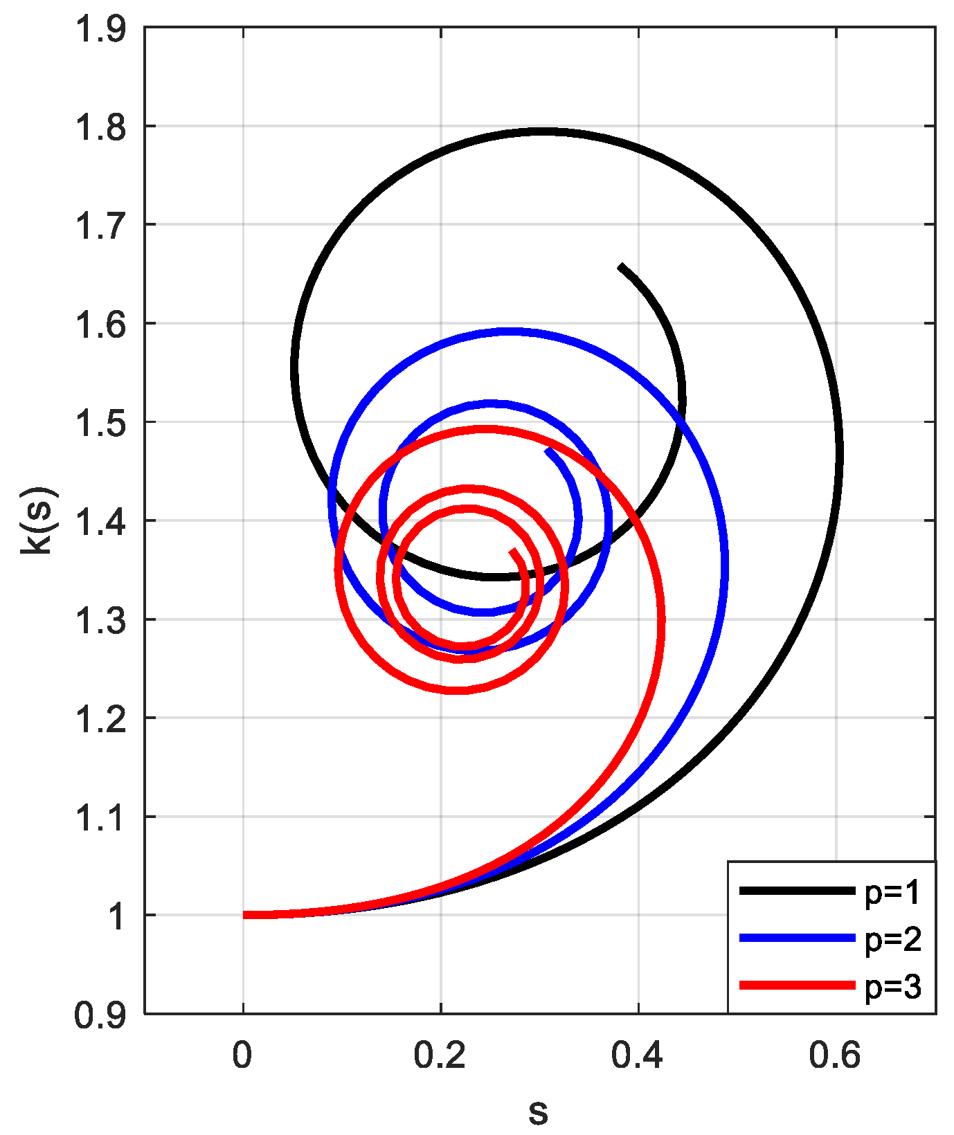
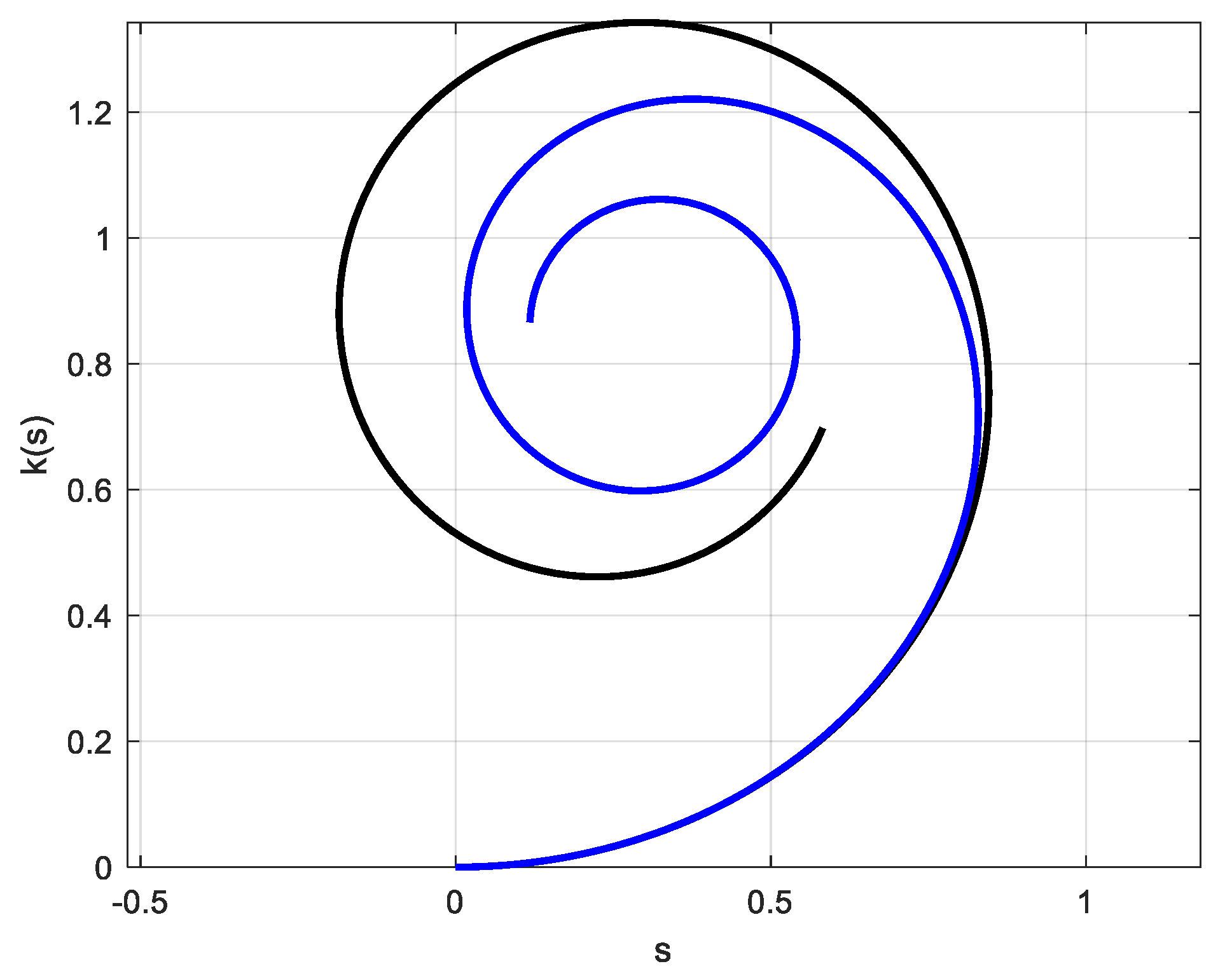
Application 1.

Let$\left(C\right)$be an$\epsilon -$neutral convergent curve with$\epsilon =1,k\left(0\right)=1,k^{\prime }\left(0\right)=-1$. Then, from Theorem 3 we obtain:

$$0<k\left(s\right)\le \frac{1}{1+s},0\le s\le S.$$

So, every curve with $k_p\left(s\right)=\frac{1}{1+ps},p\in \left\{1,2,3\right\}$ satisfies the previous inequality and the corresponding neutral curve has the curvature $k\left(s\right)=e^{-s},0\le s\le S.$

Taking for the representation of the approximate neutral curves $x\left(0\right)=0,y\left(0\right)=1,\theta \left(0\right)=0$ we obtain a family of logarithmic spirals (Figure 1).

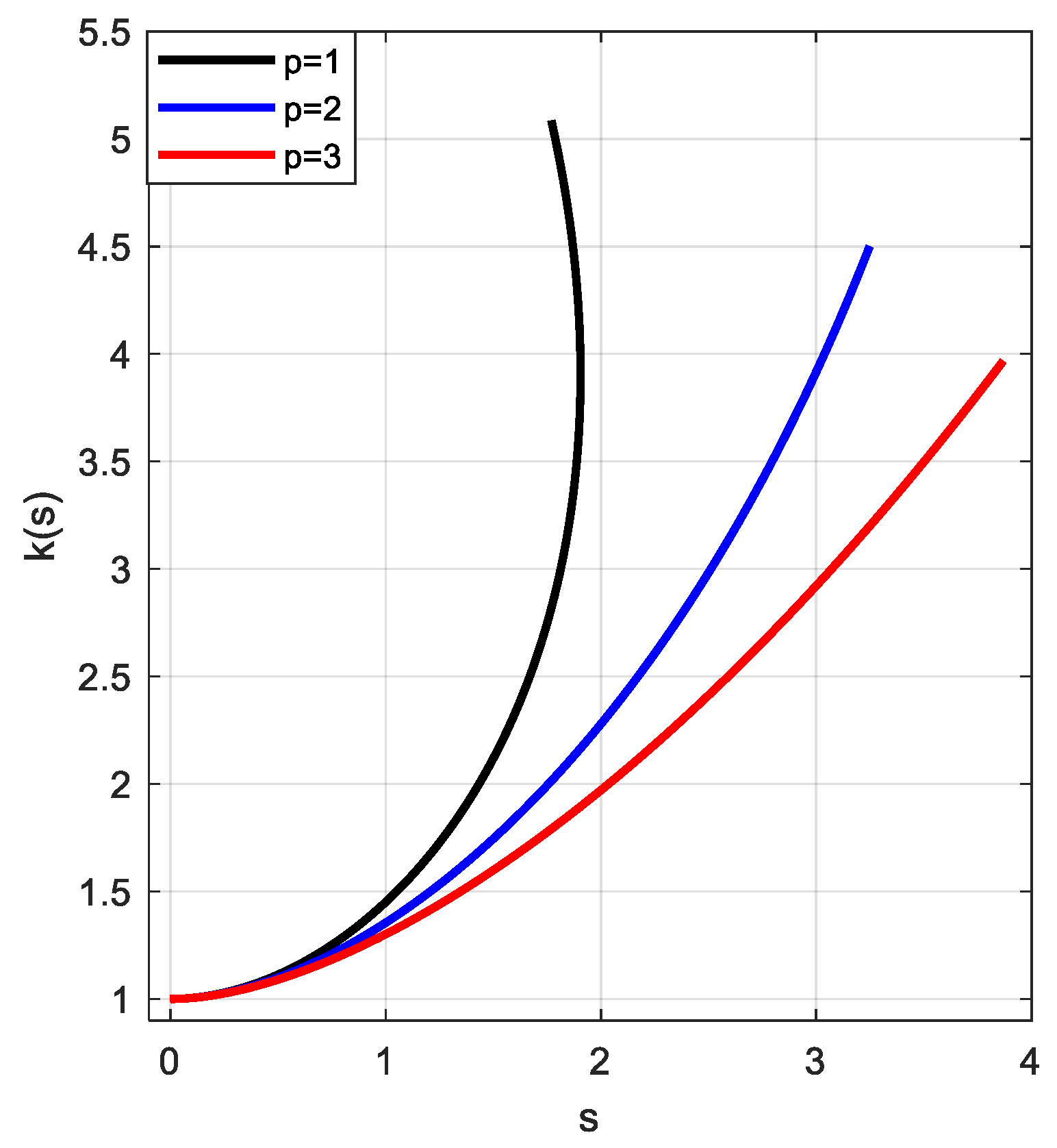
Application 2.

For$\epsilon ={10}^{-1},k\left(0\right)=1$and$k^{\prime }\left(0\right)=-1$we have$k\left(s\right)\le {\left(1+\frac{s}{10}\right)}^{-10}.$

Taking account of the well-known inequality $1+x\le e^x,\forall x\in ℝ$, it can be easily shown that $e^{-s}\le {\left(1+\frac{s}{10}\right)}^{-10}.$

If we consider $x\left(0\right)=0,y\left(0\right)=1,\theta \left(0\right)=-\frac{\pi }{4},k_p\left(s\right)={\left(1+\frac{s}{10}\right)}^p,p\in \left\{-10,-20,-30\right\},$ then $r\left(s\right)$ is easily computed using Legendre–Gauss quadrature for each case and the graphical representations of the curves are given in Figure 2 together with the plot of the curve obtained for $k\left(s\right)=e^{-s}.$ The mentioned numerical integration method has been used for the computation of all definite integrals within this paper.

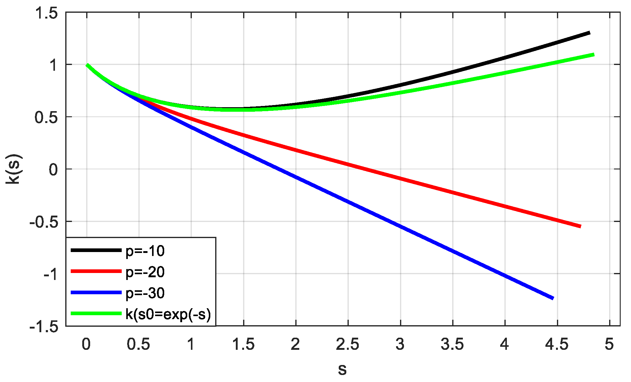
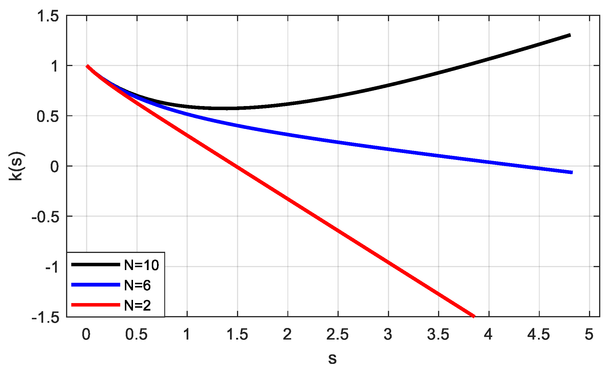
If we consider $x\left(0\right)=0,y\left(0\right)=1,\theta \left(0\right)=-\frac{\pi }{4},k_N\left(s\right)={\left(1+\frac{s}{N}\right)}^{-10},N\in \left\{2,6,10\right\}$ then $r\left(s\right)$ is easily computed for each case and the graphical representations of the curves are given in Figure 3.

Application 3.

Let$\left(C\right)$be an$\epsilon -$neutral divergent curve with$\epsilon =1,k\left(0\right)=k^{\prime }\left(0\right)=1$. Then from Theorem 3 we obtain$k\left(s\right)>1+s,0\le s\le S.$

So, every curve with $k_p\left(s\right)=1+ps,p\in \left\{1,2,3\right\}$ satisfies the inequality above. Taking for the representation of the approximate neutral curves $x\left(0\right)=0,y\left(0\right)=1$ we obtain a family of Euler spirals (Figure 4). The corresponding neutral curve has the curvature $k\left(s\right)=e^s,0\le s\le S.$

4. Approximate Aesthetic Curves

Similarly to $\epsilon -$neutral curves we define the notion of $\epsilon -$aesthetic curve in spirit of Definition 3.

Definition 4.

Let$\epsilon \ge 0$. A curve$\left(C\right)$of LCG gradient$\lambda$is called$\epsilon -$aesthetic curve if there exist real numbers a, b such that:

$$\left|\lambda \left(s\right)-as-b\right|\le \epsilon ,0\le s\le S.$$

(9)

Clearly if $\epsilon =0$ then $\lambda \left(s\right)=as+b$ for all $s\in \left[0,S\right].$ Therefore, $\left(C\right)$ is an aesthetic curve. If $a=b=0$ then we get the notion of $\epsilon -$neutral curve studied in Section 3 of this paper. A curve that is $\epsilon -$aesthetic for some $\epsilon \ge 0$ is called approximate aesthetic curve.

Our goal is to obtain an estimation of the curvature for an approximate aesthetic curve. For this we need some auxiliary results.

Theorem 4.

Let$\left(C\right)$be a curve of gradient$\lambda$with$k\left(0\right)\ne 0$. Then its curvature$k$is given by the relation:

$$k\left(s\right)=C_2{e}^{{\displaystyle \underset{0}{\overset{s}{\int }}\frac{1}{C_1-{\displaystyle {\int }_0^u\lambda \left(t\right)dt}}du}},s\in \left[0,S\right],$$

(10)

where C₁, C₂ are real constants. Moreover,$C_1=\frac{k\left(0\right)}{k^{\prime }\left(0\right)},C_2=k\left(0\right).$

Proof. 

The curvature $k\left(s\right)$ is the solution of the differential equation

$$\frac{k^{″}\left(s\right)k\left(s\right)}{{\left(k^{\prime }\left(s\right)\right)}^2}-1=\lambda \left(s\right),s\in \left[0,S\right].$$

(11)

The function $z,z\left(s\right)=\frac{k\left(s\right)}{k^{\prime }\left(s\right)},s\in \left[0,S\right],$ satisfies the equation $-z^{\prime }\left(s\right)=\lambda \left(s\right),s\in \left[0,S\right].$ So $z\left(s\right)=-{\displaystyle \underset{0}{\overset{s}{\int }}\lambda \left(t\right)dt}+C_1,C_1=z\left(0\right).$ Then

$$\frac{k^{\prime }\left(s\right)}{k\left(s\right)}=\frac{1}{C_1-{\displaystyle \underset{0}{\overset{s}{\int }}\lambda \left(t\right)dt}}$$

and integrating the previous relation on $\left[0,s\right]$ we get

$$\log \left|k\left(s\right)\right|-\log \left|k\left(0\right)\right|={\displaystyle \underset{0}{\overset{s}{\int }}\frac{1}{C_1-{\displaystyle \underset{0}{\overset{u}{\int }}\lambda \left(t\right)dt}}du},s\in \left[0,S\right].$$

Therefore

$$k\left(s\right)=C_2{e}^{{\displaystyle \underset{0}{\overset{s}{\int }}\frac{1}{C_1-{\displaystyle \underset{0}{\overset{u}{\int }}\lambda \left(t\right)dt}}du}},$$

where $C_1=\frac{k\left(0\right)}{k^{\prime }\left(0\right)},C_2=k\left(0\right).$ The theorem is proved. □

We also recall the following result (see [15]):

$${\displaystyle \int \frac{dx}{a{x}^2+bx+c}}=\{\begin{array}{cc}\frac{2}{\sqrt{-\delta }}\arctan \frac{2ax+b}{\sqrt{-\delta }}+C,& if\delta <0\\ -\frac{2}{2ax+b}+C,& if\delta =0\\ \frac{1}{\sqrt{\delta }}\log \left|\frac{2ax+b-\sqrt{\delta }}{2ax+b+\sqrt{\delta }}\right|+C,& if\delta >0\end{array}$$

(12)

for every real numbers a, b, c, a ≠ 0, δ = b² − 4ac.

The main result is contained in the next theorem.

Theorem 5.

Let$\left(C\right)$be a curve of gradient$\lambda$and$\epsilon \ge 0$. Suppose that there exist the real numbers a, b such that (9) is satisfied, i.e.,$\left(C\right)$is an$\epsilon -$aesthetic curve and

$$\left|\frac{a}{2}{u}^2+bu-C_1\right|>\epsilon u,\hspace{0.17em}\forall u\in \left[0,S\right].$$

(13)

Let ${\delta }_1={\left(\epsilon +b\right)}^2+2a{C}_1,{\delta }_2={\left(\epsilon -b\right)}^2+2a{C}_1.$ Then

(i)

If ${\delta }_1>0,{\delta }_2>0$ we have

$${\left|\frac{\epsilon +\sqrt{{\delta }_2}}{\epsilon -\sqrt{{\delta }_2}}\cdot \frac{as+b-\epsilon +\sqrt{{\delta }_2}}{as+b-\epsilon -\sqrt{{\delta }_2}}\right|}^{\frac{1}{\sqrt{{\delta }_2}}}\le \left|\frac{k\left(s\right)}{k\left(0\right)}\right|\le {\left|\frac{\epsilon -\sqrt{{\delta }_1}}{\epsilon +\sqrt{{\delta }_1}}\cdot \frac{as+b+\epsilon +\sqrt{{\delta }_1}}{as+b+\epsilon -\sqrt{{\delta }_1}}\right|}^{\frac{1}{\sqrt{{\delta }_1}}},s\in \left[0,S\right].$$

(ii)

If ${\delta }_1={\delta }_2=0,$ then

$$e^{\frac{-2as}{\left(b-\epsilon \right)\left(as+b-\epsilon \right)}}\le \left|\frac{k\left(s\right)}{k\left(0\right)}\right|\le e^{\frac{-2as}{\left(b+\epsilon \right)\left(as+b+\epsilon \right)}},s\in \left[0,S\right].$$

(iii)

If ${\delta }_1<0,{\delta }_2<0$

$$e^{\frac{2}{\sqrt{-{\delta }_2}}\left(\arctan \frac{b-\epsilon }{\sqrt{-{\delta }_2}}-\arctan \frac{as+b-\epsilon }{\sqrt{-{\delta }_2}}\right)}\le \left|\frac{k\left(s\right)}{k\left(0\right)}\right|\le e^{\frac{2}{\sqrt{-{\delta }_1}}\left(\arctan \frac{b+\epsilon }{\sqrt{-{\delta }_1}}-\arctan \frac{as+b+\epsilon }{\sqrt{-{\delta }_1}}\right)},s\in \left[0,S\right].$$

Proof. 

Suppose that there exists a, b such that (9) is satisfied and let

$$\lambda \left(s\right)-as-b=f\left(s\right),s\in \left[0,S\right].$$

Then $\left|f\left(s\right)\right|\le \epsilon$ for every $s\in \left[0,S\right]$ and

$${\displaystyle \underset{0}{\overset{u}{\int }}\lambda \left(t\right)dt}=\frac{a}{2}{u}^2+bu+{\displaystyle \underset{0}{\overset{u}{\int }}f\left(t\right)dt}.$$

The relation $\left|f\left(s\right)\right|\le \epsilon ,s\in \left[0,S\right],$ leads by integration on $\left[0,\mathrm{s}\right]$ to

$$-\epsilon u\le {\displaystyle \underset{o}{\overset{u}{\int }}f\left(t\right)dt\le \epsilon u,u\in \left[0,S\right]}.$$

So, we get

$$-\frac{a}{2}{u}^2-\left(b+\epsilon \right)u+C_1\le C_1-{\displaystyle \underset{0}{\overset{u}{\int }}\lambda \left(t\right)dt}\le -\frac{a}{2}{u}^2-\left(b-\epsilon \right)u+C_1$$

(14)

for all $u\in \left[0,S\right],$ where $C_1=\frac{k\left(0\right)}{k^{\prime }\left(0\right)}.$ □

The relation (13) implies that the left and the right hand in (14) are different of zero and have the same sign on $\left[0,S\right],$ thus (14) is equivalent to

$$\frac{1}{-\frac{a}{2}{u}^2-\left(b-\epsilon \right)u+C_1}\le \frac{1}{C_1-{\displaystyle \underset{0}{\overset{u}{\int }}\lambda \left(t\right)dt}}\le \frac{1}{-\frac{a}{2}{u}^2-\left(b+\epsilon \right)u+C_1},u\in \left[0,S\right].$$

(15)

Now the estimations of $k\left(s\right)$ in (i), (ii), (iii) follow immediately from (10), (12), and (15), respectively.

Remark 2.

Analogous estimations can be made for the other cases:${\delta }_1<0,{\delta }_2>0$or${\delta }_1=0,{\delta }_2>0,$etc.

Application 4.

Let$\left(C\right)$be an$\epsilon -$aesthetic curve$\left(\lambda \left(s\right)=as+b\right)$with$\epsilon =\raisebox{1ex}{$1$}\!\left/ \!\raisebox{-1ex}{$2$}\right.,$$a=-1,$$b=1,$$C_1=3,$$k\left(0\right)=1$. Then we obtain${\delta }_1=-3.75<0,{\delta }_2=-5.75<0$and

$$e^{\frac{2}{\sqrt{-{\delta }_2}}\left(\arctan \frac{-1}{2\sqrt{-{\delta }_2}}-\arctan \frac{-s+1/2}{\sqrt{-{\delta }_2}}\right)}\le k\left(s\right)\le e^{\frac{2}{\sqrt{-{\delta }_1}}\left(\arctan \frac{3}{2\sqrt{-{\delta }_1}}-\arctan \frac{-s+3/2}{\sqrt{-{\delta }_1}}\right)},0\le s\le S.$$

The two new functions that are the bounds of $k\left(s\right)$ are represented in Figure 5.

5. Conclusions

Since the perception of beauty by people is not necessarily an objective process, in this paper we proposed two new notions that approximate the aesthetic in some sense. Therefore, we defined the notions of $\epsilon -$ neutral curve as well as of $\epsilon -$ aesthetic curve based on the approximation of their LCG gradient. Aesthetic perceptions by people can essentially depend on aspects such as geographical location, level of education, people’s traditions, etc. By generalizing the definition of aesthetics through the proposed notions, it is possible that more people can perceive an object as beautiful.

We gave estimations between the curvature of an approximate aesthetic curve and the curvature of an aesthetic curve. Moreover, for each category of aesthetic curves we provided illustrative examples. The proposed notions can be used as aesthetic standards to ensure a wider target group of consumers in industrial products markets. They can be easily used in CAD systems for designing products that meet high aesthetics requirements in order to ensure their market success. When assembling the basic elements used to obtain an aesthetic product, symmetry has an essential role.

References

- Craciun, I.; Inoan, D.; Popa, D.; Tudose, L. Generalized Golden Ratios defined by means. Appl. Math. Comput. 2015, 250, 221–227. [Google Scholar]
- Craciun, I.; Rusu, F.; Tudose, L. Aesthetic optimization of a basic shape. Acta Tech. Napoc. Ser. Appl. Math. Mech. 2015, 58, 257–262. [Google Scholar]
- Farin, G.E. Curves and Surfaces for Computer Aided Geometric Design, 5th ed.; Academic Press: New York, NY, USA, 1997. [Google Scholar]
- Farin, G. Class A Bezier curves. Comput. Aided Geom. D 2006, 23, 573–581. [Google Scholar] [CrossRef]
- Harada, T.; Yoshimoto, F.; Moriyama, M. An aesthetic curve in the field of industrial design. In Proceedings of the IEEE Symposium on Visual Language, Tokyo, Japan, 13–16 September 1999; pp. 38–47. [Google Scholar]
- Harada, T.; Yashimoto, F. Automatic curve fairing system using visual languages. In Proceedings of the 5th International Conference in Information Visualization, London, UK, 25–27 July 2001; pp. 53–62. [Google Scholar]
- Gobithaasan, R.U.; Teh, Y.M.; Piah, A.R.M.; Miura, K.T. Generation of Log-aesthetic curves using adaptive Runge–Kutta methods. Appl. Math. Comput. 2014, 246, 257–262. [Google Scholar]
- Gobithaasan, R.U.; Miura, K.T.; Ali, J.M. The Elucidation of Planar Aesthetic Curves. In Proceedings of the 17th International Conference in Central Europe on Computer Graphics, Visualization and Computer Vision, Plzen, Czech Republic, 2–5 February 2009; pp. 183–188. [Google Scholar]
- Kanaya, I.; Nakano, Y.; Sato, K. Simulated Designer’s Eyes—Classification of Aesthetic Surfaces. In Proceedings of the VSMM, Montreal, QC, Canada, 15–17 October 2003; pp. 289–296. [Google Scholar]
- Miura, K.T. A General Equation of Aesthetic Curves and Its Self-Affinity. Comput. Aided Des. Appl. 2006, 3, 457–464. [Google Scholar] [CrossRef]
- Yoshida, N.; Saito, T. Interactive aesthetic curve segment. Vis. Comput. 2006, 22, 896–905. [Google Scholar] [CrossRef]
- Gobithaasan, R.U.; Karpagavalli, R.; Miura, K.T. Shape analysis of Generalized Log-Aesthetic curves. Int. J. Math. Anal. 2013, 7, 1751–1759. [Google Scholar] [CrossRef]
- Xenakis, I.; Arnellos, A. Aesthetic perception and its minimal content: A naturalistic perspective. Front. Psychol. 2014, 5, 1038. [Google Scholar] [CrossRef] [PubMed]
- Birkhoff, G.D. Aesthetic Measure; Harvard University Press: Cambridge, MA, USA, 1933. [Google Scholar]
- Gradshteyn, I.S.; Ryzhik, I.M. Table of Integrals, Series, and Products; Academic Press: Amsterdam, The Netherlands, 2007; p. 79. [Google Scholar]
© 2020 by the authors. Licensee MDPI, Basel, Switzerland. This article is an open access article distributed under the terms and conditions of the Creative Commons Attribution (CC BY) license (http://creativecommons.org/licenses/by/4.0/).