Economic Segregation Under the Action of Trading Uncertainties

Abstract

We study the distribution of wealth in a market economy in which the trading propensity of the agents is uncertain. Our approach is based on kinetic models for collective phenomena, which, at variance with the classical kinetic theory of rarefied gases, has to face the lack of fundamental principles, which are replaced by empirical social forces of which we have at most statistical information. The proposed kinetic description allows recovering emergent wealth distribution profiles, which are described by the steady states of a Fokker–Planck-type equation with uncertain parameters. A statistical study of the stationary profiles of the Fokker–Planck equation then shows that the wealth distribution can develop a multimodal shape in the presence of observable highly stressful economic situations.

1. Introduction

The mathematical modeling of elementary interactions among agents leading to the correct description of the emerging wealth distribution in Western societies has attracted both applied mathematicians and physicists in the last few decades. A significant part of this research activity applied the methodology of statistical mechanics to build kinetic-type equations [1,2,3,4,5,6,7,8,9,10,11,12,13,14,15,16,17,18] able to reproduce at best the typical features of economies, including the formation of fat-tailed distributions observed by Pareto in capitalistic societies [19]. The modeling of the economic aspects of multi-agent systems has benefited greatly from related research in which statistical physics has been applied to interdisciplinary fields ranging from the classical biological context [20,21,22,23,24], to the new aspects of socio-economic [25,26,27,28,29] and traffic dynamics [30,31,32,33].

Besides the kinetic models able to produce, in agreement with the discoveries of the Italian economist Vilfredo Pareto, the fat-tailed behavior of the stationary profile [26,28], a class of Fokker–Planck-type equations has a distinguished role. These equations, parameterized by a constant $0\le \delta \le 1$ linked to the interaction frequency [34], describe the evolution in time of the density $f(w,t)$ of a system of agents with personal wealth $w\ge 0$ at time $t\ge 0$ according to:

$$\frac{\partial f(w,t)}{\partial t}=\frac{\sigma }{2}\frac{{\partial }^2}{\partial w^2}\left(w^{2+\delta }f(w,t)\right)+\lambda \frac{\partial }{\partial w}\left(w^{\delta }(w-m)f(w,t)\right).$$

(1)

In Equation (1), $\lambda$, $\sigma$, and m denote positive constants related to the relevant properties of the trade rules of the agents. Equation (1) has a unique equilibrium density of unit mass, given by the inverse Gamma function:

$$f_{\infty }^{\delta }\left(w\right)=\frac{{\left(\mu m\right)}^{1+\delta +\mu }}{\Gamma (1+\delta +\mu )}\frac{exp\left(-\frac{\mu m}{w}\right)}{w^{2+\delta +\mu }}.$$

(2)

In (2), $\mu$ denotes the positive constant:

$$\mu =2\frac{\lambda }{\sigma }.$$

(3)

This stationary distribution, as predicted by the analysis of Pareto in [19], exhibits a power-law tail for large values of the wealth variable.

The Fokker–Planck Equation (1) was first obtained by Bouchaud and Mézard in [35] through a mean field limit procedure applied to a stochastic dynamical equation for the wealth density and later found in [36] by resorting to an asymptotic procedure (the limit of grazing interactions) applied to a Boltzmann-type kinetic model for binary trading in the presence of risks. These results refer to the case $\delta =0$. Several studies then made use of this equation, still with $\delta =0$, to describe various problems related to the time-evolution of wealth density towards a Pareto-type equilibrium in a trading society [3,37,38,39,40,41].

The kinetic equation considered in [36] is a bilinear Boltzmann-type equation in which agents perform binary trades characterized by universal rules and where the interaction kernel has been selected to be of the Maxwell type [42,43].

At variance with the interaction law defined in [8,36], which generates a bilinear Boltzmann-type equation in which agents perform binary trades and where the interaction kernel has been selected to be of the Maxwell type [42,43], we will consider a linear exchange mechanism. While this choice does not modify the polynomial tails of the resulting equilibrium [34], it is simple enough to clarify in a precise way the connection between the interaction parameters and the equilibrium shape for intermediate values of the wealth variable. Further studies should include interactions that do depend not only on the microscopic state of the interaction entities, but also on the dependent variable, namely the distribution function over the microscopic state [44]. According to the modeling hypotheses in [8,36], the elementary change of the wealth $w\in {\mathbb{R}}_{+}$ of an agent of the system trading with the market is the sum of three different contributions [34]:

$$w^{*}=(1-\lambda )w+{\lambda }_{M}v+\eta w.$$

(4)

In (4), $\lambda$ is a positive constant, such that $\lambda \ll 1$. The first term in (4) measures the wealth that remains in the hands of the trader who enters into the trading market using in each trade a (small) percentage $\lambda w$ of his/her wealth. Hence, the constant $\lambda$ quantifies the saving propensity of the agent, namely the human perception that it can be quite dangerous to trade the whole amount of wealth in a single interaction [8]. The second term represents the amount of wealth the trader receives from the market as a result of the trading activity. The wealth $v\in {\mathbb{R}}_{+}$ is sampled by a certain distribution $\mathcal{E}$, with mean value M, which describes the (constant in time) distribution of wealth in the market. This distribution is usually assumed to possess moments bounded up to the order two. We define:

$$M_{\alpha }={\int }_{{\mathbb{R}}_{+}}{v}^{\alpha }\mathcal{E}\left(v\right)dv<+\infty ,0\le \alpha \le 2,$$

and, for simplicity, $M_1=M$. Note that in general, the constant ${\lambda }_M\ll 1$ in front of the wealth v is different from $\lambda$. Lastly, the centered random variable $\eta$, of variance $\sigma$, characterizes the risks connected to the trading activity. In the limit procedure, the variance $\sigma$ of the risk variable $\eta$ and the saving propensity $\lambda$ of the trade (4) become the coefficients of the diffusion and drift terms of the Fokker–Planck Equation (1). Last, the constant m is proportional to the mean value M of the wealth of the market, and it is given by:

$$m=\frac{{\lambda }_M{M}_{1+\delta }}{\lambda M_{\delta }}.$$

(5)

A marked economic rule is played by the parameter $\delta$, which characterizes both the diffusion and drift coefficients of the Fokker–Planck Equation (1), but it is not directly linked to the elementary interaction (4). As extensively discussed in [45], when $\delta =0$, the convergence results of the equilibrium of the solution to (1) are not fully satisfactory. Indeed, convergence in the strong sense was established at a polynomial rate for general initial densities [46] or at an exponential rate for a very restricted class of initial densities, which need to be chosen initially very close to the equilibrium [45]. This results in an essential difference between Equation (1) and the standard Fokker–Planck equation, where convergence to equilibrium has been proven to hold exponentially in time with an explicit rate for all initial data satisfying natural and non-restrictive physical conditions [47]. As outlined in [34], the proof of exponential convergence to equilibrium is not only a pure mathematical result. The (apparent) lack of exponential convergence to equilibrium for the solution to Equation (1) brings into question if the kinetic modeling leading to the choice $\delta =0$ in the Fokker–Planck Equation (1) takes into account in the right way all the principal aspects of the agents trading. Indeed, as happens for the solution to the famous Boltzmann equation [48,49], exponential convergence to equilibrium is the main motivation to justify why in the real world we are always observing a wealth distribution with Pareto tails. The weak point was identified in [34] in the hypothesis of Maxwell interactions. In classical kinetic theory, Maxwell pseudo-molecules describe a gas in which the collision kernel does not depend on the relative velocity of the molecules. Analogously, in the economic context, the hypothesis of the Maxwell interaction corresponds to making the strong assumption that the frequency of trading does not depend on the amount of wealth put into the trade. While this choice is easy to handle from a mathematical point of view, it naturally leads to eliminating essential aspects of human behavior from the trading. Consequently, this simplification could introduce some fault into the model, since, in contrast to the classical kinetic theory of rarefied gases, human behavior plays a substantial role into the mathematical modeling of socio-economic phenomena [50,51,52,53,54,55].

To account for the human behavior, a variable collision kernel, designed to exclude unphysical trading interactions, was introduced in the underlying kinetic equation of the Boltzmann type [34]. Within this choice, the class of Fokker–Planck equations with $\delta >0$ was obtained. The main consequence related to the choice $\delta >0$ in the Fokker–Planck Equation (1) was that its solution, at variance with the case $\delta =0$, was proven to converge exponentially in relative entropy, at an explicit rate, towards the equilibrium density (2) [34]. It is remarkable that the possibility to introduce this further parameter into the Fokker–Planck equation is restricted to its derivation from a kinetic description in terms of a Boltzmann-type collision operator, which enlightens once again the advantages of a modeling based on classical kinetic theory.

The mathematical goal in [34] enlightens the importance of considering at best the human behavior of agents in the trading activity. In this context, a further parameter of the interaction (4), which deserves to be better analyzed, is the saving parameter, which is strongly related to the personal behavior of agents. Starting from its introduction in [8], the role of the saving parameter $\lambda$ in determining the profile of the steady distribution has been studied in various papers. The effects of a personal randomly distributed saving propensity were considered in [5,56,57,58,59]. At variance with the case of a fixed value of $\lambda$, where the equilibrium wealth distribution can be a simple inverse Gamma distribution with a well-defined mode, in the presence of randomly distributed values of the saving parameter $\lambda$ with a finite number of possible values, it has been recognized that the observed power-law arises from the mixture of Gamma distributions corresponding to agents with different values of $\lambda$. Moreover, in systems where the saving propensity is distributed according to an arbitrary distribution function, individual agents relax toward a Gamma distribution similarly to systems with a global saving propensity, with the important difference that in this case, the various Gamma distributions corresponding to different $\lambda$’s will mix in such a way to produce a power-law.

The case of a saving propensity that takes only two different values is of independent interest. As observed by Gupta in [13] and studied in [60], this case could lead to a steady distribution with a bimodal shape, as observed in the wealth distribution as a consequence of the economic crisis in Argentina around the year 2002 [61,62]. Furthermore, bimodal distributions can appear in the presence of a stressful situation, like for example the one determined by the rapid spreading of the COVID-19 epidemic in Western countries and the consequent lockdown measures assumed by the governments to control and limit its effects [63,64]. Indeed, in the presence of the infectious disease, the trading propensities require being suitably modified to take into account the personal response of agents to the new unexpected economic situations. Last, in a different economic context, a bimodal shape can follow an international trading activity in which different countries apply different saving coefficients [40].

The results of most of these research works pointed out that bimodal distributions are the consequences of extremal phenomena and that the distribution of the saving propensity of agents in these situations plays an essential rule. However, the appearance of a bimodal distribution has been observed only in a highly stylized and somewhat non-realistic situation, which requires the splitting of the population into two classes that trade by different saving constants. On the other side, in the case of a randomly distributed saving propensity, like in [5,56,58,59], the consistency of the choice of a particular distribution has never been taken into account.

In this paper, we aim at building, through a solid basis, the distribution of saving propensity in a system of agents, by resorting to the well-established kinetic modeling of opinion formation, as studied in [28,65] (cf. also [66] for recent applications). The main hypothesis of our analysis is that, in the presence of a highly stressful event, agents react first by adapting their opinion to the new situation and then entering into the trading market with an established opinion. Hence, assuming that opinion reaches a steady state at a quicker time scale with respect to the economy, we justify the choice of a randomly distributed saving parameter, distributed according to the steady profile of opinion.

Let us describe now in detail the structure of the paper. In Section 2, we briefly illustrate the kinetic model of opinion formation introduced in [65], together with its application to the formation of a distributed saving propensity. Then, in Section 3, we deal with the new kinetic model for wealth distribution that incorporates the randomly distributed saving propensity in the elementary interaction. The new kinetic equation for wealth distribution is modeled according to the recent paper [34], which is based on the original kinetic model considered in [36], with the addition of a variable collision kernel. Then, in Section 4, we study the possible effects of a stressful economic situation by looking at the range of parameters that can determine, through the distribution of the saving propensity, a bimodal distribution in the marginal wealth distribution density. A rigorous statistical analysis then shows that a bimodal distribution can appear even in the presence of a randomly distributed saving propensity in which, with a sufficiently high probability, agents split into two different classes of traders.

2. A Brief Excursion on Kinetic Modeling of Opinion Formation

In this brief section, we describe the process of opinion formation using the toolbox of classical kinetic theory [28]. Within this choice, one will be able to present an almost uniform picture of opinion dynamics, starting from a few simple rules. The kinetic model of reference was introduced by one of the authors in 2006 [65] and was subsequently generalized in many ways (see [27,28] for recent surveys). The building blocks of kinetic models are the elementary interactions. In classical opinion formation, interactions among agents are usually described in terms of a few relevant concepts, represented respectively by compromise and self-thinking. Once fixed to characterize interactions, the microscopic rules are responsible for the formation of coherent macroscopic structures.

In opinion formation, the remarkably simple compromise process describes mathematically the way in which pairs of agents reach a fair compromise after exchanging opinions or agents agree with the mean opinion of the society. The rule and the consequences of compromise have been intensively studied both theoretically and from the numerical point of view [67,68,69,70,71,72]. The second aspect is the self-thinking process, which allows individuals to change their opinions in an unpredictable way. It is usually mathematically described in terms of some random variable [65,69]. The resulting kinetic models are sufficiently general to take into account a large variety of human behaviors and to reproduce in many cases explicit steady profiles, from which one can easily elaborate information on the distribution of opinion.

The opinion variable x is commonly assumed to take values in the bounded interval $\mathcal{I}=(-1,1)$, the values $\pm 1$ denoting the extremal opinions. Among the various kinetic models introduced in [65], one Fokker–Planck-type equation has to be distinguished in view of its equilibrium configurations, which are represented by Beta-type probability densities supported in the interval $\mathcal{I}$. This Fokker–Planck equation for the opinion density $v(x,t)$, $x\in \mathcal{I}$, is given by:

$$\frac{\partial v(x,t)}{\partial t}=\frac{A}{2}\frac{{\partial }^2}{\partial x^2}\left((1-x^2)v(x,t)\right)+B\frac{\partial }{\partial x}\left((x-\mu )v(x,t)\right).$$

(6)

In (6), A, B, and $\mu$ are suitable constants, with $A,B>0$ and $-1<\mu <1$. Suitable boundary conditions at the boundary points $x=\pm 1$ then guarantee the conservation of mass and momentum of the solution [28]. The steady states of Equation (6), reached exponentially fast in time for a wide range of the parameters [73], solve:

$$\frac{\gamma }{2}\frac{\partial }{\partial x}\left((1-x^2)v\left(x\right)\right)+(x-\mu )v\left(x\right)=0.$$

where:

$$\gamma =A/B$$

(7)

In the case a mass density equal to unity is chosen, they are given by the Beta densities:

$$v_{\mu ,\gamma }\left(x\right)=C_{\mu ,\gamma }{(1-x)}^{-1+\frac{1-\mu }{\gamma }}{(1+x)}^{-1+\frac{1+\mu }{\gamma }}.$$

(8)

In (8), the constant $C_{\mu ,\gamma }$ is such that the mass of $v_{\mu ,\gamma }$ is equal to one. Since $-1<\mu <1$, $v_{\mu ,\gamma }$ is integrable on $\mathcal{I}$. Note that $v_{\mu ,\gamma }$ is continuous on $\mathcal{I}$ and as soon as $\gamma >1+\left|\mu \right|$ tends to infinity as $x\to \pm 1$.

To better clarify the origin of the parameters appearing in the Fokker–Planck Equation (6), we will explain briefly the construction of the kinetic equation of the Boltzmann type, which, in the so-called quasi-invariant opinion limit (cf. the derivation in [45,65]), has a solution that converges to the solution density $v(x,t)$ of Equation (6).

On the basis of statistical mechanics, the kinetic model for opinion formation is built under the fundamental assumption of indistinguishable agents [28], which corresponds to assuming that agents in the system are completely characterized by their opinion value $x\in \mathcal{I}$. The unknown is the density (or distribution function) $u=u(x,t)$, where $x\in \mathcal{I}$, and the time $t\ge 0$, whose time evolution is determined by repeated interaction with the external society. Without loss of generality, it is assumed that the density function is normalized to one, that is:

$${\int }_{\mathcal{I}}u(x,t)dx=1.$$

Then, the integral:

$${\int }_{D}u(x,t)dx$$

measures the number of individuals with the opinion included in $D\subseteq \mathcal{I}$ at time $t>0$. Following [65], the microscopic change of opinion is here modeled as:

$$x^{*}=x-B(x-\mu )+\xi F\left(x\right)$$

(9)

In (9), the constant $\mu \in \mathcal{I}$ denotes the average opinion prevalent in society. The coefficient $B\in (0,1)$ is a given constant, while $\xi$ is a centered random variable with variance A, taking values on a suitable set $\mathcal{B}\subseteq \mathcal{I}$ that guarantees that the post-interaction opinion does not violate the boundaries $x=\pm 1$. The constant B and the variance A of the random variable $\xi$ measure respectively the propensity to move towards the average opinion in society (the compromise) and the degree of spreading of opinion due to diffusion, which describes possible changes of opinion due for example to personal access to information (self-thinking). Finally, the function $F\left(x\right)$ takes into account the local relevance of self-thinking. The presence of the function $F(·)$ is linked to the hypothesis that openness to change of opinion is linked to the opinion itself and decreases as one gets closer to extremal opinions. This corresponds to the natural idea that extreme opinions are more difficult to change. A function with these characteristics is:

$$F\left(x\right)=\sqrt{1-x^2};$$

(10)

see [65]. By the classical methods of kinetic theory [28] and resorting to the derivation of the classical linear Boltzmann equation of elastic rarefied gases [43], one can easily show that the time variation of the opinion density depends on a sequence of elementary variations of type (9). In our case, the density $u(x,t)$ of the agent system obeys, for all smooth functions $\phi \left(x\right)$ (the observable quantities), the linear integro-differential equation:

$$\frac{d}{dt}{\int }_{{\mathbb{R}}_{+}}\phi \left(x\right)u(x,t)dx=\frac{1}{\tau }〈{\int }_{\mathcal{I}}\left(\phi \left(x^{*}\right)-\phi \left(x\right)\right)u(x,t)dx〉,$$

(11)

where $\tau >0$ is a suitable relaxation parameter. In (11), the notation $\langle ·\rangle$ denotes mathematical expectation and takes into account the presence of the random variable $\xi$ in (9). Then, the quasi-invariant opinion limit is obtained by scaling all the parameters in the kinetic Equation (11) through the small parameter $\epsilon \ll 1$ as:

$$A\to \epsilon A,B\to \epsilon B,\tau \to \epsilon \tau ,$$

which implies that the interaction (9) produces only an extremely small variation of the post-interaction opinion, while the frequency of interactions is increased accordingly. Note that in this scaling, the evolution of the mean opinion value does not depend on $\epsilon$. Furthermore, the same property holds for the constant $\gamma$ defined in (7). As exhaustively explained in [45], this asymptotic procedure is a well-consolidated technique, which was first developed for the classical Boltzmann equation [49,74,75], where it is known under the name of the grazing collision limit.

Then, taking the limit $\epsilon \to 0$ [28,65], the solution $u_{\epsilon }(x,t)$ to the kinetic equation converges to the solution $v(x,t)$ of the Fokker–Planck Equation (6). It is important to note that the parameter A, namely the variance of the random variable $\xi$ measuring the self-thinking, appears in Equation (6) as the coefficient of the diffusion operator, while the parameter B measuring the compromise is the coefficient of the drift term. Consequently, small values of the parameter $\gamma$ correspond to compromise-dominated situations, while large values of $\gamma$ denote self-thinking-dominated situations.

In agreement with the previous analysis, let us consider now the situation in which agents in the system enter into the trading market with a personal opinion, which has been formed according to compromise and self-thinking, and that their saving propensity in trading activity reflects this personal opinion. To further clarify this point, compromise-dominated situations correspond to a saving propensity parameter concentrated around the mean saving propensity of the market, while self-thinking-dominated situations correspond to a diffuse random propensity parameter. The saving propensity parameter can be easily built from the steady opinion of the multi-agent system as follows.

Let Y be a standard Beta distribution supported in the interval $(0,1)$ obtained as:

$$Y=\frac{1}{2}(X(\mu ,\gamma )+1),$$

(12)

where the random variable $X(\mu ,\gamma )$ is distributed according to $v_{\nu ,\gamma }$, as given in (8), the steady state of the Fokker–Planck Equation (6) describing the opinion formation in a society of agents. The change of variables:

$$\alpha =\frac{1-\mu }{\gamma },\beta =\frac{1+\mu }{\gamma }$$

(13)

is such that Y is a $B(\alpha ,\beta )$ distribution. For any given pair of positive values ${\lambda }_{-}<{\lambda }_{+}$, let:

$$\mathrm{\Lambda }={\lambda }_{-}+({\lambda }_{+}-{\lambda }_{-})Y.$$

(14)

Then, $\mathrm{\Lambda }$ is a Beta distributed random variable, with parameters $\alpha ,\beta$, taking values on the interval $({\lambda }_{-},{\lambda }_{+})$, and due to the previous analysis of the opinion formation model, can be assumed to describe at best the distribution of the saving propensity in the society. To outline the random character of $\mathrm{\Lambda }$, we adopt the notation $\mathrm{\Lambda }=\mathrm{\Lambda }\left(\omega \right)$.

This gives a solid basis to the choice of a random saving propensity following a Beta distribution. It is interesting to remark that the extremal case $\gamma \to 0$ (completely compromise-dominated situation) defines the case in which all agents in the system use the same saving propensity, which takes the value:

$$\tilde{\lambda }=\frac{1-\mu }{2}{\lambda }_{-}+\frac{1+\mu }{2}{\lambda }_{+}.$$

On the contrary, when $\gamma \to \infty$ (completely self-thinking-dominated situation), the Beta distribution reduces to a Bernoulli random variable $\tilde{\mathrm{\Lambda }}$, defined by:

$$P(\tilde{\mathrm{\Lambda }}={\lambda }_{-})=\frac{1}{2}(1-\mu ),P(\tilde{\mathrm{\Lambda }}={\lambda }_{+})=\frac{1}{2}(1+\mu ).$$

Hence, this situation corresponds to the radicalized situation in which agents use only two saving values in their trading activity, a situation that was considered in [13,60], where it was shown that the resulting steady state profile of wealth distribution density can be bimodal.

3. Kinetic Modeling of Uncertain Trading Activity

As discussed in the Introduction, the mathematical description of the evolution of wealth in a multi-agent system has its roots in statistical physics and, in particular, in methods borrowed from the kinetic theory of rarefied gases.

The building blocks of kinetic modeling are represented by microscopic interactions, which, similarly to interactions between velocities in the classical kinetic theory of rarefied gases, are specialized to describe in an appropriate way the variation law of wealth. Then, from the microscopic law of the variation of the number density consequent to the (fixed-in-time) way of interaction, one will construct a kinetic equation able to capture both the time evolution and the steady profile of the phenomenon under study [27,28].

The population of agents (the traders) is considered homogeneous with respect to the personal wealth and indistinguishable, so that an agent’s state at any instant of time $t\ge 0$ is completely characterized by the amount $w\ge 0$ of his/her wealth. The unknown density (or distribution function) of the wealth $w\in {\mathbb{R}}_{+}$ at time $t\ge 0$ with uncertain saving propensity $\mathrm{\Lambda }$ will be denoted by $f=f(w,t;\mathrm{\Lambda })$. It is assumed that the density function is normalized to one at $t=0$:

$${\int }_{{\mathbb{R}}_{+}}f(w,0;\mathrm{\Lambda })dw=1.$$

The change in time of the density is due to the fact that agents of the system are subject to trades and continuously upgrade their amount of wealth w at each trade. To maintain the connection with the classical kinetic theory of rarefied gases, we will always refer to a single upgrade of the quantity w as an interaction.

According to the result of Section 2, the elementary change of wealth $w\in {\mathbb{R}}_{+}$ of an agent of the system trading with the market is given by:

$$w^{*}=(1-\mathrm{\Lambda }\left(\omega \right))w+{\lambda }_{M}v+\eta w,$$

(15)

At variance with the standard interaction (4), in (15), $\mathrm{\Lambda }\left(\omega \right)$ quantifies the randomly distributed saving propensity defined in (14), which takes into account the steady personal opinion of agents obtained through the mechanism of opinion formation. The second term represents the amount of wealth the trader receives from the market as a result of the trading activity. As outlined in the Introduction, $v\in {\mathbb{R}}_{+}$ is sampled by a certain distribution $\mathcal{E}$, which characterizes the situation of the market. The last term takes into account the risks. In (4), $\eta$ is a centered random variable with finite variance $\sigma$, which in this case is assumed such that $\eta \ge -1+{\lambda }_{+}$, to ensure that even in a risky trading market, the post-trading wealth remains non-negative. We will further assume that the random variable $\eta$ takes values on a bounded set, that is $-1+{\lambda }_{+}\le \eta \le {\lambda }^{*}<+\infty$. This condition is coherent with the trade modeling and corresponds to putting a bound from above at the possible random gain that a trader can have in a single interaction.

We assume, according to the analysis of [34], that the wealth density $f(w,t;\mathrm{\Lambda })$ of the agent system obeys, for all smooth functions $\phi \left(v\right)$ (the observable quantities), the linear integro-differential equation [28,43]:

$$\frac{d}{dt}{\int }_{{\mathbb{R}}_{+}}f(w,t;\mathrm{\Lambda })\phi \left(w\right)dw=〈{\int }_{{\mathbb{R}}_{+}\times {\mathbb{R}}_{+}}K(v,w)\left(\phi \left(w^{*}\right)-\phi \left(w\right)\right)f(w,t;\mathrm{\Lambda })\mathcal{E}\left(v\right)dvdw〉.$$

(16)

In (16), the function $\mathcal{E}\left(v\right)$, $v\in {\mathbb{R}}_{+}$ is the distribution density of the wealth of the market, while the function $K(v,w)$ denotes the collision kernel, which assigns to the transition $w\to w^{*}$ a certain probability to occur. In (16), the notation $\langle ·\rangle$ denotes mathematical expectation and takes into account the presence of the random variable $\eta$ in (15). The model defined in (16) is parametrized by $\mathrm{\Lambda }$, and the trading uncertainty induced by $\mathrm{\Lambda }$ affects the global dynamics and has to be averaged a posteriori at the collective level. Therefore, f is a stochastic distribution, since it depends on the uncertainty expressed by $\mathrm{\Lambda }$. We point the interested reader to [76] for a detailed discussion of the modelistic implications of this choice.

We will moreover assume that the market density $\mathcal{E}$ has a certain number of moments bounded, more precisely:

$$M_{\alpha }={\int }_{{\mathbb{R}}_{+}}{v}^{\alpha }\mathcal{E}\left(v\right)dv<+\infty ,0\le \alpha \le 4.$$

(17)

Remark 1.

It is important to note that, while the saving propensity $\mathrm{\Lambda }\left(\omega \right)$ is a random variable Beta distributed, it is left unchanged by the mathematical expectation, which in Equation (16) acts only on the risk variable η. As already discussed, the leading idea about maintaining the uncertainty on the saving propensity is to understand its real effect on the steady state of the kinetic equations.

Remark 2.

The presence of the collision kernel $K(v,w)$ was proposed in [34] to discard possible unphysical interactions. This choice, while economically relevant, does not allow making use of the simplifications that occur when considering Maxwellian pseudo-molecules, characterized by the value $\delta =0$. The main consequences of this choice can be fully understood by looking at the exhaustive review by Bobylev [42], who first discovered the possibility to resort to Fourier transform analysis in the nonlinear Boltzmann equation for Maxwellian pseudo-molecules. The choice of a kernel independent of the relative velocity is also at the basis of the famous one-dimensional kinetic model known as the Kac caricature of the Boltzmann equation, introduced by Kac in [77].

For a clear understanding of the economic improvement linked to the presence of the kernel K, it is enough to outline that the transaction (15) considers as possible also interactions that individuals would exclude a priori. This is evident for interactions in which the wealth w of the agent trading with the market is equal to zero (or extremely small). In this case, the outcome of the trade results in a net loss of money for the market, and it seems difficult to justify that an agent of the market would accept to trade. Likewise, this is true if the agent that trades with a certain amount of wealth does not receive (excluding the risk) some wealth back from the market. In other words, trades in which w or v are equal to zero or extremely small should be considered as unrealistic by the trading agents. On the contrary, the possibility to receive a consistent amount of wealth from the market, or for a market agent, the possibility to trade with agents that have a consistent wealth, needs to be considered more probable. Hence, in the economic setting, it seems natural to consider collision kernels that select this behavior. A simple but consistent assumption is to define:

$$K(v,w)=\kappa ·{\left(vw\right)}^{\delta },$$

(18)

for some constants $0<\delta \le 1$ and $\kappa >0$. This kernel, which is clearly different from the collision kernel of elastic particles, excludes the economic transactions in which one of the agents has no wealth to put in the game and enhances transactions in which the amount of money of both agents is conspicuous.

By taking into account this new assumption, the kinetic Equation (16) for the wealth density f becomes:

$$\frac{d}{dt}{\int }_{{\mathbb{R}}_{+}}f(w,t;\mathrm{\Lambda })\phi \left(w\right)dw=\kappa 〈{\int }_{{\mathbb{R}}_{+}\times {\mathbb{R}}_{+}}{\left(vw\right)}^{\delta }\left(\phi \left(w^{*}\right)-\phi \left(w\right)\right)f(w,t;\mathrm{\Lambda })\mathcal{E}\left(v\right)dvdw〉.$$

(19)

The model includes the standard Maxwellian linear kinetic model, which is obtained for $\delta =0$. While the presence of the collision kernel is more realistic from a modeling point of view, it introduces additional difficulties, not present in the original Maxwellian assumption. This is evident for example when computing the evolution of moments, which, as happens for the classical Boltzmann equation, obey equations that are not in closed form.

As in Section 2, we briefly recall the main steps leading from Equation (19) to its Fokker–Planck limit. An exhaustive and detailed mathematical derivation for linear kinetic equations with a Maxwellian kernel can be found in [45]. The non-Maxwellian case was treated in [34].

Let us suppose now that the interaction (4) produces a very small mean change of the wealth. This can be easily achieved by introducing the scaling:

$$\mathrm{\Lambda }\left(\omega \right)\to \epsilon \mathrm{\Lambda }\left(\omega \right),{\lambda }_M\to \epsilon {\lambda }_M,\eta \to \sqrt{\epsilon }\eta ,$$

(20)

where $\epsilon$ is a small parameter, $\epsilon \ll 1$. Note that the scaling is such that the quotients between two of the quantities $\mathrm{\Lambda }$, ${\lambda }_M$ and $\sigma$ do not depend on $\epsilon$. Letting $\epsilon \to 0$ and evaluating the integrals with respect to the market density $\mathcal{E}\left(v\right)$ show that as a consequence of the scaling (20), the weak form of the kinetic model (19) is well approximated by the weak form of a linear Fokker–Planck equation (with variable coefficients):

$$\begin{gathered} \frac{d}{dt}{\int }_{{\mathbb{R}}_{+}}\phi \left(w\right)f(t,w;\mathrm{\Lambda })dw= \\ \kappa {\int }_{{\mathbb{R}}_{+}}\left({\phi }^{\prime }\left(w\right)w^{\delta }({\lambda }_M{M}_{1+\delta }-\mathrm{\Lambda }\left(\omega \right)M_{\delta }w)+\frac{1}{2}{\phi }^{\prime \prime }\left(w\right)\sigma M_{\delta }{w}^{2+\delta }\right)f(t,w;\mathrm{\Lambda })dw. \end{gathered}$$

(21)

By choosing $\phi \left(w\right)=1$ in (21), one verifies that the mass density is preserved in time, so that, for any given time $t>0$:

$${\int }_{{\mathbb{R}}_{+}}f(w,t)dw={\int }_{{\mathbb{R}}_{+}}f(w,t=0)dw.$$

(22)

Therefore, if the initial value is given by a probability density function, the (possible) solutions of the Fokker–Planck Equation (21) remain probability densities for all subsequent times.

If boundary conditions on $w=0$ and $w=+\infty$ are added, such that the boundary terms produced by the integration by parts vanish, Equation (21) coincides with the weak form of the Fokker–Planck equation:

$$\frac{\partial f}{\partial t}=\kappa M_{\delta }\left[\frac{\sigma }{2}\frac{{\partial }^2}{\partial w^2}\left(w^{2+\delta }f\right)+\mathrm{\Lambda }\frac{\partial }{\partial w}\left(w^{\delta }\left(w-m\left(\omega \right)\right)f\right)\right].$$

(23)

In (23), $m\left(\mathrm{\Lambda }\right(\omega \left)\right)$ is the random variable:

$$m\left(\mathrm{\Lambda }\left(\omega \right)\right)=\frac{{\lambda }_M{M}_{1+\delta }}{\mathrm{\Lambda }\left(\omega \right)M_{\delta }}$$

(24)

Remark 3.

It is interesting to remark that the presence of the collision kernel in the Boltzmann Equation (16) results in a modification of both the diffusion and the drift terms in the Fokker–Planck equation. These modifications cancel by choosing $\delta =0$, which corresponds to the Maxwellian case studied in [36].

With respect to the Maxwellian case, the presence of the parameter $\delta >0$ in (23) does not modify the shape of the equilibrium density, which can be easily recovered by solving the first-order differential equation:

$$\frac{\partial }{\partial w}\left(w^{2+\delta }f\right)=-\mu \left(\mathrm{\Lambda }\left(\omega \right)\right)\left(w^{\delta }(w-m\left(\mathrm{\Lambda }\left(\omega \right)\right))f\right),$$

(25)

where $\mu \left(\mathrm{\Lambda }\right(\omega \left)\right)$ is the random variable:

$$\mu \left(\mathrm{\Lambda }\left(\omega \right)\right)=\frac{2\mathrm{\Lambda }\left(\omega \right)}{\sigma }.$$

(26)

Using $g(w;\mathrm{\Lambda })=w^{2+\delta }f(w;\mathrm{\Lambda })$ in (25) as the unknown function shows that the unique equilibrium density of unit mass is the inverse Gamma function:

$$f_{\infty }^{\delta }(w;\mathrm{\Lambda })=\frac{{\mathrm{\nu }}^{1+\delta +\mu \left(\mathrm{\Lambda }\right(\omega \left)\right)}}{\Gamma (1+\delta +\mu (\mathrm{\Lambda }\left(\omega \right)\left)\right)}\frac{exp\left(-\frac{\nu }{w}\right)}{w^{2+\delta +\mu \left(\mathrm{\Lambda }\right(\omega \left)\right)}},$$

(27)

which depends on the random parameter $\mu \left(\mathrm{\Lambda }\right(\omega \left)\right)$. In (27), $\nu$ is the constant:

$$\nu =2{\lambda }_M\frac{M_{1+\delta }}{M_{\delta }}.$$

4. Statistical Study of the Marginal Wealth Distribution

As discussed in Section 1, the effects of a randomly distributed saving propensity parameter on the wealth distribution profile comprise a challenging problem that has been dealt with in a number of papers [5,56,57,58,59], mainly devoted to a numerical study. Among the previous approaches, an interesting numerical study was performed by Gupta [13], who analyzed a model in which $\mathrm{\Lambda }$ can assume only two different fixed values, which represent two extreme behaviors of traders. We remark that this situation can summarize a simplified society composed by only two kinds of people: savers and spenders. The aim of our statistical analysis is to consider a more general framework in which the opinion model of Section 2 enters in the characterization of the random saving propensity, and consequently, in the estimation of the (random) steady wealth distribution profile. From a statistical point of view, the novelty of this paper is proposing a solution based on parametric Bayesian statistics.

4.1. Literature Approaches

The analysis of Section 2 allows considering a full class of random saving propensities, which range from the original approach in [35,36] in which the parameter $\mathrm{\Lambda }$ of Equation (27) is considered as a constant, to the radical situation described by Gupta [13], in which the society is split into two distinct groups characterized by two different saving propensities. This results in a substantial difference between the present approach and the previous ones, in which the propensity factor has been treated as a random parameter [5,56,57,58,59]. In a different context, we mention also the approach proposed in [30,32,78,79] based on the methods of uncertainty quantification.

These works are in general based on suitable numerical simulations that mimic the elementary trade interactions among agents in two different ways: The first method is to introduce the random saving propensity during the simulation of each trade between agents, so that the steady state wealth distribution is calculated numerically after a huge number of interactions between agents. The second approach draws the propensity factor from a distribution and, via Monte Carlo methods, simulates the resulting mean wealth distribution.

The present approach relies both ion the results in opinion modeling, which are evaluated and integrated in this field to appropriately treat the propensity factor distribution, and in a robust statistical framework based on Bayesian theory to support the statistical methodology.

As stated in Section 2, the random saving propensity is well described by the Beta distribution (14), defined as $Beta(\alpha ,\beta )$, where $\alpha$ and $\beta$ are given as in (13). Having in mind the extreme situation described by Gupta [13], it is reasonable to conjecture that a bimodal distribution could appear when opinions are polarized, namely when the parameters $\alpha$ and $\beta$ are such that $\alpha <1$ and $\beta <1$, respectively.

Our objective is to understand in which range of the parameters $\alpha$ and $\beta$ and in which range of the interval $({\lambda }_{-},{\lambda }_{+})$ the saving propensity factor $\mathrm{\Lambda }$ determines observable segregations in the expected distribution of wealth (27). We outline that the randomness of the parameter $\mathrm{\Lambda }$ is introduced in the steady state solution, given by an inverse Gamma density function. To reach this objective, we perform a study based on parametric Bayesian statistics.

4.2. Bayesian Approach

In the Bayesian framework [80], the information extracted from the data at hand is integrated to obtain a posterior distribution of the parameter of interest.

The a priori information is expressed through a prior density function $p\left(\mathrm{\Lambda }\right)$, where $\mathrm{\Lambda }$ is the parameter to estimate. The information extracted from the data is summarized in a likelihood function $L\left(\mathrm{\Lambda }\right)=p\left(\mathbf{x}\right|\mathrm{\Lambda })$.

As a consequence of the classical Bayes theorem, the posterior distribution of the parameter $\mathrm{\Lambda }$ is given by:

$$p\left(\mathrm{\Lambda }\right|\mathbf{x})=\frac{p\left(\mathbf{x}\right|\mathrm{\Lambda }\left)p\right(\mathrm{\Lambda })}{p\left(\mathbf{x}\right)}$$

(28)

where p denotes the marginal distribution:

$$p(\mathbf{x})=\int L(\mathrm{\Lambda })p(\mathrm{\Lambda })d\mathrm{\Lambda }$$

(29)

Since $p\left(\mathrm{\Lambda }\right|\mathbf{x})$ describes the distribution of the parameter $\mathrm{\Lambda }$ updated with respect to the data at hand, $p\left(\mathbf{x}\right)$ summarizes the distribution of the data updated on the basis of the prior distribution.

Applying these definitions to our problem, let $p\left(\mathrm{\Lambda }\right)$ be a prior function distributed as $Beta(\alpha ,\beta )$, i.e.,

$$p\left(\mathrm{\Lambda }\right)=\frac{{\mathrm{\Lambda }}^{\alpha -1}{(1-\mathrm{\Lambda })}^{\beta -1}}{B(\alpha ,\beta )},$$

(30)

where $B(\alpha ,\beta )$ represents the Beta function. The likelihood function in this context is not estimated from observed data, but it is the distribution resulting from the kinetic model described in Section 3, which is coherent with the realistic wealth distributions of capitalistic societies [28]. Hence, adopting the likelihood defined in (27), the corresponding marginal function takes the form:

$$p\left(x\right)=\frac{1}{x^{2}B(\alpha ,\beta )}{\int }_0^1\frac{{\mathrm{\Lambda }}^{\frac{\mathrm{\Lambda }}{\sigma }+\alpha -1}{e}^{-\frac{\mathrm{\Lambda }}{\sigma x}}{(1-\mathrm{\Lambda })}^{\beta -1}}{{\sigma }^{\frac{\mathrm{\Lambda }}{\sigma }}\Gamma \left(\frac{\mathrm{\Lambda }}{\sigma }\right)x^{\frac{\mathrm{\Lambda }}{\sigma }}}d\mathrm{\Lambda }.$$

(31)

Applying the rule stated in (28), the resulting posterior distribution reads:

$$p\left(\mathrm{\Lambda }\right|x)=\frac{\frac{{\mathrm{\Lambda }}^{\frac{\mathrm{\Lambda }}{\sigma }+\alpha -1}{e}^{-\frac{\mathrm{\Lambda }}{\sigma x}}{(1-\mathrm{\Lambda })}^{\beta -1}}{{\sigma }^{\frac{\mathrm{\Lambda }}{\sigma }}\Gamma \left(\frac{\mathrm{\Lambda }}{\sigma }\right)x^{\frac{\mathrm{\Lambda }}{\sigma }}}p\left(\mathrm{\Lambda }\right)}{\frac{1}{x^{2}B(\alpha ,\beta )}{\int }_0^1\frac{{\mathrm{\Lambda }}^{\frac{\mathrm{\Lambda }}{\sigma }+\alpha -1}{e}^{-\frac{\mathrm{\Lambda }}{\sigma x}}{(1-\mathrm{\Lambda })}^{\beta -1}}{{\sigma }^{\frac{\mathrm{\Lambda }}{\sigma }}\Gamma \left(\frac{\mathrm{\Lambda }}{\sigma }\right)x^{\frac{\mathrm{\Lambda }}{\sigma }}}d\mathrm{\Lambda }}.$$

(32)

Clearly, this formulation does not allow explicit computations. For this reason, in the next section, the integrals will be numerically analyzed.

5. Numerical Results Based on Markov Chain Monte Carlo

The aims of this numerical analysis are two fold: first, to estimate the marginal distribution function (31), and second, to compute the posterior probability density function (32). In order to obtain these estimations, we resort to Markov Chain Monte Carlo methods.

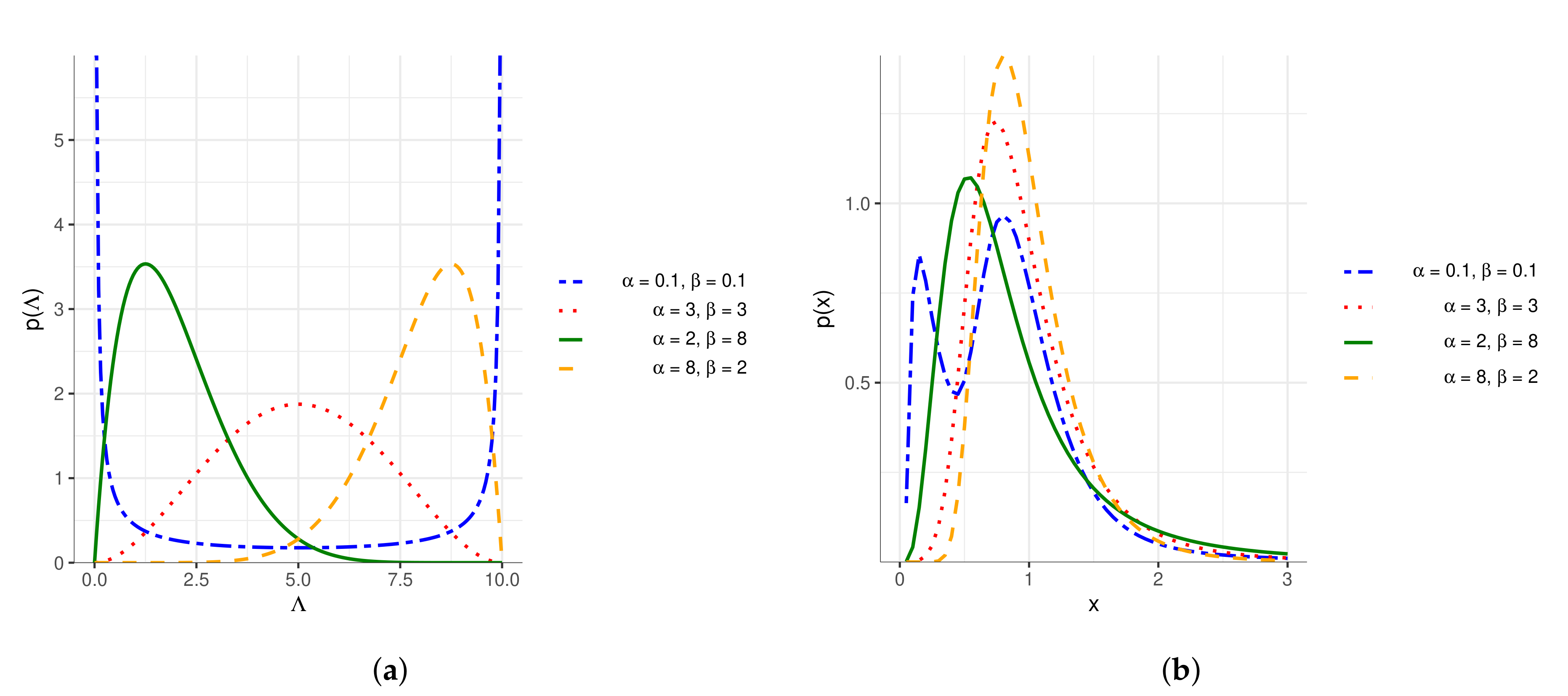
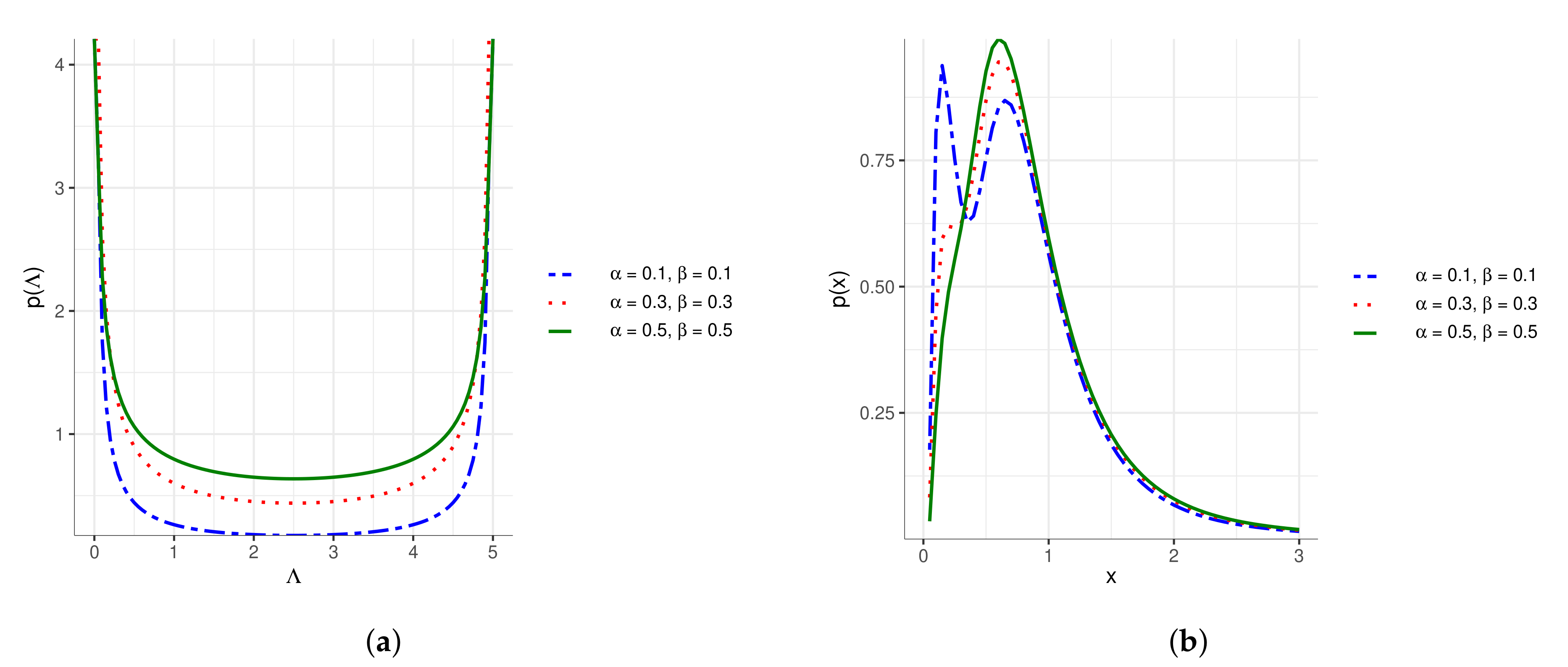
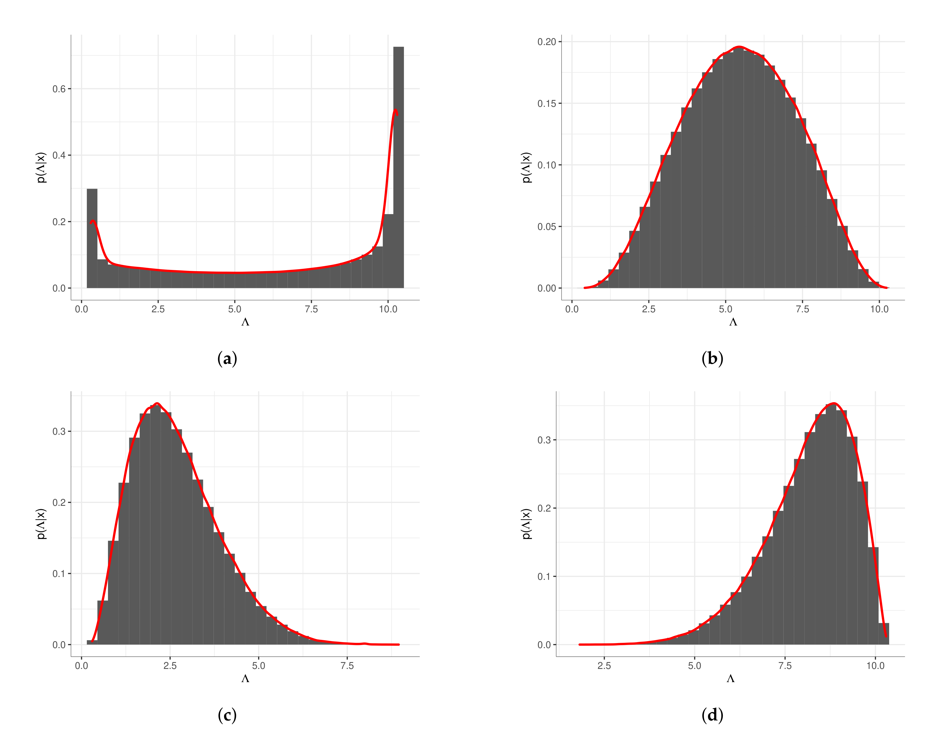
5.1. Estimation of the Marginal Function

The main goal of the numerical simulations is to understand how the shape of the inverse Gamma distribution (27) is affected by the choice of different Beta density functions used to sample the parameter $\mathrm{\Lambda }$.

Without loss of generality, we set in the inverse Gamma distribution (27) $\sigma$ equal to one, and we sample the parameter $\mathrm{\Lambda }$ from different Beta distributions. Figure 1a shows different Beta distributions based on different values of its parameters $\alpha$ and $\beta$. Notice that a Beta distribution with parameters $\alpha <1$ and $\beta <1$ represents a situation in which opinions are polarized, while in the other three cases considered in Figure 1a, the opinions are distributed around a modal value.

In order to estimate the marginal function of Equation (31), $N=1000$ different values of parameter $\mathrm{\Lambda }$ are sampled from each of the three Beta distribution, and the inverse Gamma distribution for each of the $\mathrm{\Lambda }$ values is computed. Finally, the average of these $N=1000$ inverse Gamma distributions is plotted in Figure 1b. This picture represents the estimated marginal function, i.e., the resulting wealth distribution.

We remark that all the results were obtained by changing the support of the Beta distribution in the following way:

• The support was shifted by 0.3 (which in the case of the function (27) is the value of the parameter $\delta$).
• The support was multiplied by a factor equal to 10 to highlight the shape of the wealth distribution.

A well-visible segregation case is obtained by fixing $\alpha =0.1$ and $\beta =0.1$, which describes a polarized situation. The corresponding Beta distribution has two defined peaks, which represent the two polarized opinions of the traders: one more conservative and the other one more inclined to invest. As a result, the marginal wealth distribution obtained by numerical simulation shows a bimodal shape, clearly visible in Figure 1b. On the other side, if we consider a Beta distribution characterized by only one peak, the corresponding marginal wealth distribution presents the classical unimodal shape.

On the basis of these results, it is possible to connect the shape of the wealth distribution with the distribution of the saving propensity, as given by resorting to the opinion formation model of Section 2.

To best clarify the relationship between the shape of the wealth distribution and the shape of the opinion distribution, one can resort to a sensitivity analysis in terms of the parameters of the Beta distribution and of the length of the support of the saving parameter $\mathrm{\Lambda }$. In Figure 2b, different shapes of the wealth distribution are shown. The bimodal shape is more evident only in the case of small values of the Beta distribution parameters. This is due to the fact that small values of $\alpha$ and $\beta$ correspond to an opinion distribution more polarized into two extreme values, as depicted in Figure 2a.

Figure 3 describes the shapes of the wealth distribution based on different values of the length support. A larger support of the saving parameter $\mathrm{\Lambda }$ implies a strong distinction between the extreme opinions described by the Beta distribution and, as a consequence, produces two defined peaks in the wealth distribution. On the opposite side, a small support represents a weaker distinction between two different opinions and implies a unimodal behavior.

Lastly, in Figure 4, we present the Lorenz curves corresponding to different choices of prior Beta distributions; see also [38,64]. The Lorenz curve is defined as:

$$L\left(F\left(w\right)\right)={\int }_0^2{f}_{\infty }\left(w_{*}\right)w_{*}d{w}_{*},$$

where $F\left(w\right)={\int }_0^w{f}_{\infty }\left(w_{*}\right)d{w}_{*}$ is the cumulative density function. Once having defined the Lorenz curve, we can compute the so-called Gini index as follows:

$$G_1=1-2{\int }_0^{1}L\left(x\right)dx.$$

This coefficient can be understood as an indicator of the inequality of a country, and it can be easily seen that it varies in $[0,1]$. In Western economies, a Gini index between $0.2$ and $0.5$ has been often measured.

In the present setup, one can observe in

Table 1. Gini index for each inverse Gamma distribution derived from the corresponding Beta distribution with parameters shown in the legend.

Prior Parameters	Gini Index
$\alpha =0.1$, $\beta =0.1$	0.55
$\alpha =3$, $\beta =3$	0.61
$\alpha =2$, $\beta =8$	0.56
$\alpha =8$, $\beta =2$	0.67

that in the presence of a radicalized situation, the measure of the area included between the diagonal and the curve is smaller for small values of the parameters $\alpha$ and $\beta$, which corresponds to a Gini index that is smaller in radicalized situations than in normal ones.

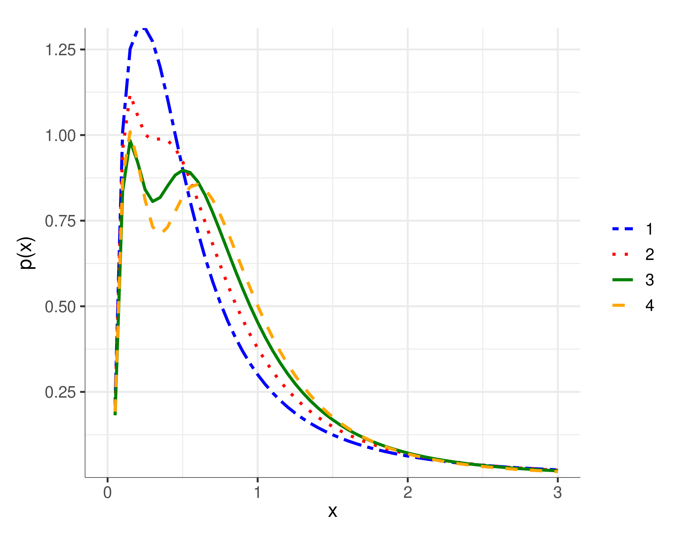
5.2. Estimation of the Posterior Function

As described in Section 4, this problem can be solved in the Bayesian framework. This allows us to compute the posterior distribution function using data and prior opinion.

In order to compute the posterior density function, the Metropolis–Hastings algorithm has been implemented [81]. The number of iterations was set equal to 1000. Figure 5 depicts the posterior estimation obtained according to four different prior distributions elicited with different values.

Note that in the case of a Beta distribution with $\alpha =0.1$ and $\beta =0.1$, namely in the case of our prior choice, we obtain a posterior estimation very unbalanced with respect to the initial prior choice. The shape of Figure 5a is indeed very close to a Beta distribution, but one of the two extreme opinions is more pronounced than the other. On the contrary, in the other three examples, the posterior distributions present a behavior analogous to the prior distributions.

The Anderson–Darling test performed on a random under-sampling of the observation generated confirms that in all four cases, the resulting posterior distribution is again a Beta distribution (p > 0.05).

Table 2. Estimation of the posterior parameters of the Beta distribution fixing the prior distribution.

Prior Parameters	Posterior Parameters
$\alpha =0.1$, $\beta =0.1$	$\widehat{\alpha }=0.41$, $\widehat{\beta }=0.22$
$\alpha =3$, $\beta =3$	$\widehat{\alpha }=3.41$, $\widehat{\beta }=3.17$
$\alpha =2$, $\beta =8$	$\widehat{\alpha }=2.62$, $\widehat{\beta }=8.33$
$\alpha =8$, $\beta =2$	$\widehat{\alpha }=8.28$, $\widehat{\beta }=2.23$

shows how the parameters of the posterior Beta distribution change with respect to the parameters of the prior Beta distribution.

6. Conclusions

We studied in this paper the consequences of stressful situations in the wealth distribution profile by considering a random saving propensity in the form of a Beta distribution. This choice is consistent with the opinion formation model developed in [65] and takes into account a general class of saving propensities, which range from the normal situation in which all agents in the society apply the same strategy to trade, to the extremal situation in which agents in the society split into two distinct classes, each using a constant saving propensity, but with marked differences between the two. It is subsequently shown that in highly stressful situations, one can observe the formation of a bimodal profile, which determines a marked emptying of the middle class. The statistical analysis of the random profile of the wealth distribution then shows that the choice of a Beta distribution allows obtaining most of the characteristic wealth distribution profiles observed in real economies. The analysis of the present paper seems very well adapted to study the consequences on the economy of a lockdown strategy, which naturally determines a splitting of the population on the basis of the immediate consequences on wealth of the part of the population that relies on an economy based on social contacts. Furthermore, the present analysis indicates that the model could be used as an early warning system for stressful economic situations, by regularly studying the effects of a trading activity in which the uncertain saving propensity parameter is built starting from well-targeted statistics on the population’s opinion.

References

1. Bassetti, F.; Toscani, G. Explicit equilibria in a kinetic model of gambling. Phys. Rev. E 2010, 81, 066115. [Google Scholar] [CrossRef] [PubMed] [Green Version]
2. Bassetti, F.; Toscani, G. Explicit equilibria in bilinear kinetic models for socio-economic interactions. ESAIM Proc. Surv. 2014, 47, 1–16. [Google Scholar] [CrossRef] [Green Version]
3. Bisi, M.; Spiga, G.; Toscani, G. Kinetic models of conservative economies with wealth redistribution. Commun. Math. Sci. 2009, 7, 901–916. [Google Scholar] [CrossRef] [Green Version]
4. Cáceres, M.J.; Toscani, G. Kinetic approach to long time behavior of linearized fast diffusion equations. J. Stat. Phys. 2007, 128, 883–925. [Google Scholar] [CrossRef]
5. Chatterjee, A.; Chakrabarti, B.K.; Manna, S.S. Pareto law in a kinetic model of market with random saving propensity. Physica A 2004, 335, 155–163. [Google Scholar] [CrossRef] [Green Version]
6. Chatterjee, A.; Chakrabarti, B.K.; Stinchcombe, R.B. Master equation for a kinetic model of trading market and its analytic solution. Phys. Rev. E 2005, 72, 026126. [Google Scholar] [CrossRef] [Green Version]
7. Chakraborti, A. Distributions of money in models of market economy. Int. J. Mod. Phys. C 2002, 13, 1315–1321. [Google Scholar] [CrossRef] [Green Version]
8. Chakraborti, A.; Chakrabarti, B.K. Statistical mechanics of money: How saving propensity affects its distribution. Eur. Phys. J. B 2000, 17, 167–170. [Google Scholar] [CrossRef] [Green Version]
9. Cordier, S.; Pareschi, L.; Piatecki, C. Mesoscopic modelling of financial markets. J. Stat. Phys. 2009, 134, 161–184. [Google Scholar] [CrossRef] [Green Version]
10. Dragulescu, A.; Yakovenko, V.M. Statistical mechanics of money. Eur. Phys. J. B 2000, 17, 723–729. [Google Scholar] [CrossRef] [Green Version]
11. Düring, B.; Matthes, D.; Toscani, G. Kinetic equations modelling wealth redistribution: A comparison of approaches. Phys. Rev. E 2008, 78, 056103. [Google Scholar] [CrossRef] [PubMed] [Green Version]
12. Düring, B.; Matthes, D.; Toscani, G. A Boltzmann-type approach to the formation of wealth distribution curves. Riv. Mat. Univ. Parma 2009, 8, 199–261. [Google Scholar] [CrossRef] [Green Version]
13. Gupta, A.K. Models of wealth distributions: A perspective. In Econophysics and Sociophysics: Trends and Perspectives; Chakrabarti, A., Chakraborti, B.K., Chatterjee, A., Eds.; Wiley VHC: Weinheim, Germany, 2006; pp. 161–190. [Google Scholar]
14. Ispolatov, S.; Krapivsky, P.L.; Redner, S. Wealth distributions in asset exchange models. Eur. Phys. J. B 1998, 2, 267–276. [Google Scholar] [CrossRef] [Green Version]
15. Maldarella, D.; Pareschi, L. Kinetic models for socio–economic dynamics of speculative markets. Physica A 2012, 391, 715–730. [Google Scholar] [CrossRef] [Green Version]
16. Matthes, D.; Toscani, G. On steady distributions of kinetic models of conservative economies. J. Stat. Phys. 2008, 130, 1087–1117. [Google Scholar] [CrossRef]
17. Slanina, F. Inelastically scattering particles and wealth distribution in an open economy. Phys. Rev. E 2004, 69, 046102. [Google Scholar] [CrossRef] [PubMed] [Green Version]
18. Toscani, G.; Brugna, C.; Demichelis, S. Kinetic models for the trading of goods. J. Stat. Phys. 2013, 151, 549–566. [Google Scholar] [CrossRef] [Green Version]
19. Pareto, V. Cours d’Économie Politique; Librairie Droz: Geneva, Switzerland, 1964. [Google Scholar]
20. Bassetti, F.; Toscani, G. Mean field dynamics of collisional processes with duplication, loss and copy. Math. Mod. Meth. Appl. Sci. 2015, 25, 1887–1925. [Google Scholar] [CrossRef]
21. Carrillo, J.A.; Fornasier, M.; Rosado, J.; Toscani, G. Asymptotic flocking dynamics for the kinetic Cucker-Smale model. SIAM J. Math. Anal. 2010, 42, 218–236. [Google Scholar] [CrossRef] [Green Version]
22. Ha, S.-Y.; Jeong, E.; Kang, J.-H.; Kang, K. Emergence of multi-cluster configurations from attractive and repulsive interactions. Math. Models Methods Appl. Sci. 2012, 22, 1250013. [Google Scholar] [CrossRef]
23. Kashdan, E.; Pareschi, L. Mean field mutation dynamics and the continuous Luria-Delbrück distribution. Math. Biosci. 2012, 240, 223–230. [Google Scholar] [CrossRef] [PubMed] [Green Version]
24. Toscani, G. A kinetic description of mutation processes in bacteria. Kinet. Relat. Models 2013, 6, 1043–1055. [Google Scholar] [CrossRef]
25. Castellano, C.; Fortunato, S.; Loreto, V. Statistical physics of social dynamics. Rev. Mod. Phys. 2009, 81, 591–646. [Google Scholar] [CrossRef] [Green Version]
26. Chakrabarti, B.K.; Chakraborti, A.; Chakravarty, S.R.; Chatterjee, A. Econophysics of Income and Wealth Distributions; Cambridge University Press: Cambridge, UK, 2013. [Google Scholar]
27. Naldi, G.; Pareschi, L.; Toscani, G. Mathematical Modeling of Collective Behavior in Socio-Economic and Life Sciences; Springer: Berlin/Heidelberg, Germany, 2010. [Google Scholar]
28. Pareschi, L.; Toscani, G. Interacting Multiagent Systems. Kinetic Equations & Monte Carlo Methods; Oxford University Press: Oxford, UK, 2013. [Google Scholar]
29. Sen, P.; Chakrabarti, B.K. Sociophysics: An Introduction; Oxford University Press: Oxford, UK, 2014. [Google Scholar]
30. Herty, M.; Tosin, A.; Visconti, G.; Zanella, M. Reconstruction of traffic speed distributions from kinetic models with uncertainties. In Mathematical Descriptions of Traffic Flow: Micro, Macro and Kinetic Models; Tosin, A., Puppo, G., Eds.; Springer: Berlin/Heidelberg, Germany, 2019. [Google Scholar]
31. Piccoli, B.; Tosin, A.; Zanella, M. Model-based assessment of the impact of driver-assist vehicles using kinetic theory. arXiv 2019, arXiv:1911.04911. [Google Scholar]
32. Tosin, A.; Zanella, M. Uncertainty damping in kinetic traffic models by driver-assist controls. arXiv 2019, arXiv:1904.00257. [Google Scholar]
33. Tosin, A.; Zanella, M. Kinetic-controlled hydrodynamics for traffic models with driver-assist vehicles. Multiscale Model Simul. 2019, 17, 716–749. [Google Scholar]
34. Furioli, G.; Pulvirenti, A.; Terraneo, E.; Toscani, G. Non-Maxwellian kinetic equations modeling the evolution of wealth distribution. Math. Models Methods Appl. Sci. 2020, 30, 685–725. [Google Scholar] [CrossRef]
35. Bouchaud, J.F.; Mézard, M. Wealth condensation in a simple model of economy. Physica A 2000, 282, 536–545. [Google Scholar] [CrossRef] [Green Version]
36. Cordier, S.; Pareschi, L.; Toscani, G. On a kinetic model for a simple market economy. J. Stat. Phys. 2005, 120, 253–277. [Google Scholar] [CrossRef] [Green Version]
37. Bisi, M. Some kinetic models for a market economy. Boll. Unione Mat. Ital. 2017, 10, 143–158. [Google Scholar] [CrossRef]
38. Düring, B.; Pareschi, L.; Toscani, G. Kinetic models for optimal control of wealth inequalities. Eur. Phys. J. B 2018, 91, 265. [Google Scholar] [CrossRef] [Green Version]
39. Düring, B.; Toscani, G. Hydrodynamics from kinetic models of conservative economies. Physica A 2007, 384, 493–506. [Google Scholar] [CrossRef] [Green Version]
40. Düring, B.; Toscani, G. International and domestic trading and wealth distribution. Commun. Math. Sci. 2008, 6, 1043–1058. [Google Scholar] [CrossRef] [Green Version]
41. Torregrossa, M.; Toscani, G. Wealth distribution in presence of debts. A Fokker–Planck description. Commun. Math. Sci. 2018, 16, 537–560. [Google Scholar] [CrossRef] [Green Version]
42. Bobylëv, A.V. The method of the Fourier transform in the theory of the Boltzmann equation for Maxwell molecules. Dokl. Akad. Nauk SSSR 1975, 225, 1041–1044. [Google Scholar]
43. Cercignani, C. The Boltzmann Equation and Its Applications; Springer Series in Applied Mathematical Sciences; Springer: New York, NY, USA, 1988; Volume 67. [Google Scholar]
44. Dolfin, M.; Leonida, L.; Outada, N. Modeling human behavior in economics and social science. Phys. Life Rev. 2017, 22–23, 1–21. [Google Scholar] [CrossRef] [PubMed] [Green Version]
45. Furioli, G.; Pulvirenti, A.; Terraneo, E.; Toscani, G. Fokker–Planck equations in the modelling of socio-economic phenomena. Math. Models Methods Appl. Sci. 2017, 27, 115–158. [Google Scholar] [CrossRef] [Green Version]
46. Torregrossa, M.; Toscani, G. On a Fokker–Planck equation for wealth distribution. Kinet. Relat. Models 2018, 11, 337–355. [Google Scholar] [CrossRef] [Green Version]
47. Toscani, G. Entropy dissipation and the rate of convergence to equilibrium for the Fokker–Planck equation. Quart. Appl. Math. 1999, LVII, 521–541. [Google Scholar] [CrossRef] [Green Version]
48. Toscani, G.; Villani, C. Sharp entropy dissipation bounds and explicit rate of trend to equilibrium for the spatially homogeneous Boltzmann equation. Commun. Math. Phys. 1999, 203, 667–706. [Google Scholar] [CrossRef]
49. Villani, C. A Review of Mathematical Topics in Collisional Kinetic Theory. In Handbook of Mathematical Fluid Dynamics; Friedlander, S., Serre, D., Eds.; Elsevier: New York, NY, USA, 2002; Volume 1. [Google Scholar]
50. Albi, G.; Pareschi, L.; Zanella, M. Uncertainty quantification in control problems for flocking models. Math. Probl. Eng. 2015, 15, 850124. [Google Scholar] [CrossRef] [Green Version]
51. Bellomo, N.; Colasuonno, F.; Knopoff, D.; Soler, J. From a systems theory of sociology to modeling the onset and evolution of criminality. Netw. Heterog. Media 2015, 10, 421–441. [Google Scholar] [CrossRef]
52. Bellomo, N.; Herrero, M.A.; Tosin, A. On the dynamics of social conflicts looking for the Black Swan. Kinet. Relat. Models 2013, 6, 459–479. [Google Scholar] [CrossRef] [Green Version]
53. Bellomo, N.; Soler, J. On the mathematical theory of the dynamics of swarms viewed as complex systems. Math. Models Methods Appl. Sci. 2012, 22, 1140006. [Google Scholar] [CrossRef]
54. Gualandi, S.; Toscani, G. Pareto tails in socio-economic phenomena: A kinetic description. Economics 2018, 12, 1–17. [Google Scholar] [CrossRef] [Green Version]
55. Gualandi, S.; Toscani, G. Human behavior and lognormal distribution. A kinetic description. Math. Models Methods Appl. Sci. 2019, 29, 717–753. [Google Scholar] [CrossRef] [Green Version]
56. Chatterjee, A.; Chakrabarti, B.K.; Manna, S.S. Money in gas-like markets: Gibbs and Pareto laws. Phys. Scr. 2003, 106, 36. [Google Scholar] [CrossRef] [Green Version]
57. Lim, G.; Min, S. Analysis of solidarity effect for entropy, Pareto, and Gini indices on two-class society using kinetic wealth exchange model. Entropy 2020, 22, 386. [Google Scholar] [CrossRef] [Green Version]
58. Patriarca, M.; Chakraborti, A.; Kaski, K.; Germano, G. Kinetic theory models for the distribution of wealth: Power law from overlap of exponentials. In Econophysics of Wealth Distributions; Chatterjee, A., Yarlagadda, S., Chakrabarti, B.K., Eds.; Springer: Berlin/Heidelberg, Germany, 2005; pp. 93–110. [Google Scholar]
59. Patriarca, M.; Chakraborti, A.; Germano, G.O. Influence of saving propensity on the power-law tail of the wealth distribution. Physica A 2006, 369, 723–736. [Google Scholar] [CrossRef] [Green Version]
60. Ghosh, A.; Chatterjee, A.; Inoue, J.I.; Chakrabarti, B.K. Inequality measures in kinetic exchange models of wealth distributions. Physica A 2016, 451, 465–474. [Google Scholar] [CrossRef] [Green Version]
61. Ferrero, J.C. The monomodal, polymodal, equilibrium and nonequilibrium distribution of money. In Econophysics of Wealth Distributions; Chatterjee, A., Yarlagadda, S., Chakrabarti, B.K., Eds.; Springer: Cernusco, Italy, 2005; pp. 159–167. [Google Scholar]
62. Ferrero, J.C. The individual income distribution in Argentina in the period 2000–2009. A unique source of non stationary data. arXiv 2010, arXiv:1006.2057. [Google Scholar]
63. Bellomo, N.; Bingham, R.; Chaplain, M.A.; Dosi, G.; Forni, G.; Knopoff, D.A.; Lowengrub, J.; Twarock, R.; Virgillito, M.E. A Multi-Scale Model of Virus Pandemic: Heterogeneous Interactive Entities in a Globally Connected World. Math. Mod. Meth. Appl. Sci. 2020. [Google Scholar] [CrossRef]
64. Dimarco, G.; Pareschi, L.; Toscani, G.; Zanella, M. Wealth distribution under the spread of infectious diseases. Phys. Rev. E 2020, 102, 022303. [Google Scholar] [CrossRef]
65. Toscani, G. Kinetic models of opinion formation. Commun. Math. Sci. 2006, 4, 481–496. [Google Scholar] [CrossRef] [Green Version]
66. Pareschi, L.; Toscani, G.; Tosin, A.; Zanella, M. Hydrodynamics models of preference formation in multi-agent societies. J. Nonlin. Sci. 2019, 29, 2761–2796. [Google Scholar] [CrossRef] [Green Version]
67. Toscani, G.; Tosin, A.; Zanella, M. Opinion modeling on social media and marketing aspects. Phys. Rev. E 2018, 98, 022315. [Google Scholar] [CrossRef] [PubMed] [Green Version]
68. Albi, G.; Pareschi, L.; Zanella, M. Opinion dynamics over complex networks: Kinetic modelling and numerical methods. Kinet. Relat. Models 2017, 10, 1–32. [Google Scholar] [CrossRef] [Green Version]
69. Ben-Naim, E. Opinion dynamics: Rise and fall of political parties. Europhys. Lett. 2005, 69, 671–677. [Google Scholar] [CrossRef] [Green Version]
70. Ben-Naim, E.; Krapivsky, P.L.; Redner, S. Bifurcation and patterns in compromise processes. Physica D 2003, 183, 190–204. [Google Scholar] [CrossRef] [Green Version]
71. Ben-Naim, E.; Krapivsky, P.L.; Vazquez, F.; Redner, S. Unity and discord in opinion dynamics. Physica A 2003, 330, 99–106. [Google Scholar] [CrossRef]
72. Weisbuch, G.; Deffuant, G.; Amblard, F. Persuasion dynamics. Physica A 2005, 353, 555–575. [Google Scholar] [CrossRef] [Green Version]
73. Furioli, G.; Pulvirenti, A.; Terraneo, E.; Toscani, G. Wright–Fisher–type equations for opinion formation, large time behavior and weighted Logarithmic–Sobolev inequalities. Ann. IHP Anal. Non Linéaire 2019, 36, 2065–2082. [Google Scholar] [CrossRef] [Green Version]
74. Villani, C. Contribution à L’étude Mathématique des Équations de Boltzmann et de Landau en théorie Cinétique des gaz et des Plasmas. Ph.D. Thesis, Univ. Paris-Dauphine, Paris, France, 1998. [Google Scholar]
75. Villani, C. On a new class of weak solutions to the spatially homogeneous Boltzmann and Landau equations. Arch. Ration. Mech. Anal. 1998, 143, 273–307. [Google Scholar] [CrossRef]
76. Tosin, A.; Zanella, M. Boltzmann-type models with uncertain binary interactions. Commun. Math. Sci. 2018, 16, 962–984. [Google Scholar] [CrossRef] [Green Version]
77. Kac, M. Probability and Related Topics in the Physical Sciences; New York Interscience: London, UK, 1959. [Google Scholar]
78. Carrillo, J.A.; Pareschi, L.; Zanella, M. Particle based gPC methods for mean-field models of swarming with uncertainty. Commun. Comput. Phys. 2019, 25, 508–531. [Google Scholar] [CrossRef]
79. Carrillo, J.A.; Pareschi, L.; Zanella, M. Monte Carlo gPC methods for diffusive kinetic flocking models with uncertainties. Viet. J. Math. 2019, 47, 931–954. [Google Scholar] [CrossRef] [Green Version]
80. Bernardo, J.M.; Smith, A.F.M. Bayesian Theory; John Wiley and Sons: Chichester, UK, 2009. [Google Scholar]
81. Hastings, W.K. Monte Carlo sampling methods using Markov chains and their applications. Biometrik 1970, 57, 97–109. [Google Scholar] [CrossRef]
Figure 1. (a) Beta probability distribution functions plotted for different values of parameters α and β .(b) marginal distribution functions computed for each of the Beta distributions.
Symmetry 12 01390 g001
Figure 2. We report the sensitivity analysis on the marginal distribution in (b) performed for different parameters of the Beta distribution in (a) obtained for the length of the support fixed to five.
Symmetry 12 01390 g002
Figure 3. Sensitivity analysis performed on different values of the length of the support using a Beta density function with α = 0.1 , β = 0.1 as the opinion distribution.
Symmetry 12 01390 g003
Figure 4. Lorenz curve computed for each prior Beta distribution.
Symmetry 12 01390 g004
Figure 5. Posterior estimation through Metropolis–Hastings for different prior distributions: (a) Beta distribution with parameters α = 0.1 and β = 0.1 , (b) Beta distribution with parameters α = 3 and β = 3 , (c) Beta distribution with parameters α = 2 and β = 8 , (d) Beta distribution with parameters α = 8 and β = 2 .
Symmetry 12 01390 g005