Article

On Taylor Series Expansion for Statistical Moments of Functions of Correlated Random Variables †

Faculty of Civil Engineering, Brno University of Technology, 60200 Brno, Czech Republic
*
Author to whom correspondence should be addressed.
This paper is an extended version of our paper published in The 17th international Conference of Numerical Analysis and Applied Mathematics (ICNAAM 2019).
Symmetry 2020, 12(8), 1379; https://doi.org/10.3390/sym12081379
Submission received: 29 July 2020 / Revised: 15 August 2020 / Accepted: 17 August 2020 / Published: 18 August 2020

Abstract

:
The paper is focused on Taylor series expansion for statistical analysis of functions of random variables with special attention to correlated input random variables. It is shown that the standard approach leads to significant deviations in estimated variance of non-linear functions. Moreover, input random variables are often correlated in industrial applications; thus, it is crucial to obtain accurate estimations of partial derivatives by a numerical differencing scheme. Therefore, a novel methodology for construction of Taylor series expansion of increasing complexity of differencing schemes is proposed and applied on several analytical examples. The methodology is adapted for engineering applications by proposed asymmetric difference quotients in combination with a specific step-size parameter. It is shown that proposed differencing schemes are suitable for functions of correlated random variables. Finally, the accuracy, efficiency, and limitations of the proposed methodology are discussed.

1. Introduction

Mathematical modeling in civil engineering is often represented by the finite element method (FEM). Although FEM is an accurate and efficient technique, it is still highly time-consuming, particularly in the case of non-linear FEM including geometrical and material non-linearity. Therefore, from a practical point of view, it is necessary to decrease the number of FEM calculations as much as possible while satisfying the given safety requirements of the analyzed structure. A solution can be represented by a semi-probabilistic approach widely accepted in the engineering field [1] and implemented into the national codes such as Eurocode [2]. Such approach is able to greatly reduce the number of necessary calculations for the design and an assessment of structures. The basic reliability concept is given as Z = R E , where Z is a safety margin, which is defined as the difference between the structural resistance R and the load effect E. The task of reliability analysis is the estimation of failure probability p f = P Z < 0 , which might be highly computationally demanding. According to the semi-probabilistic approach, the resistance of a structure R is separated, and the design value R d satisfying given safety requirements is evaluated instead of calculating the failure probability. Such approach directly leads to the design value of resistance, which is obtained by the traditional Partial Safety Factor (PSF) approach, and thus can be easily used for a design and an assessment of structures. The PSF method is based on a simple assumption, that a calculation with design values of input random variables leads to the design value of resistance R d = r x d , where design values of input random variables x d are derived under several simplifications, such as a linearization of a limit state function. In consequence, PSF works well for standard linear calculations, but there may be a significant error for a non-linear analysis, which is far more popular nowadays. Therefore, it is necessary to develop new methods in compliance with the semi-probabilistic approach applicable for non-linear analysis. The semi-probabilistic approach is briefly presented in the following paragraph.
It is assumed that R and E are independent, and separated R is lognormally distributed; thus, the design value of resistance R d is defined as
R d = μ R · e x p ( α R β v R ) ,
where v R is the coefficient of variation (CoV) of resistance, and α R represents the sensitivity factor associated with R derived from the First Order Reliability Method (FORM) [1,3]. FORM is commonly applied to linearization of limit state function at the most probable failure point by Taylor series expansion. FORM assumes the uncorrelated standardized Gaussian space ξ ; thus, all variables must be transformed by Rosenblatt transformation [4] from the original space. The coordinates of the most probable failure point, also called the design point, are thereafter described by the shortest distance β to the origin of the ξ space, direction cosines α R associated with resistance and α E associated with load. The shortest distance β is defined as the Hasofer–Lind reliability index, and its minimal value is given for various conditions in normative documents, in order to achieve the target safety of structures.
For industrial applications, FORM is simplified by the statistical estimation of fixed value α R = 0.8 . Therefore, to determine the design value by a semi-probabilistic approach, it is crucial to correctly estimate the mean value and variance of structural resistance R, which can be seen as a function of multiple random variables. This task may be challenging due to the fact that input random variables can generally be non-Gaussian and correlated. There have been several methods proposed in last two decades to estimate the variation coefficient of R (ECoV methods) [5,6,7,8,9,10]; however, mathematical background and limitations of these methods are often missing, and there is no solution for correlated random variables, which is common for material characteristics.
The only general approach to estimate statistical moments is pseudo-random sampling by a Monte Carlo type algorithm such as Crude Monte Carlo or Latin Hypercube Sampling [11,12] employed in numerical examples as a reference solution. However, it is necessary to perform a high number of simulations of the original mathematical model, which is not feasible in industrial applications due to the enormous computational burden. On the other hand, it is possible to assume several simplifications and create an approximation of the original mathematical model of R.
The approximating function is called a surrogate model, or a metamodel, and it is a topic of great interest among researchers from various research fields. The Polynomial Chaos Expansion (PCE) is often used for uncertainty quantification [13,14]. The Gaussian process or Krigging has recently received significant attention in reliability analysis of systems with very low failure probabilities [15], and artificial neural networks are often utilized for reliability-based optimization [16]. Although PCE, Krigging, and ANN represent very powerful and efficient approaches with many advantages, these advanced techniques require deep knowledge of theoretical background, and it is necessary to use developed algorithms with great caution.
Another well-known approximation of functions is Taylor series expansion (TSE), which was also used for derivation of PSF and FORM as described, for example, in [17]. Although TSE is often used to estimate statistical moments of functions of random variables by mathematicians, it has not yet been well investigated in the context of non-linear FEM in civil engineering in order to adapt and directly use TSE for structural reliability and semi-probabilistic approaches. For industrial applications, it is crucial that the proposed methods are easy to implement and easy to use with the same level of knowledge about the mathematical model as in the case of PSF. Therefore, it makes perfect sense to generalize TSE, which is already utilized for the derivation of PSF implemented in codes, to directly use in combination with FEM and semi-probabilistic ECoV approach. Therefore, the ECoV method based on TSE adapted for civil engineers is discussed, and several modifications of this approach are proposed in the next section. Moreover, the whole methodology of increasing complexity and accuracy of TSE suitable for industrial applications is proposed in this paper.

2. Taylor Series Expansion

An original mathematical model is often highly time-consuming, and it is necessary to create an approximation—a simplified function in explicit form. Although there are several advanced types of surrogate models, it is still common to use the traditional approach, called Taylor series expansion, which can be truncated to arbitrary order and used with various differencing schemes. Although such adaptivity makes TSE a powerful technique, there are severe problems for practical computations in the case of non-linear functions with complex stochastic models containing a dependence structure. In the following paragraphs, let us assume an original mathematical model in form of software algorithm (e.g., FEM); thus, the derivatives must be calculated numerically.
Let ( Ω , F , P ) be a probability space, where Ω is an event space, F is Borel σ -algebra on Ω , and P is a probability measure P : F 0 , 1 . Let us assume a random vector X = X 1 , X 2 , X n T consisting of random variables X ( ω ) , ω Ω with existing mean values μ X 1 , μ X 2 , , μ X n and a mathematical model of this input random vector r X . The response of the mathematical model is thereafter a random variable R described by a specific probability distribution and statistical moments. Further, let us assume the mathematical model r X to be infinitely differentiable in some open interval around the vector of mean values μ X = μ X 1 , μ X 2 , , μ X n . Under this assumption, it is possible to expand the original model to the infinite Taylor series according to Taylor’s theorem:
r ( X ) = r ( μ X ) + r ( μ X ) · ( X μ X ) + 1 2 ( X μ X ) · r ( μ X ) · ( X μ X ) + · · · = = r μ X 1 , μ X 2 , , μ X n + i = 1 n r ( X ) X i X i μ X i + 1 2 i = 1 n j = 1 n 2 r ( X ) X i X j X i μ X i X j μ X j +
where the derivatives are evaluated at μ X 1 , μ X 2 , , μ X n . Note that TSE consists of a constant term, linear term, quadratic term, etc. For a practical computation, it is crucial to reduce Taylor series to a finite number of terms and to obtain derivatives by numerical differentiation. There are many possible differencing schemes, which are more or less suitable for specific applications. One of the possible formulas for numerical derivation was proposed by Schlune et al. [9], especially for civil engineers, where derivatives are approximated by the asymmetric difference quotient as follows:
r ( X ) X i = R X m R X i Δ Δ X i .
where the response of mathematical model R X m is a calculation with mean values of X, and R X i Δ is the result of the model using reduced mean values of the i-th input random variables by Δ X i . This differencing scheme is adapted for a structural design and an assessment by the step-size parameter c = ( α R β ) / 2 , and X i Δ corresponds to quantile F i 1 ( Φ ( c ) ) , where F i 1 is an inverse cumulative distribution function of the i-th variable, and Φ is the cumulative distribution function of standardized Gaussian distribution. For the sake of clarity, the difference is calculated as Δ X i = X i m X i Δ . Note that the step-size parameter is a function of the reliability index; thus, it is in compliance with the philosophy of a semi-probabilistic approach implemented in civil engineering codes [1]. Following this idea, additional asymmetric differencing schemes adapted for civil engineering used in combination with TSE of the first and the second order are proposed in the following subsections.

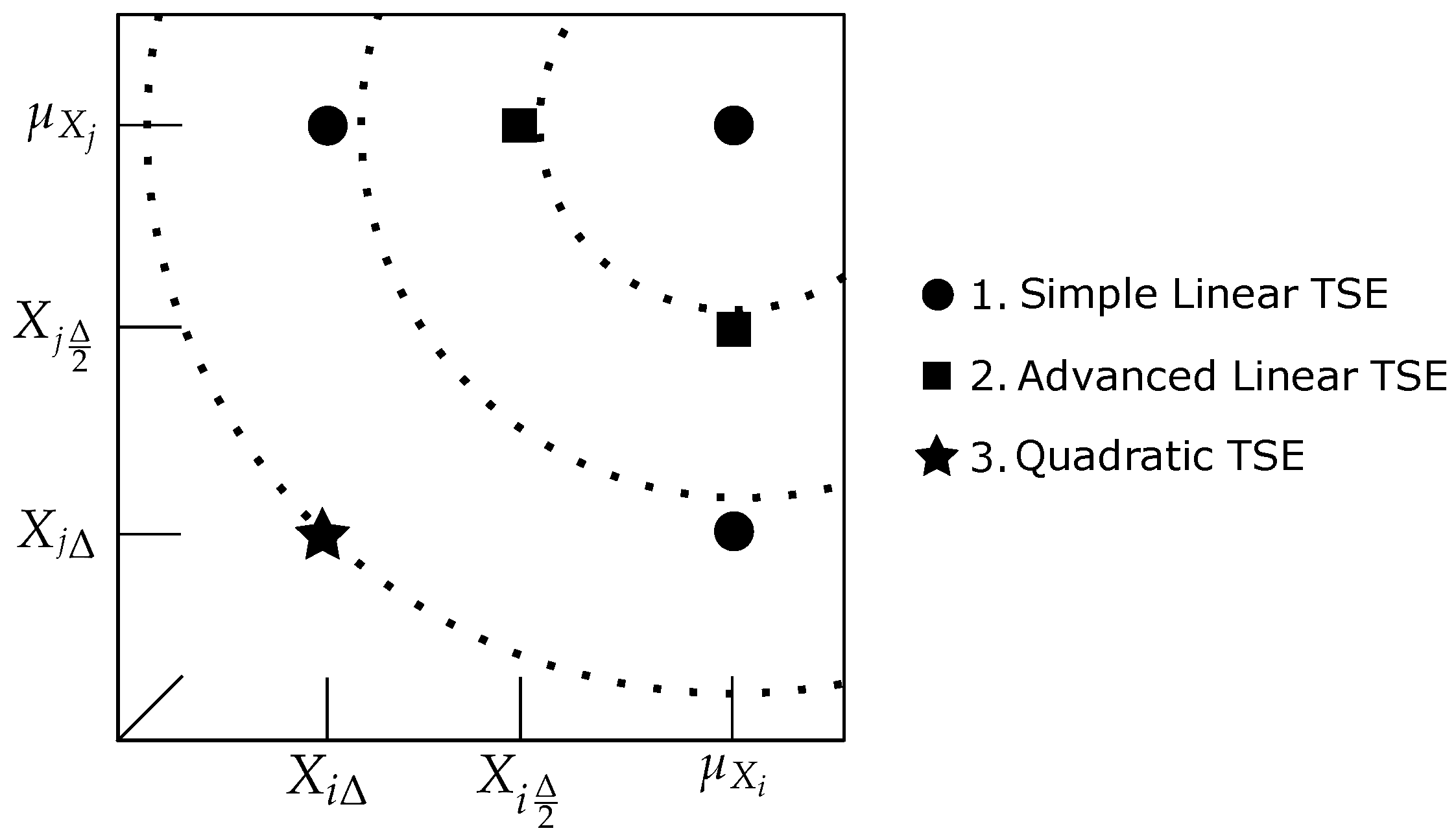
2.1. Linear Terms of Taylor Series Expansion

In engineering applications, it is common to assume only linear terms of TSE and independent input random variables. Since a semi-probabilistic approach is focused on practical applications, the significant advantage of TSE reduced to linear terms is the possibility of analyzing expressions for an expected value and a variance, see e.g., [17].
Theorem 1.
If an original mathematical function r : R n R of n independent random variables described by mean value μ X i and variance σ X i 2 is approximated by Taylor series expansion reduced to linear terms, the first two statistical moments of the response R T of linear Taylor approximation are analytically obtained as follows:
E R T r μ X
V a r R T i = 1 n r ( X ) X i 2 σ X i 2
Proof of Theorem 1.
For the sake of clarity, the estimations of expected value E R T and variance V a r R T for the function of n independent random variables are as follows:
E R T E r μ X 1 , μ X 2 , , μ X n + i = 1 n E r ( X ) X i X i μ X i r μ X 1 , μ X 2 , , μ X n
and
V a r R T V a r r μ X 1 , μ X 2 , , μ X n + i = 1 n r ( X ) X i X i μ X i = i = 1 n V a r r ( X ) X i X i μ X i + + i , j = 1 , , N i j C o v r ( X ) X i X i μ X i , r ( X ) X j X j μ X j = i = 1 n r ( X ) X i 2 σ X i 2
where the final equation arises from the definition of variance V a r ( X ) = σ X 2 = E X μ 2 and property of variance V a r ( c X i + d X j ) = c 2 V a r ( X i ) + d 2 V a r ( X j ) + 2 c d C o v ( X i , X j ) . Moreover, for independent variables, the covariance between variables is equal to zero, and thus the formula is reduced.  □
As can be seen from the proof above, there is a strict assumption of uncorrelated random variables for Equation (5). However, it is necessary to assume correlated random variables in some practical examples solved by FEM to represent realistic behaviors of structures. An extension of the method for dependent random variables can be obtained from the proof above using first-order Taylor series expansion assuming correlation among random variables represented by the correlation coefficient ρ in analytical form as
V a r R T i = 1 n r ( X ) X i 2 σ X i 2 + i , j = 1 , , n i j ρ i , j σ X i σ X j r ( X ) X i r ( X ) X j .
However, higher terms of TSE or more accurate approximation of derivatives should be considered for the correct estimation of variance in the case of dependent input random variables and non-linear functions. Otherwise, the correlation term may lead to significant inaccuracy of the resulting variance. We propose the second-order backward asymmetric differencing according to Equation (9), which is adapted for structural design utilizing the parameter c = ( α R β ) / 2 analogously to Equation (3) proposed by Schlune et al. The middle additional term R X i Δ 2 is obtained by an evaluation of the original mathematical model with reduced i-th variable X i Δ 2 = X i m Δ X i / 2 . Note that the proposed approach needs 2 n + 1 evaluations of the original model, while the scheme proposed by Schlune needs n + 1 simulations. In practice, an analyst could use the derivative scheme according to Schlune and further compute additional n simulations in order to obtain R X i Δ 2 and more accurate results.
r ( X ) X i = 3 R X m 4 R X i Δ 2 + R X i Δ Δ X i .

2.2. Higher-Order Taylor Series Expansion

If higher terms of TSE are considered, it is inefficient to derive analytical formulas for statistical moments [18], and thus mean and variance should be calculated numerically by simulation techniques directly from Equation (2) truncated to quadratic terms. Moreover, additional higher-order derivatives must be evaluated, which might not be feasible in computationally demanding practical examples. Therefore, linear TSE is preferred for practical computations. However, for specific cases with significant interaction of input variables, one may use second-order TSE for the estimation of coefficient of variation. In this case, it is necessary to compute all second-order partial derivatives. For numerical calculations of 2 r ( X ) X i 2 , it is possible to use the already defined simulations R X m , R X i Δ , R X i Δ 2 in a standard asymmetric backward differencing scheme:
2 r ( X ) X i X i = R X m 2 R X i Δ 2 + R X i Δ Δ X i 2
The only additional computations of the original mathematical model needed are for mixed partial derivatives 2 r ( X ) X i X j . Note that it is necessary to perform additional n 2 simulations in order to obtain all the mixed partial derivatives. In total, it is necessary to calculate 2 n + n 2 + 1 simulations for second-order TSE using the proposed asymmetric differencing schemes.
Theorem 2.
Mixed partial derivatives can be approximated by the simple backward finite differencing as
2 r ( X ) X i X j = R X m R X i Δ R X j Δ + R X i Δ X j Δ Δ X i Δ X j ,
where R X i Δ X j Δ represents the response of a mathematical model with reduced mean values of both i-th and j-th input random variables. All other variables were defined in the previous differencing schemes.
Proof of Theorem 2.
Using the simple one-sided backward differencing defined by Equation (3), one can derive mixed partial derivatives as follows:
2 r X i X j r ( X ) X j μ X i , μ X j r ( X ) X j X i Δ , μ X j Δ X i
where r ( X ) X j is computed for specific coordinates μ X i , μ X j and X i Δ , μ X j as
r ( X ) X j μ X i , μ X j R X m R X j Δ Δ X j
and
r ( X ) X j X i Δ , μ X j R X i Δ R X i Δ X j Δ Δ X j
Therefore, the final derivative scheme for mixed second partial derivatives based on the simple backward differencing adapted for a semi-probabilistic approach is
2 r ( X ) X i X j = R X m R X i Δ R X j Δ + R X i Δ X j Δ Δ X i Δ X j
 □

3. Numerical Computation

3.1. Methodology of ECoV by TSE

Since TSE can be constructed in various forms, it is beneficial to create ECoV methodology using TSE, composed of the three levels of an approximation using asymmetric differencing schemes already described in the previous section in combination with linear and quadratic TSE as follows:
(1)
linear TSE with a simple differencing scheme using Equation (3)— n s i m = n + 1 ,
(2)
linear TSE with an advanced differencing scheme using Equation (9)— n s i m = 2 n + 1 ,
(3)
TSE truncated to quadratic terms with a differencing scheme using Equation (9) for the first-order derivatives, Equation (10) for the second-order partial derivatives, and Equation (11) for the mixed derivatives—number of calculation is n s i m = 2 n + n 2 + 1 in total.
The first level was proposed by Schlune et al. [9] for uncorrelated random variables, and it was used in several practical studies [19,20,21]. However, its behavior for functions of correlated input random variables has not been investigated yet, though it is often necessary to assume correlated random material characteristics in industrial applications. It can be expected that the accuracy of the first level is not sufficient for dependent variables, which will be investigated in numerical examples.
The second level with the advanced differencing scheme still uses only linear terms of the TSE, and thus it is possible to calculate variance by the simple Equation (8), which might be important for easy applications in industry. The accuracy of the second level is significantly improved by additional simulations; however, interaction terms are missing due to a linear truncation of TSE.
The third level of approximation is especially suitable for mathematical models with strong interaction among random variables. However, it is also the most expensive approach, and statistical moments of the model response should be obtained numerically since an analytical calculation is inefficient. Therefore, it can be seen as a simple surrogate model that might be used in combination with Monte Carlo techniques.
Note that the calculations of the original mathematical model from one level are also always used in the following level of approximation. It represents the significant characteristic of the proposed approach, which is beneficial for industrial applications, where it is crucial to decrease the number of calculations as much as possible due to computational demands. Therefore, an analyst can start with the first level of an approximation and eventually increase the number of simulations only if it is necessary. The asymmetric differencing schemes for each level of approximation are depicted in Figure 1 together with iso-lines of bivariate standard Gaussian probability distribution in σ , 2 σ , and 3 σ distance, represented by dotted circles.

3.2. Reference Solution

In industrial applications, only marginal distributions and a correlation matrix are usually known, which does not represent complete information about the joint probability distribution. Therefore, it is necessary to assume a specific copula [22]. A special case of Rosenblatt transformation assuming the Gaussian copula is also known as the Nataf transformation [23], which is usually utilized in reliability applications. The Nataf transformation is composed of three steps:
ξ = T N a t a f ( ξ ) = T 3 T 2 T 1 ( ξ )
The first step represents a transformation from uncorrelated standard Gaussian space ξ to correlated standard normal space Z using linear transformation.
T 1 : ξ Z = L ξ
For this procedure, Cholesky decomposition of the fictive correlation matrix R Z must be performed:
R Z = L L T
The following two steps are commonly known as an iso-probabilistic transformation by an inverse cumulative distribution function F x 1 and the standard Gaussian cumulative distribution function Φ :
T 2 : Z W = Φ ( Z )
T 3 : W X = F x 1 ( W )
It is clear that the critical task of the Nataf transformation is to determine R Z . The relationship between the fictive correlation coefficients ρ z i j and ρ i j between i-th and j-th variable is defined by the following integral equation:
ρ i j = 1 σ i σ j R 2 F i 1 Φ z i μ i F j 1 Φ z j μ j × ϕ 2 z i , z j , ρ z i j d z i d z j ,
where μ is the mean value, σ is the standard deviation, and ϕ 2 is the bivariate standard normal probability density function parametrized by fictive correlation coefficients ρ z i j :
ϕ 2 ( z i , z j , ρ z i j ) = 1 2 π 1 ρ z i j 2 e x p z i 2 2 ρ z i j z i z j + z j 2 2 ( 1 ρ z i j 2 ) .
Numerical examples are constructed in order to show the behavior of the presented differencing schemes and identify their limitations. For each example, the reference solution is obtained by numerical simulation with n s i m = 10 5 realizations of a given random vector generated by Latin Hypercube Sampling (LHS) in uncorrelated space ξ and transformed into the correlated space X by the Nataf transformation. The reference solution by LHS is compared with the results obtained by TSE of increasing complexity using the proposed methodology.
Since this paper is focused on the potential of the presented differencing schemes for industrial applications, the input variables are assumed to be lognormally distributed with coefficient of variation C o V = 0.1 0.2 , which is common for material characteristics. Specifically, all examples work with the following stochastic model of two input variables: vector of mean values μ = 40 , 300 and the corresponding vector of coefficients of variation C o V = 0.1 , 0.2 . Moreover, Pearson’s correlation coefficients (parameterizing Gaussian copula) are assumed to be positive in the range 0 , 0.9 . The results of the numerical simulations are statistically processed in order to obtain the mean value, variance, and coefficient of variation of the model response.

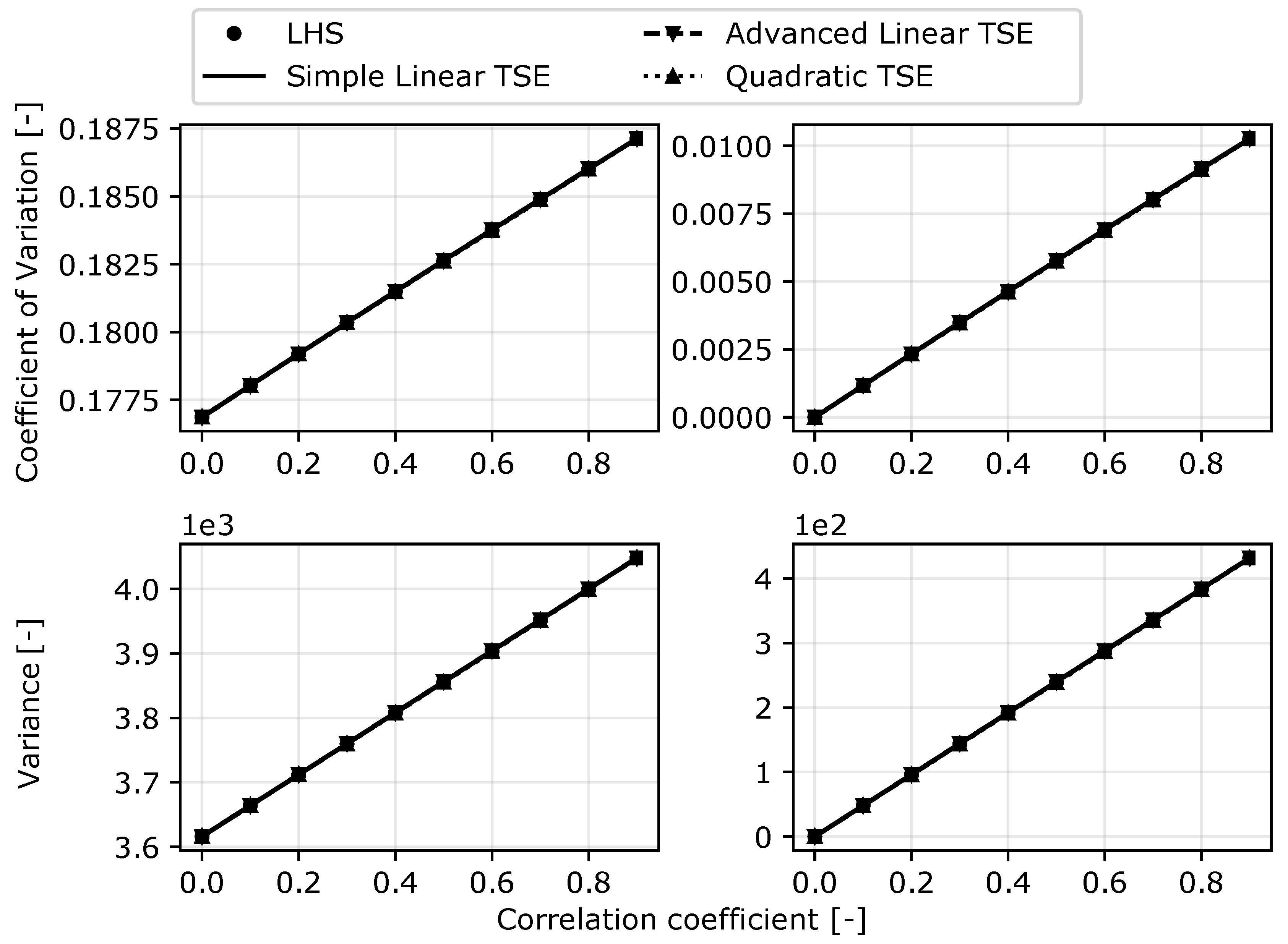
3.3. Example 1: Simple Linear Model

The very first example represents the entire methodology. It is a simple linear model R = r ( X ) = X 1 + X 2 . The selected realizations generated by Latin Hypercube Sampling, which illustrate the uniform cover of the design domain, together with iso-lines of joint probability density of random vector in uncorrelated and correlated space (Gaussian copula parametrized by the correlation coefficient ρ = 0.8 ) are depicted in Figure 2. A reference solution based on a sample with n s i m = 10 5 is calculated for all examples.
In this case, all the presented differencing schemes led to the exact solution, as can be seen in Figure 3, since a linear approximation fits the original model. For the sake of clarity, the figures in this section show estimation of CoV (top) and variance (bottom) as well, since CoV takes the estimation of mean value into account. The graphs in the right column represent CoV or variance for correlated variables with subtracted uncorrelated values, which represent pure influence of correlation estimated by the presented methods.

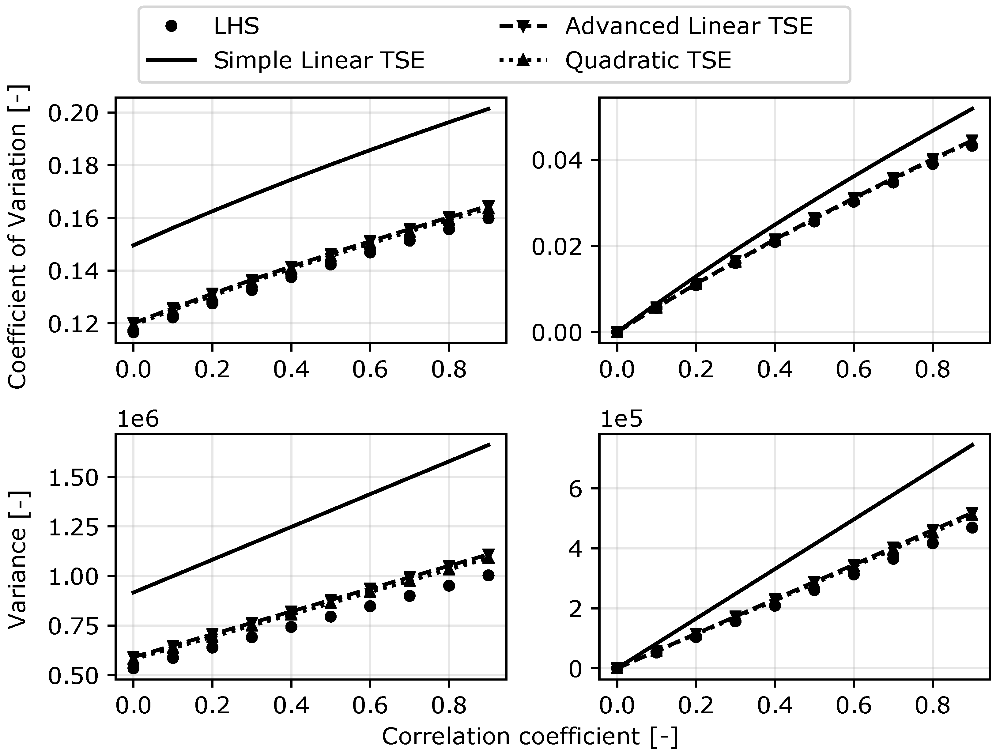
3.4. Example 2: Linear Model with Interactions

The second example is focused on the comparison of the first-order and the second-order Taylor series expansion. The first and the second level of approximation use the first-order Taylor expansion; thus, they are not recommended for mathematical models with significant interaction terms, since there are no mixed derivatives in the approximation, and the influence of the interaction is therefore underestimated. The quadratic TSE is the most computationally demanding and the only one reflecting the interaction terms. For the demonstration of this characteristic, the following adaptation of the previous simple mathematical model is assumed:
R = r ( X ) = X 1 + X 2 + 5 X 1 X 2
The obtained results are depicted in Figure 4 in the same manner as in the previous example. The estimated mean value for the uncorrelated input random variable was accurate ( μ R = 260 ). However, using only linear terms of Taylor expansion led to an identical mean value independent of the correlation among input variables. Therefore, the results of CoV are affected by this characteristic, and all methods seem comparable. The accuracy of the used approximations can be clearly seen on the estimation of variance, where the first two levels of an approximation led to identical results, with the error increasing together with the correlation between input random variables. Of course, the obtained results are exact only if the third-level approximation (quadratic Taylor expansion) is used for the estimation of variance, since Hessian of this function is not equal to the zero matrix 0 . As can be seen, neglecting an interaction among random variables by the first-order Taylor expansion may lead to a significant error in the estimation of statistical moments even for simple linear functions; thus, an analyst should carefully choose the level of approximation in industrial applications considering the nature of the studied physical system.

3.5. Example 3: Approximation of Industrial Example

The third example is motivated by the industrial applications in civil engineering often represented by non-linear finite element models—typically ultimate resistance given by the peak of the load-deflection curve of concrete structural element. The behavior of such a physical system is often monotone with a slightly non-linear progress. A typical function solved by FEM can be found, for example, in [9], and due to the computational demands of FEM, its shape was replicated by the following artificial function:
R = r ( X ) = X 1 X 2 X 1 2 X 2 2 30 X 1 30 X 2 200
The exact mean value estimated by LHS was μ R = 6264 and by Taylor series E R T = 6400 , which leads to the difference between the estimation of CoV and variance depicted in Figure 5. However, the estimation of variance and CoV by linear TSE with advanced differencing together with quadratic TSE was accurate. On the other hand, linear Taylor expansion with simple one-sided backward differencing showed a significant error in estimation for all correlation coefficients. The results on the right-hand side of Figure 5 represent the pure influence of correlation, and as can be seen, the slope of the curve estimated by simple linear TSE was significantly different. Thus, this method is not able to correctly identify the role of correlation.
From the previous examples, it is clear that simple linear Taylor expansion as proposed by Schlune et al. is suitable only for functions of uncorrelated variables, which is not a typical industrial problem. However, it is possible to start with simple differencing for uncorrelated problem and add n additional simulations in order to adapt an approximation for correlated variables.

3.6. Example 4: Non-Linear Function

The last example is created in order to show the limitations of all the presented methods with increasing non-linearity of the original mathematical model. The following function has a similar shape as the model in the previous example; however, it is significantly more non-linear:
R = r ( X ) = X 1 X 2 c o s π X 1 200 c o s π X 2 2000
The estimated mean value by TSE for the uncorrelated case was E R T = 8650 , and the exact value estimated by LHS was μ R = 8468 . Variance and CoV of R estimated by the presented methods are summarized in Figure 6. As can be expected, with higher non-linearity of mathematical models, it was not suitable anymore to use TSE of lower orders as an approximation of the original model. Since computational requirements of higher-order Taylor series expansions are comparable to the commonly known surrogate models, and the estimation of statistical moments is inefficient, one should prefer more advanced surrogate models (e.g., Polynomial Chaos Expansion or Kriging) together with standard statistical methods.
Specifically in this example, the worst results were obtained by the linear TSE with simple differencing, which represents a poor approximation of the original function; thus, the estimation of variance was not satisfied as well. Similarly, a poor accuracy of the estimated influence of correlation can be clearly seen from the different trends of the curves in the column on the right-hand side in Figure 6. However, since there is no significant interaction between the input random variables, the results obtained by linear Taylor series with advanced differencing were almost identical to the more computationally demanding quadratic Taylor series, which might be a crucial advantage in high-dimensional industrial applications solved by FEM.

4. Discussion

The TSE represents a powerful and accurate technique with a strong mathematical background. Unfortunately, it is usually truncated to linear terms in engineering applications, which may generally lead to poor results in the case of non-linear functions and correlated random input variables. Although Schlune et al. proposed the ECoV method based on linear TSE with a simple asymmetric differencing, there are no studies on its limitations and possible generalizations, although TSE is a highly modifiable technique via differencing schemes and a truncation order of an approximation. Therefore, it was necessary to propose different variations of TSE for specific problems and create the novel methodology of three levels of TSE. The proposed methodology was applied on several analytical examples in order to show the limitations of each level. The variations of TSE were proposed with attention to the reduction of computational cost as much as possible, since derivations are computed by finite differencing of FEM in industrial applications. Therefore, each additional level of the methodology works with the information previously obtained from calculations of the original mathematical model; thus, an approximation can be sequentially made more accurate by calculating several additional simulations and combining them with the previous results used in the asymmetric differencing scheme of lower levels of the proposed methodology.
It can be seen from the presented results, that linear TSE fails in the case of significantly non-linear functions (the last example) and functions with important interaction terms (the second example). In such cases, it is necessary to use quadratic TSE (3rd level of proposed methodology) as an approximation. Moreover, the main motivation of this paper is dealing with correlation among random input variables, which has not been investigated yet in the context of ECoV methods. It is clear from the presented examples that the linear TSE with simple differencing (1st level of the proposed methodology) is not suitable for functions of correlated variables. However, once the differencing scheme according to Equation (9) is used in combination with linear TSE (2nd level of the proposed methodology), its accuracy is significantly improved. Thus, if there is not a strong interaction among input random variables, it is not necessary to use quadratic TSE (3rd level of the proposed methodology), which leads to additional computational requirements.
From the point of view of computational costs, it is possible to add higher terms of Taylor series, but it significantly increases the number of derivatives. Therefore, TSE above the second order is inefficient, and advanced surrogate models such as PCE, Krigging, or ANN should be used. On the other hand, a better accuracy of estimation of CoV and variance can be reached by the improved asymmetric differencing scheme as proposed in this paper. Computational requirements are slightly increased from n + 1 , for the traditional scheme according to Equation (3), to 2 n + 1 for the proposed scheme according to Equation (9). It is obvious that variance estimation using Equation (9) is significantly improved in comparison to the traditional differencing scheme represented by Equation (3). However, the main advantage of the proposed method is the accuracy of variance estimation in the case of correlated random variables. It is obvious that there is a difference between the curves representing an increment of variance due to correlation (second part of Equation (8)) estimated by both approaches. The difference between both differencing schemes is proportional to a correlation among input random variables; thus, special attention should be given to functions with high correlation among input random variables.
Generally, the proposed methodology proved to be well-suited for typical industrial mathematical models in civil engineering. Moreover, the paper shows the influence of different variants of TSE and level of statistical correlation on estimated CoV, which is a base for semi-probabilistic approaches to determine design value in civil engineering. Such influence can be significant, for more basic random variables certainly amplified, which will be studied on practical examples represented by non-linear finite element models of structures in further research, and the obtained results will be compared to standard normative approaches as PSF and global safety factor method [24] designed specifically for civil engineering.

5. Conclusions

The non-linearity of functions and statistical correlation of input random variables represent crucial aspects in estimating statistical moments of industrial mathematical models. Unfortunately, the accuracy of standard existing methods is not satisfying for such models. Therefore, this paper presents a novel methodology to estimate the coefficient of variation for functions of correlated input random variables. Since mathematical models in civil engineering are often functions of input correlated random variables, it is necessary to develop new and efficient methods based on a semi-probabilistic approach widely accepted for the design and assessment of structures satisfying given safety requirements. Therefore, the methodology of three levels of increasing complexity, accuracy, and computational cost based on Taylor series expansion is proposed and described. The methodology consists of three advanced differencing schemes adapted for civil engineering by step size parameter. The differencing schemes are based on the asymmetric quotient, which is typical for engineering applications, where one is interested in extreme structural behavior leading to failure. The proposed methodology is applied to four analytical examples, and the results are compared to reference solutions obtained by Latin Hypercube Sampling. The analytical examples are constructed in order to show the efficiency and limitations of each differencing scheme: simple linear function, linear function with strong interaction terms, and finally two non-linear functions. From the obtained results, extensively discussed in the previous section, it is clear that it is necessary to choose advanced asymmetric differencing schemes in the cases of correlated input random variables or increase the truncation order of Taylor series expansion. It was shown that its accuracy is significantly higher in comparison to the simple linear TSE (in absolute values but also in a relative trend of influence of correlation). The slight increment of computational demands of the proposed differencing schemes is a significant advantage in comparison to Taylor series of a higher order, where it is necessary to numerically evaluate a large number of additional derivatives. However, it was shown that quadratic TSE is necessary for mathematical models with strong interaction terms.

Author Contributions

Methodology, L.N.; validation, L.N.; formal analysis, L.N.; writing—original draft preparation, L.N.; writing—review and editing, D.N. and L.N; visualization, L.N.; supervision, D.N.; funding acquisition, D.N. All authors have read and agreed to the published version of the manuscript.

Funding

This research was funded by by Czech Science Foundation under project No. 18-13212S and the support provided by the Czech Ministry of Education, Youth and Sports under project No. FAST-J-20-6417. The first author is Brno Ph.D. Talent Scholarship Holder—Funded by the Brno City Municipality.

Conflicts of Interest

The authors declare no conflict of interest.

References

  1. Cornell, C.A. A probability based structural code. J. Am. Concr. Inst. 1969, 66, 974–985. [Google Scholar]
  2. Comité Européen de Normalisation (CEN). EN 1990: Eurocode: Basis of Structural Design; Comité Européen de Normalisation: Brussels, Belgium, 2002. [Google Scholar]
  3. Hasofer, A.M.; Lind, N.C. Exact and Invariant Second-moment Code Format. J. Eng. Mech. Div. 1974, 100, 111–121. [Google Scholar]
  4. Rosenblatt, M. Remarks on a multivariate transformation. Ann. Math. Stat. 1952, 23, 470–472. [Google Scholar] [CrossRef]
  5. Pimentel, M.; Brühwiler, E.; Figueiras, J. Safety examination of existing concrete structures using the global resistance safety factor concept. Eng. Struct. 2014, 70, 130–143. [Google Scholar] [CrossRef]
  6. Cervenka, V. Reliability-based non-linear analysis according to fib Model Code 2010. Struct. Concr. 2013, 14, 19–28. [Google Scholar] [CrossRef]
  7. Val, D.; Bljuger, F.; Yankelevsky, D. Reliability evaluation in nonlinear analysis of reinforced concrete structures. Struct. Saf. 1997, 19, 203–217. [Google Scholar] [CrossRef]
  8. Cervenka, V. Global Safety Format for Nonlinear Calculation of Reinforced Concrete. Beton Und Stahlbetonbau 2008, 103, 37–42. [Google Scholar] [CrossRef]
  9. Schlune, H.; Plos, M.; Gylltoft, K. Safety formats for nonlinear analysis tested on concrete beams subjected to shear forces and bending moments. Eng. Struct. 2011, 33, 2350–2356. [Google Scholar] [CrossRef]
  10. Bertagnoli, G.; Giordano, L.M.; Mancini, G.F. Safety format for the nonlinear analysis of concrete structures. Studi e Ricerche- Politecnico di Milano. Scuola di Specializzazione in Costruzioni in Cemento Armato 2004, 25, 31–56. [Google Scholar]
  11. McKay, M.D. Latin Hypercube Sampling as a Tool in Uncertainty Analysis of Computer Models. In Proceedings of the 24th Conference on Winter Simulation, Arlington, VA, USA, 13–16 December 1992; pp. 557–564. [Google Scholar]
  12. Iman, R.L.; Conover, W. Small sample sensitivity analysis techniques for computer models with an application to risk assessment. Commun. Stat. Theory Methods 1980, 9, 1749–1842. [Google Scholar] [CrossRef]
  13. Sudret, B. Global sensitivity analysis using polynomial chaos expansions. Reliab. Eng. Syst. Saf. 2008, 93, 964–979. [Google Scholar] [CrossRef]
  14. Blatman, G.; Sudret, B. An adaptive algorithm to build up sparse polynomial chaos expansions for stochastic finite element analysis. Probabilistic Eng. Mech. 2010, 25, 183–197. [Google Scholar] [CrossRef]
  15. Echard, B.; Gayton, N.; Lemaire, M. AK-MCS: An active learning reliability method combining Kriging and Monte Carlo Simulation. Struct. Saf. 2011, 33, 145–154. [Google Scholar] [CrossRef]
  16. Lehky, D.; Somodikova, M. Reliability calculation of time-consuming problems using a small-sample artificial neural network-based response surface method. Neural Comput. Appl. 2016, 28, 1249–1263. [Google Scholar] [CrossRef]
  17. Melchers, R.E.; Beck, A.T. Second-Moment and Transformation Methods. In Structural Reliability Analysis and Prediction; John Wiley & Sons, Ltd.: Hoboken, NJ, USA, 2017; Chapter 4; pp. 95–130. [Google Scholar] [CrossRef]
  18. Paudel, A.; Thapa, M.; Gupta, S.; Mulani, S.B.; Walters, R.W. Higher-Order Taylor Series Expansion with Efficient Sensitivity Estimation for Uncertainty Analysis. In AIAA Aviation 2020 Forum; American Institute of Aeronautics and Astronautics: Reston, VA, USA, 2020. [Google Scholar]
  19. Sykora, M.; Cervenka, J.; Cervenka, V.; Mlcoch, J.; Novak, D.; Novak, L. Pilot comparison of safety formats for reliability assessment of RC structures. In Proceedings of the fib Symposium 2019: Concrete—Innovations in Materials, Design and Structures, Kraków, Poland, 27–29 May 2019; pp. 2076–2083. [Google Scholar]
  20. Novák, L.; Novák, D.; Pukl, R. Probabilistic and semi-probabilistic design of large concrete beams failing in shear. In Advances in Engineering Materials, Structures and Systems: Innovations, Mechanics and Applications; Taylor and Francis Group CRC Press: London, UK, 2019. [Google Scholar]
  21. Novák, D.; Novák, L.; Slowik, O.; Strauss, A. Prestressed concrete roof girders: Part III—Semi-probabilistic design. In Proceedings of the Sixth International Symposium on Life-Cycle Civil Engineering (IALCCE 2018), Ghent, Belgium, 28–31 October 2018; pp. 510–517. [Google Scholar]
  22. Lebrun, R.; Dutfoy, A. An innovating analysis of the Nataf transformation from the copula viewpoint. Probabilistic Eng. Mech. 2009, 24, 312–320. [Google Scholar] [CrossRef]
  23. Lebrun, R.; Dutfoy, A. Do Rosenblatt and Nataf isoprobabilistic transformations really differ? Probabilistic Eng. Mech. 2009, 24, 577–584. [Google Scholar] [CrossRef]
  24. Comité Européen de Normalisation (CEN). EN 1992: Eurocode 2: Design of Concrete Structures; Comité Européen de Normalisation: Brussels, Belgium, 2004. [Google Scholar]
Figure 1. Proposed methodology composed of the three levels of Taylor series expansion (TSE) approximation using asymmetric differencing schemes adapted for civil engineering. Iso-lines of bivariate standard Gaussian probability distribution are represented by dotted circles.
Symmetry 12 01379 g001
Figure 2. Realizations (red dots) generated by Latin Hypercube Sampling (LHS) and iso-lines of joint probability density of input random vector in uncorrelated (left) and correlated (right) space.
Symmetry 12 01379 g002
Figure 3. Estimation of coefficient of variance (CoV) (top) and variance (bottom) of the first example by the presented methods.
Symmetry 12 01379 g003
Figure 4. Estimation of CoV (top) and variance (bottom) of the second example by the presented methods.
Symmetry 12 01379 g004
Figure 5. Estimation of CoV (top) and variance (bottom) of the third example by the presented methods.
Symmetry 12 01379 g005
Figure 6. Estimation of CoV (top) and variance (bottom) of the fourth example by the presented methods.
Symmetry 12 01379 g006

