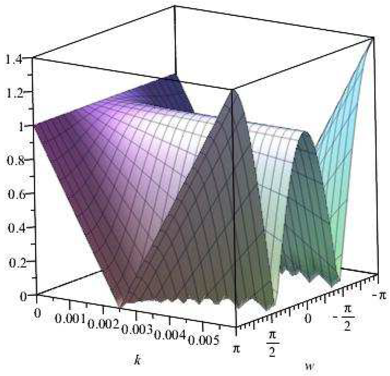
Figure 1.
Plot of vs. k vs. for .
Figure 1.
Plot of vs. k vs. for .
Figure 2.
Plot of vs. k vs. for .
Figure 2.
Plot of vs. k vs. for .
Figure 3.
Plot of vs. k vs. for .
Figure 3.
Plot of vs. k vs. for .
Figure 4.
Plot of vs. k vs. for .
Figure 4.
Plot of vs. k vs. for .
Figure 5.
Plot of vs. k vs. for .
Figure 5.
Plot of vs. k vs. for .
Figure 6.
Plot of vs. k vs. for .
Figure 6.
Plot of vs. k vs. for .
Figure 7.
Plot of vs. k vs. for .
Figure 7.
Plot of vs. k vs. for .
Figure 8.
Plot of vs. k vs. for .
Figure 8.
Plot of vs. k vs. for .
Figure 9.
Plot of vs. k vs. for .
Figure 9.
Plot of vs. k vs. for .
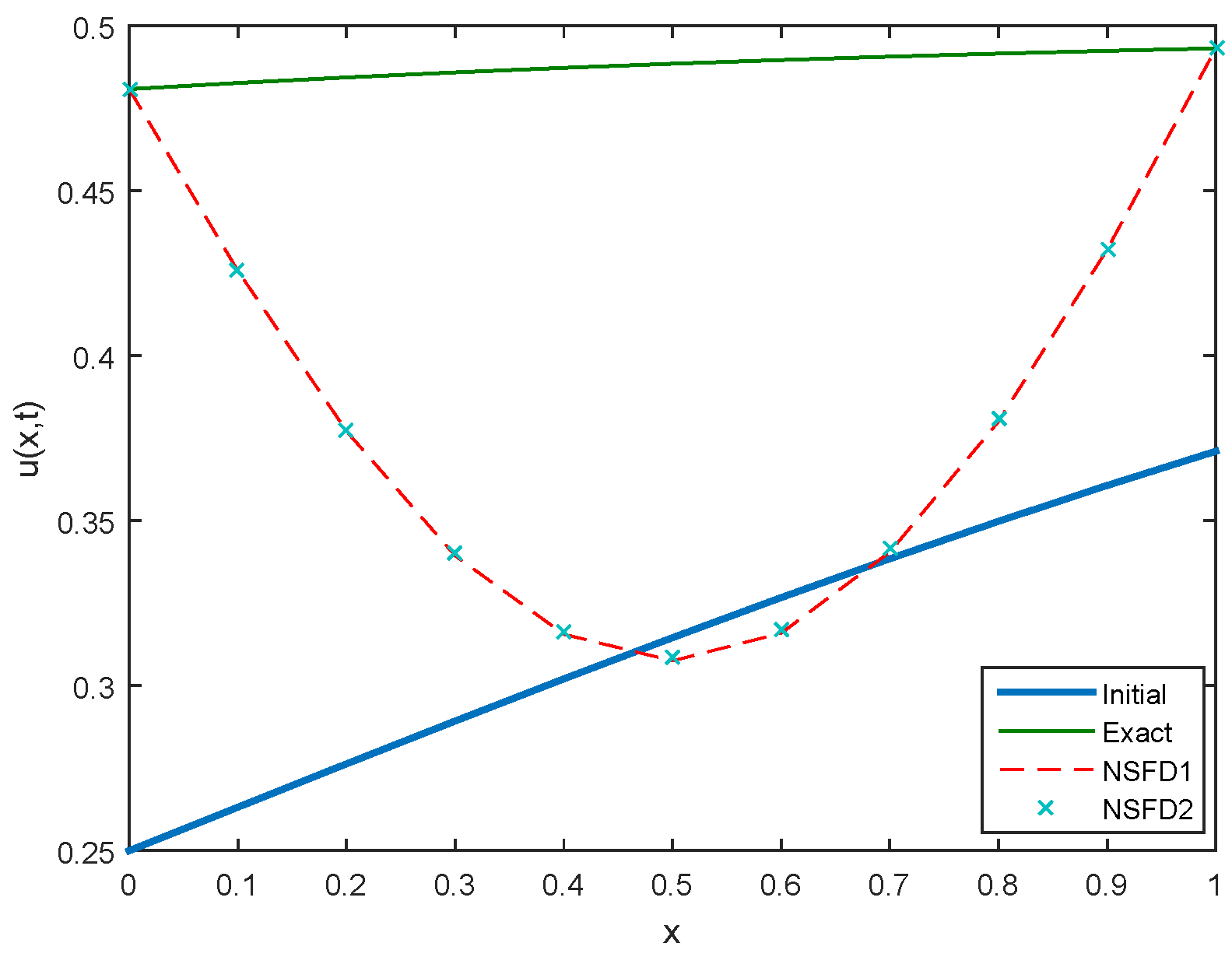
Figure 10.
Comparison between Initial, Exact, NSFD1 and NSFD2 profiles for Case 1 at .
Figure 10.
Comparison between Initial, Exact, NSFD1 and NSFD2 profiles for Case 1 at .
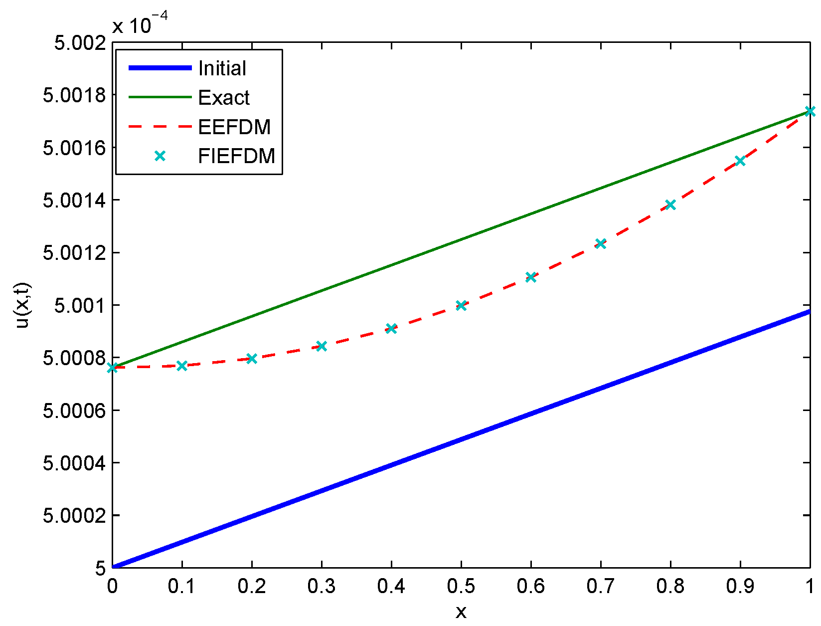
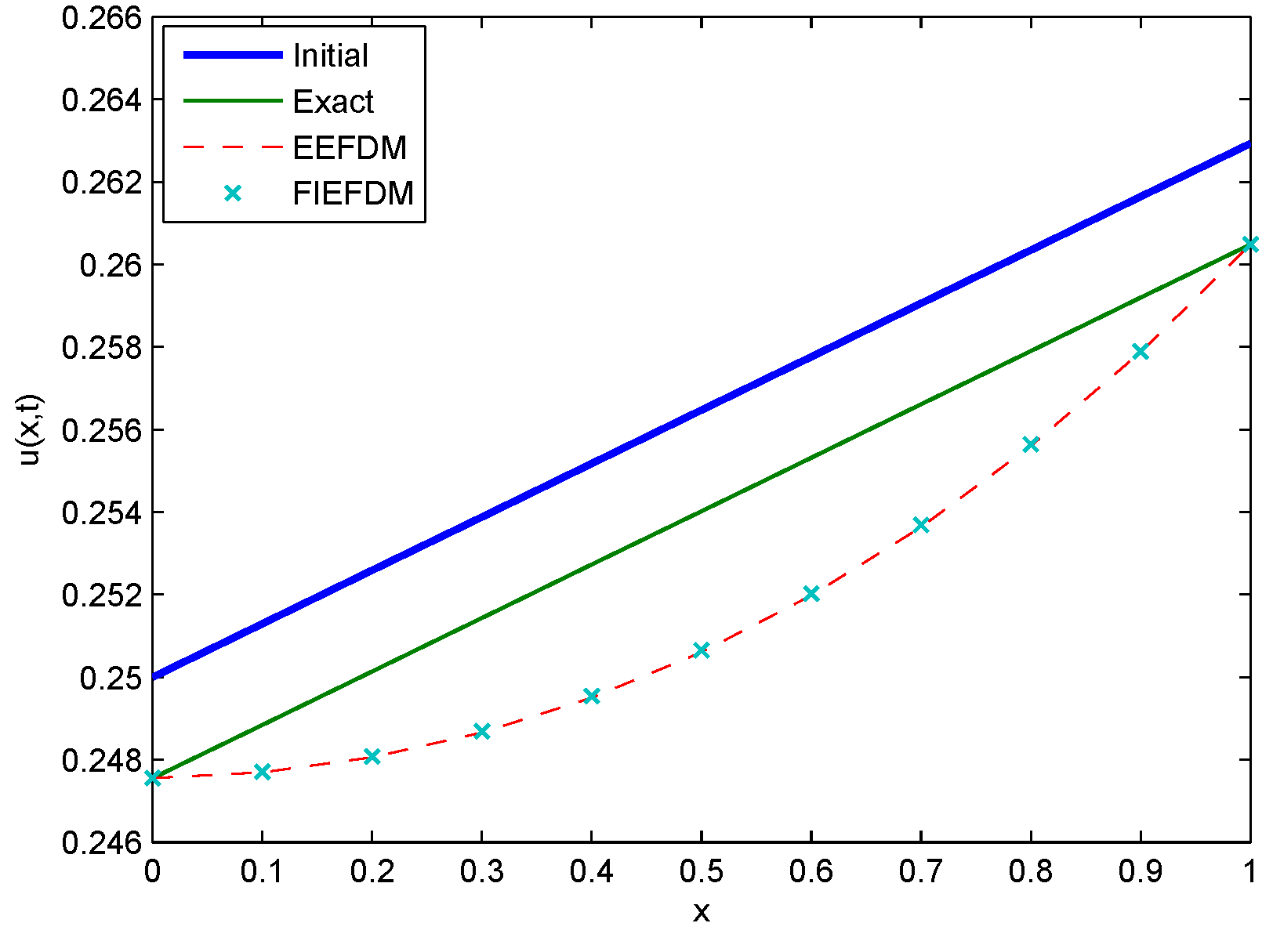
Figure 11.
Comparison between Initial, Exact, EEFDM and FIEFDM profiles for Case 1 at .
Figure 11.
Comparison between Initial, Exact, EEFDM and FIEFDM profiles for Case 1 at .
Figure 12.
Comparison between Initial, Exact, NSFD1 and NSFD2 profiles for Case 2 at .
Figure 12.
Comparison between Initial, Exact, NSFD1 and NSFD2 profiles for Case 2 at .
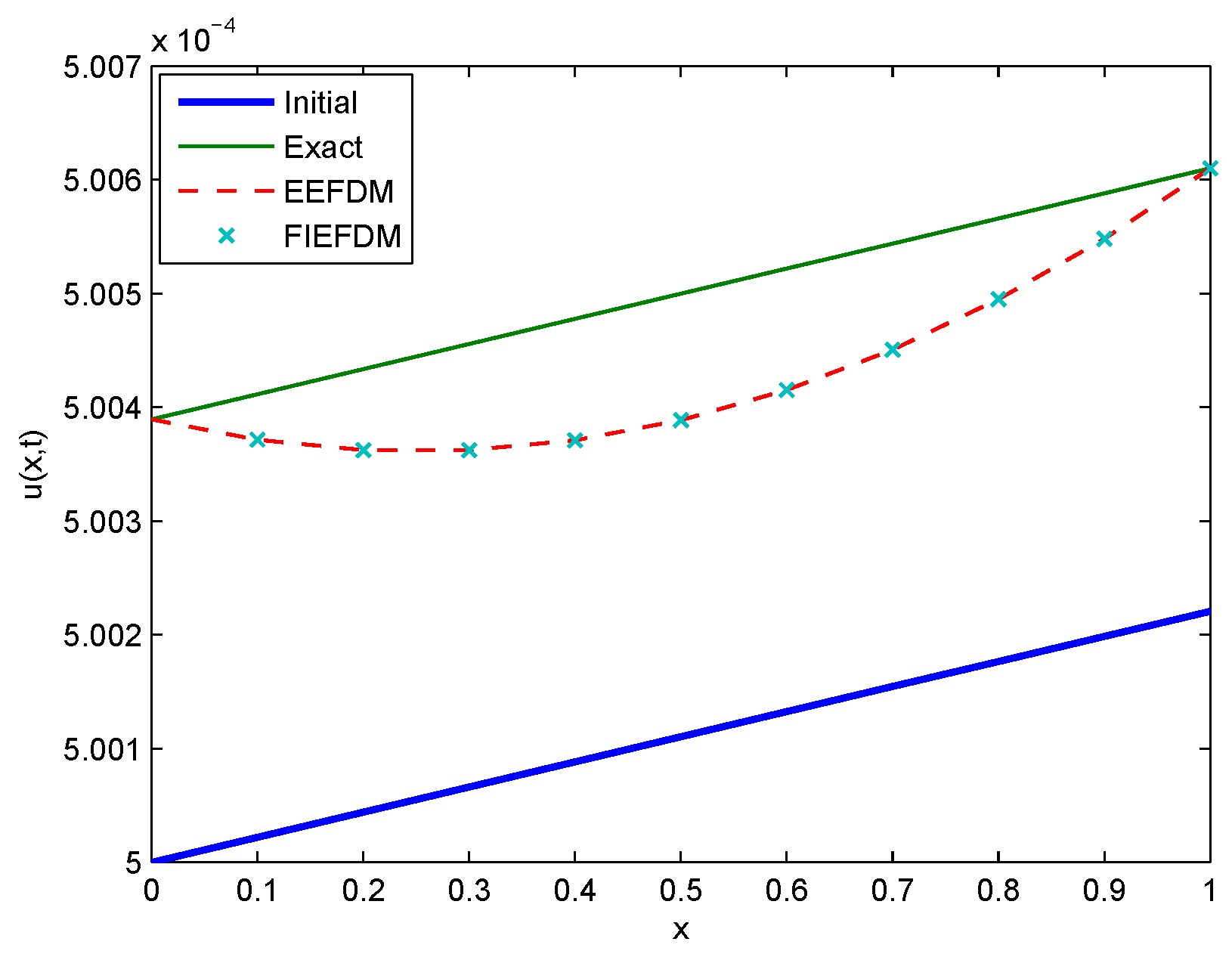
Figure 13.
Comparison between Initial, Exact, EEFDM and FIEFDM profiles for Case 2 at .
Figure 13.
Comparison between Initial, Exact, EEFDM and FIEFDM profiles for Case 2 at .
Figure 14.
Comparison between Initial, Exact, NSFD1 and NSFD2 profiles for Case 3 at .
Figure 14.
Comparison between Initial, Exact, NSFD1 and NSFD2 profiles for Case 3 at .
Figure 15.
Comparison between Initial, Exact, EEFDM and FIEFDM profiles for Case 3 at .
Figure 15.
Comparison between Initial, Exact, EEFDM and FIEFDM profiles for Case 3 at .
Figure 16.
Comparison between Initial, Exact, NSFD1 and NSFD2 profiles for Case 4 at .
Figure 16.
Comparison between Initial, Exact, NSFD1 and NSFD2 profiles for Case 4 at .
Figure 17.
Comparison between Initial, Exact, EEFDM and FIEFDM profiles for Case 4 at .
Figure 17.
Comparison between Initial, Exact, EEFDM and FIEFDM profiles for Case 4 at .
Figure 18.
Comparison between Initial, Exact, NSFD1 and NSFD2 profiles for Case 5 at .
Figure 18.
Comparison between Initial, Exact, NSFD1 and NSFD2 profiles for Case 5 at .
Figure 19.
Comparison between Initial, Exact, EEFDM and FIEFDM profiles for Case 5 at .
Figure 19.
Comparison between Initial, Exact, EEFDM and FIEFDM profiles for Case 5 at .
Figure 20.
Comparison between Initial, Exact, NSFD1 and NSFD2 profiles for Case 6 at .
Figure 20.
Comparison between Initial, Exact, NSFD1 and NSFD2 profiles for Case 6 at .
Figure 21.
Comparison between Initial, Exact, EEFDM and FIEFDM profiles for Case 6 at .
Figure 21.
Comparison between Initial, Exact, EEFDM and FIEFDM profiles for Case 6 at .
Figure 22.
Comparison between Initial, Exact, NSFD1 and NSFD2 profiles for Case 7 at .
Figure 22.
Comparison between Initial, Exact, NSFD1 and NSFD2 profiles for Case 7 at .
Figure 23.
Comparison between Initial, Exact, EEFDM and FIEFDM profiles for Case 7 at .
Figure 23.
Comparison between Initial, Exact, EEFDM and FIEFDM profiles for Case 7 at .
Figure 24.
Comparison between Initial, Exact, NSFD1 and NSFD2 profiles for Case 8 at .
Figure 24.
Comparison between Initial, Exact, NSFD1 and NSFD2 profiles for Case 8 at .
Figure 25.
Comparison between Initial, Exact, EEFDM and FIEFDM profiles for Case 8 at .
Figure 25.
Comparison between Initial, Exact, EEFDM and FIEFDM profiles for Case 8 at .
Figure 26.
Comparison between Initial, Exact, NSFD1 and NSFD2 profiles for Case 9 at .
Figure 26.
Comparison between Initial, Exact, NSFD1 and NSFD2 profiles for Case 9 at .
Figure 27.
Comparison between Initial, Exact, EEFDM and FIEFDM profiles for Case 9 at .
Figure 27.
Comparison between Initial, Exact, EEFDM and FIEFDM profiles for Case 9 at .
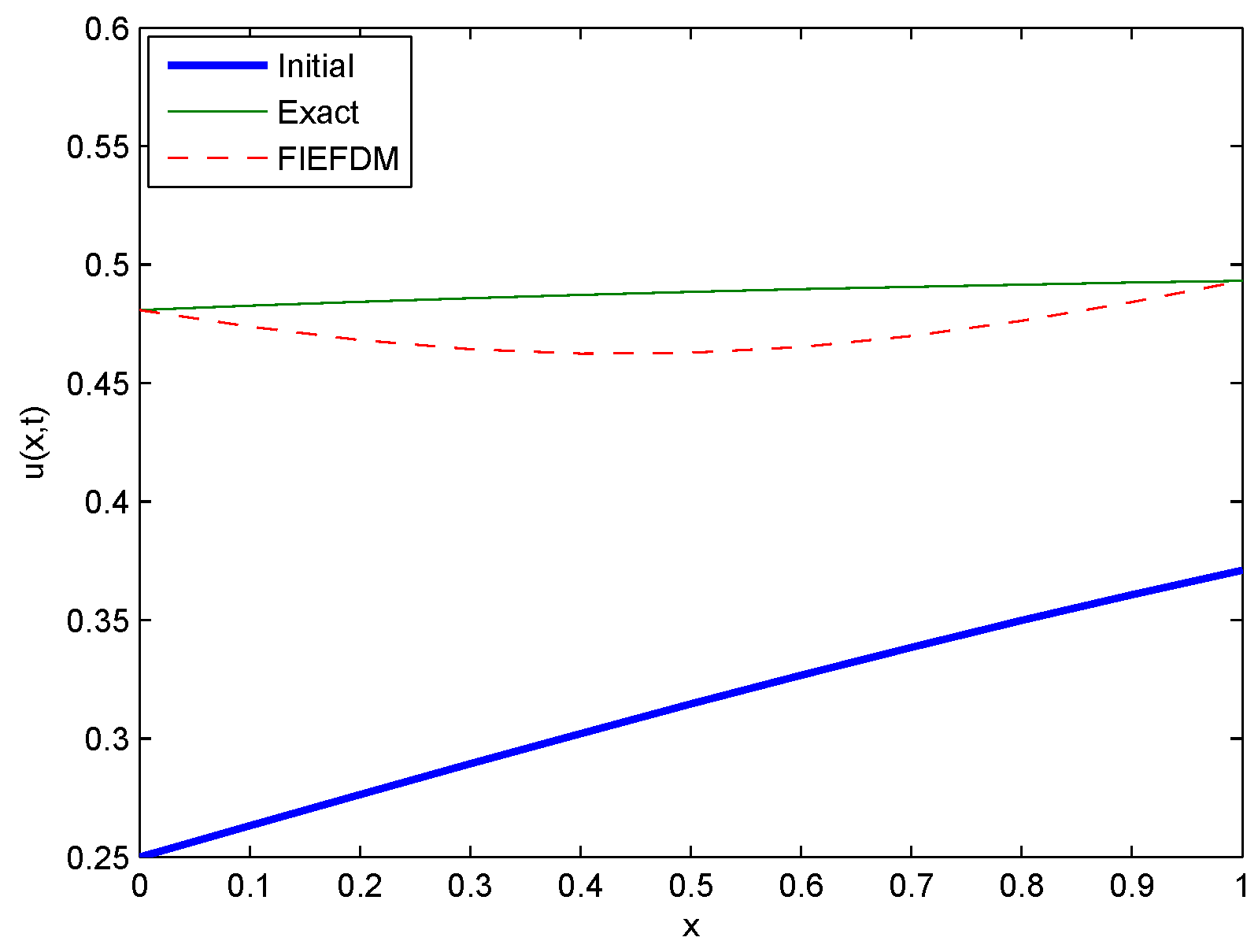
Figure 28.
Comparison between Initial, Exact and FIEFDM profiles for Case 10 at .
Figure 28.
Comparison between Initial, Exact and FIEFDM profiles for Case 10 at .
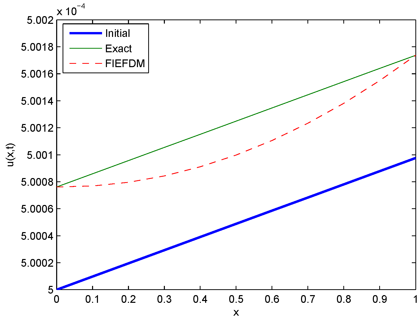
Figure 29.
Comparison between Initial, Exact and FIEFDM profiles for Case 11 at .
Figure 29.
Comparison between Initial, Exact and FIEFDM profiles for Case 11 at .
Table 1.
Range of values of k for stability of EEFDM with .
Table 1.
Range of values of k for stability of EEFDM with .
| Cases | Parameter Values | Condition for Stability |
|---|
| 1 | | |
| 2 | | |
| 3 | | |
| 4 | | |
| 5 | | |
| 6 | | |
| 7 | | |
| 8 | | |
| 9 | | |
Table 2.
A comparison between the exact and the numerical solutions at some values of x.
Table 2.
A comparison between the exact and the numerical solutions at some values of x.
| t | x | Exact | NSFD1 | NSFD2 | EEFDM | FIEFDM |
|---|
| 1 | | | | | | |
| | | | | | | |
| | | | | | | |
| 10 | | | | | | |
| | | | | | | |
| | | | | | | |
Table 3.
The absolute errors at some values of x for each of the numerical schemes.
Table 3.
The absolute errors at some values of x for each of the numerical schemes.
| t | x | NSFD1 | NSFD2 | EEFDM | FIEFDM |
|---|
| 1 | | | | | |
| | | | | | |
| | | | | | |
| 10 | | | | | |
| | | | | | |
| | | | | | |
Table 4.
The relative errors at some values of x for each of the numerical schemes.
Table 4.
The relative errors at some values of x for each of the numerical schemes.
| t | x | NSFD1 | NSFD2 | EEFDM | FIEFDM |
|---|
| 1 | | | | | |
| | | | | | |
| | | | | | |
| 10 | | | | | |
| | | | | | |
| | | | | | |
Table 5.
and error norms with CPU time taken for the four numerical methods.
Table 5.
and error norms with CPU time taken for the four numerical methods.
| t | Schemes | | | CPU Time |
|---|
| 1 | NSFD1 | | | |
| | NSFD2 | | | |
| | EEFDM | | | |
| | FIEFDM | | | |
| 10 | NSFD1 | | | |
| | NSFD2 | | | |
| | EEFDM | | | |
| | FIEFDM | | | |
Table 6.
A comparison between the exact and the numerical solutions at some values of x.
Table 6.
A comparison between the exact and the numerical solutions at some values of x.
| t | x | Exact | NSFD1 | NSFD2 | EEFDM | FIEFDM |
|---|
| 1 | | | | | | |
| | | | | | | |
| | | | | | | |
| 10 | | | | | | |
| | | | | | | |
| | | | | | | |
Table 7.
The absolute errors at some values of x for each of the numerical schemes.
Table 7.
The absolute errors at some values of x for each of the numerical schemes.
| t | x | NSFD1 | NSFD2 | EEFDM | FIEFDM |
|---|
| 1 | | | | | |
| | | | | | |
| | | | | | |
| 10 | | | | | |
| | | | | | |
| | | | | | |
Table 8.
The relative errors at some values of x for each of the numerical schemes.
Table 8.
The relative errors at some values of x for each of the numerical schemes.
| t | x | NSFD1 | NSFD2 | EEFDM | FIEFDM |
|---|
| 1 | | | | | |
| | | | | | |
| | | | | | |
| 10 | | | | | |
| | | | | | |
| | | | | | |
Table 9.
and error norms with CPU time taken for the four numerical methods.
Table 9.
and error norms with CPU time taken for the four numerical methods.
| t | Schemes | | | CPU Time (Sec) |
|---|
| 1 | NSFD1 | | | |
| | NSFD2 | | | |
| | EEFDM | | | |
| | FIEFDM | | | |
| 10 | NSFD1 | | | |
| | NSFD2 | | | |
| | EEFDM | | | |
| | FIEFDM | | | |
Table 10.
A comparison between the exact and the numerical solutions at some values of x.
Table 10.
A comparison between the exact and the numerical solutions at some values of x.
| t | x | Exact | NSFD1 | NSFD2 | EEFDM | FIEFDM |
|---|
| 1 | | | | | | |
| | | | | | | |
| | | | | | | |
| 10 | | | | | | |
| | | | | | | |
| | | | | | | |
Table 11.
The absolute errors at some values of x for each of the numerical schemes.
Table 11.
The absolute errors at some values of x for each of the numerical schemes.
| t | x | NSFD1 | NSFD2 | EEFDM | FIEFDM |
|---|
| 1 | | | | | |
| | | | | | |
| | | | | | |
| 10 | | | | | |
| | | | | | |
| | | | | | |
Table 12.
The relative errors at some values of x for each of the numerical schemes.
Table 12.
The relative errors at some values of x for each of the numerical schemes.
| t | x | NSFD1 | NSFD2 | EEFDM | FIEFDM |
|---|
| 1 | | | | | |
| | | | | | |
| | | | | | |
| 10 | | | | | |
| | | | | | |
| | | | | | |
Table 13.
and error norms with CPU time taken for the four numerical methods.
Table 13.
and error norms with CPU time taken for the four numerical methods.
| t | Schemes | | | CPU Time (Sec) |
|---|
| 1 | NSFD1 | | | |
| | NSFD2 | | | |
| | EEFDM | | | |
| | FIEFDM | | | |
| 10 | NSFD1 | | | |
| | NSFD2 | | | |
| | EEFDM | | | |
| | FIEFDM | | | |
Table 14.
A comparison between the exact and the numerical solutions at some values of x.
Table 14.
A comparison between the exact and the numerical solutions at some values of x.
| t | x | Exact | NSFD1 | NSFD2 | EEFDM | FIEFDM |
|---|
| 1 | | | | | | |
| | | | | | | |
| | | | | | | |
| 10 | | | | | | |
| | | | | | | |
| | | | | | | |
Table 15.
The absolute errors at some values of x for each of the numerical schemes.
Table 15.
The absolute errors at some values of x for each of the numerical schemes.
| t | x | NSFD1 | NSFD2 | EEFDM | FIEFDM |
|---|
| 1 | | | | | |
| | | | | | |
| | | | | | |
| 10 | | | | | |
| | | | | | |
| | | | | | |
Table 16.
The relative errors at some values of x for each of the numerical schemes.
Table 16.
The relative errors at some values of x for each of the numerical schemes.
| t | x | NSFD1 | NSFD2 | EEFDM | FIEFDM |
|---|
| 1 | | | | | |
| | | | | | |
| | | | | | |
| 10 | | | | | |
| | | | | | |
| | | | | | |
Table 17.
and error norms with CPU time taken for the four numerical methods.
Table 17.
and error norms with CPU time taken for the four numerical methods.
| t | Schemes | | | CPU Time (Sec) |
|---|
| 1 | NSFD1 | | | |
| | NSFD2 | | | |
| | EEFDM | | | |
| | FIEFDM | | | |
| 10 | NSFD1 | | | |
| | NSFD2 | | | |
| | EEFDM | | | |
| | FIEFDM | | | |
Table 18.
A comparison between the exact and the numerical solutions at some values of x.
Table 18.
A comparison between the exact and the numerical solutions at some values of x.
| t | x | Exact | NSFD1 | NSFD2 | EEFDM | FIEFDM |
|---|
| 1 | | | | | | |
| | | | | | | |
| | | | | | | |
| 10 | | | | | | |
| | | | | | | |
| | | | | | | |
Table 19.
The absolute errors at some values of x for each of the numerical schemes.
Table 19.
The absolute errors at some values of x for each of the numerical schemes.
| t | x | NSFD1 | NSFD2 | EEFDM | FIEFDM |
|---|
| 1 | | | | | |
| | | | | | |
| | | | | | |
| 10 | | | | | |
| | | | | | |
| | | | | | |
Table 20.
The relative errors at some values of x for each of the numerical schemes.
Table 20.
The relative errors at some values of x for each of the numerical schemes.
| t | x | NSFD1 | NSFD2 | EEFDM | FIEFDM |
|---|
| 1 | | | | | |
| | | | | | |
| | | | | | |
| 10 | | | | | |
| | | | | | |
| | | | | | |
Table 21.
and error norms with CPU times for the four numerical methods.
Table 21.
and error norms with CPU times for the four numerical methods.
| t | Schemes | | | CPU Time (Sec) |
|---|
| 1 | NSFD1 | | | |
| | NSFD2 | | | |
| | EEFDM | | | |
| | FIEFDM | | | |
| 10 | NSFD1 | | | |
| | NSFD2 | | | |
| | EEFDM | | | |
| | FIEFDM | | | |
Table 22.
A comparison between the exact and the numerical solutions at some values of x.
Table 22.
A comparison between the exact and the numerical solutions at some values of x.
| t | x | Exact | NSFD1 | NSFD2 | EEFDM | FIEFDM |
|---|
| 1 | | | | | | |
| | | | | | | |
| | | | | | | |
| 10 | | | | | | |
| | | | | | | |
| | | | | | | |
Table 23.
The absolute errors at some values of x for each of the numerical schemes.
Table 23.
The absolute errors at some values of x for each of the numerical schemes.
| t | x | NSFD1 | NSFD2 | EEFDM | FIEFDM |
|---|
| 1 | | | | | |
| | | | | | |
| | | | | | |
| 10 | | | | | |
| | | | | | |
| | | | | | |
Table 24.
The relative errors at some values of x for each of the numerical schemes.
Table 24.
The relative errors at some values of x for each of the numerical schemes.
| t | x | NSFD1 | NSFD2 | EEFDM | FIEFDM |
|---|
| 1 | | | | | |
| | | | | | |
| | | | | | |
| 10 | | | | | |
| | | | | | |
| | | | | | |
Table 25.
and error norms with CPU times for the four numerical methods.
Table 25.
and error norms with CPU times for the four numerical methods.
| t | Schemes | | | CPU Time (Sec) |
|---|
| 1 | NSFD1 | | | |
| | NSFD2 | | | |
| | EEFDM | | | |
| | FIEFDM | | | |
| 10 | NSFD1 | | | |
| | NSFD2 | | | |
| | EEFDM | | | |
| | FIEFDM | | | |
Table 26.
A comparison between the exact and the numerical solutions at some values of x.
Table 26.
A comparison between the exact and the numerical solutions at some values of x.
| t | x | Exact | NSFD1 | NSFD2 | EEFDM | FIEFDM |
|---|
| 1 | | | | | | |
| | | | | | | |
| | | | | | | |
| 10 | | | | | | |
| | | | | | | |
| | | | | | | |
Table 27.
The absolute errors at some values of x for each of the numerical schemes.
Table 27.
The absolute errors at some values of x for each of the numerical schemes.
| t | x | NSFD1 | NSFD2 | EEFDM | FIEFDM |
|---|
| 1 | | | | | |
| | | | | | |
| | | | | | |
| 10 | | | | | |
| | | | | | |
| | | | | | |
Table 28.
The relative errors at some values of x for each of the numerical schemes.
Table 28.
The relative errors at some values of x for each of the numerical schemes.
| t | x | NSFD1 | NSFD2 | EEFDM | FIEFDM |
|---|
| 1 | | | | | |
| | | | | | |
| | | | | | |
| 10 | | | | | |
| | | | | | |
| | | | | | |
Table 29.
and error norms with CPU time taken for the four numerical methods.
Table 29.
and error norms with CPU time taken for the four numerical methods.
| t | Schemes | | | CPU Time (Sec) |
|---|
| 1 | NSFD1 | | | |
| | NSFD2 | | | |
| | EEFDM | | | |
| | FIEFDM | | | |
| 10 | NSFD1 | | | |
| | NSFD2 | | | |
| | EEFDM | | | |
| | FIEFDM | | | |
Table 30.
A comparison between the exact and the numerical solutions at some values of x.
Table 30.
A comparison between the exact and the numerical solutions at some values of x.
| t | x | Exact | NSFD1 | NSFD2 | EEFDM | FIEFDM |
|---|
| 1 | | | | | | |
| | | | | | | |
| | | | | | | |
| 10 | | | | | | |
| | | | | | | |
| | | | | | | |
Table 31.
The absolute errors at some values of x for each of the numerical schemes.
Table 31.
The absolute errors at some values of x for each of the numerical schemes.
| t | x | NSFD1 | NSFD2 | EEFDM | FIEFDM |
|---|
| 1 | | | | | |
| | | | | | |
| | | | | | |
| 10 | | | | | |
| | | | | | |
| | | | | | |
Table 32.
The relative errors at some values of x for each of the numerical schemes.
Table 32.
The relative errors at some values of x for each of the numerical schemes.
| t | x | NSFD1 | NSFD2 | EEFDM | FIEFDM |
|---|
| 1 | | | | | |
| | | | | | |
| | | | | | |
| 10 | | | | | |
| | | | | | |
| | | | | | |
Table 33.
and error norms with CPU times for the four numerical methods.
Table 33.
and error norms with CPU times for the four numerical methods.
| t | Schemes | | | CPU Time (Sec) |
|---|
| 1 | NSFD1 | | | |
| | NSFD2 | | | |
| | EEFDM | | | |
| | FIEFDM | | | |
| 10 | NSFD1 | | | |
| | NSFD2 | | | |
| | EEFDM | | | |
| | FIEFDM | | | |
Table 34.
Absolute errors from four constructed schemes with the results of [
13,
14] for
.
Table 34.
Absolute errors from four constructed schemes with the results of [
13,
14] for
.
| t | x | NSFD1 | NSFD2 | EEFDM | FIEFDM | ADM | VIM |
|---|
| | | | | | | |
| | | | | | | | |
| | | | | | | | |
| | | | | | | |
| | | | | | | | |
| | | | | | | | |
| | | | | | | |
| | | | | | | | |
| | | | | | | | |
Table 35.
A comparison between the exact and numerical solutions with absolute and relative errors at some values of x.
Table 35.
A comparison between the exact and numerical solutions with absolute and relative errors at some values of x.
| t | x | Exact | FIEFDM | Absolute Error | Relative Error |
|---|
| 1 | | | | | |
| | | | | | |
| | | | | | |
| 10 | | | | | |
| | | | | | |
| | | | | | |
Table 36.
and error norms with CPU times for the FIEFDM.
Table 36.
and error norms with CPU times for the FIEFDM.
| t | | | CPU Time (Sec) |
|---|
| 1.0 | | | |
| 10.0 | | | |
Table 37.
A comparison between the exact and numerical solutions with absolute and relative errors at some values of x.
Table 37.
A comparison between the exact and numerical solutions with absolute and relative errors at some values of x.
| t | x | Exact | FIEFDM | Absolute Error | Relative Error |
|---|
| 1 | | | | | |
| | | | | | |
| | | | | | |
| 10 | | | | | |
| | | | | | |
| | | | | | |
Table 38.
and error norms with CPU times for the FIEFDM.
Table 38.
and error norms with CPU times for the FIEFDM.
| t | | | CPU Time (Sec) |
|---|
| 1.0 | | | |
| 10.0 | | | |


