Coordinated Control and Dynamic Optimal Dispatch of Islanded Microgrid System Based on GWO

Abstract

As an effective carrier of renewable distributed power sources, such as wind power and photovoltaics, microgrids have attracted increasing attention as the energy crisis becomes more serious. This paper focuses on the symmetry between the dynamic optimal dispatch and the coordinated control of islanded microgrid to determine the optimal system configuration that can reliably meet energy needs. In order to solve energy management problems, operating costs and environmental benefits, a novel methodology that combines dynamic optimal dispatch and Grey Wolf Optimizer (GWO) is developed in this study to obtain the best output of different system components. This is to minimize the total cost of microgrid power generation and reduce pollutant emissions. In addition, a comparison is carried out between GWO and Particle Swarm Optimization (PSO). Moreover, the comparison between system configurations in six different scenarios and the effectiveness of GWO in solving optimization problems are presented. Finally, the simulation results show that GWO is more effective than PSO in determining the optimization parameters and the utilization rate of renewable energy in different scenarios is up to 92.96%. The simulations and experimental results verify the successful performance of the research method proposed in this study.

1. Introduction

As the energy crisis becomes more serious, renewable distributed power sources, such as wind power and photovoltaics have gradually been developed, and microgrids are attracting further attention [1]. A microgrid is a small power generation and distribution system that integrates distributed power sources, energy storage devices, loads, and protection devices, and with the characteristics of flexible, reliable and safe power supply [2].

In order to use all kinds of energy reasonably and effectively, the microgrid energy scheduling meets certain constraints and load demands, and rationally dispatch energy and energy storage devices, which can effectively reduce operating costs and improve environmental benefits [3]. The energy dispatch of the microgrid is a key content in the related research problems of the microgrid. The factors considered in the dispatch model will affect the final dispatch result. Its purpose is to reasonably allocate the various loads under the premise of meeting the normal demand of all loads [4]. The output of the unit minimizes the total operating cost of the microgrid, thereby achieving the best economic benefits [5]. Dey et al. [6] studied the economic dispatch of a grid-connected renewable integrated microgrid system. Yuan et al. [7] proposed an energy management strategy based on hybrid prediction for the data interruption. Xin Li, et al. [8] considered that the microgrid environment/economic dispatch is a complex multi-objective optimization problem and reduced specific requirements for algorithm performance. Tiaan et al. [9] studied a multi-objective optimization model for multi-microgrid systems, which can not only minimize operating costs, but also reduce emissions.

Most of these papers use a static optimization scheduling model that aim to minimize the operation cost of the microgrid. Since the research on the economic optimal scheduling of the microgrid focuses on the operating economy after the system is built, the construction investment cost of the microgrid are not considered in most models, and the correlation between each time period is usually ignored. Each time period is independently optomised [10]. Compared with traditional power grids, the optimal dispatch of microgrids is more complicated, and traditional optimization methods cannot achieve optimal dispatch results. Various optimization methods based on artificial intelligence have the characteristics of fast convergence speed and not easy to fall into the local optimum. These optimization methods mainly include: Genetic Algorithm (GA) [11,12], PSO [13], and GWO [14]. However, GA and PSO also have their own disadvantages. The non-directional mutation of GA is its basic disadvantage. Likewise the convergence speed of PSO is not fast enough. In addition, the diversity of PSO is not enough, and it takes a long time to adjust the parameters in the optimization strategy. This paper uses PSO and GWO to compare and verify the effectiveness and accuracy of GWO in optimal scheduling. Naderi et al. [15] used fuzzy based hybrid PSO-DE to perform multi-objective economic emission dispatch on 10, 40 and 160 unit systems consider power loss, ramp rate, prohibited operating zones and valve point effects. In [16], a new multi-objective GWO for Optimal Reactive Power Dispatch (MORPD) is studied, which minimizes voltage deviation and active power loss (http://hainan.weather.com.cn/skjc/index.shtml).

Although a lot of work has been done in the above research on optimal dispatch of microgrid systems, none has studied dynamic optimal dispatch in conjunction with GWO. Instead, they use other intelligent algorithms to solve the optimization problem or study the static optimal dispatch of the microgrid. This paper proposes a new technology that combines dynamic optimal dispatch and GWO to achieve symmetry between the lowest operating cost of microgrid system and coordinated control of various devices. In addition, the proposed GWO is compared with the classic PSO to prove the effectiveness of the proposed method for dynamic optimal scheduling of microgrid systems. The comparison clearly shows that GWO has better performance, and has very fast convergence and balance in system optimization, which can avoid local optimization. The case study in this paper takes the Sanya region of China as an example. The region has 2534 h of sunshine throughout the year and has sufficient light.

The rest of this paper is organized as follows: The mathematical modeling of the microgrid components is elaborated in Section 2. The establishment of the objective function is described in Section 3. The constraints in the system are described in Section 4. In Section 5, the strategy of dynamic optimization scheduling for the system is outlined, and the GWO is introduced. Finally, the simulation results of the case study are presented and analyzed.

2. Mathematical Modeling

The basic structure of the microgrid is shown in Figure 1. The structure of the microgrid system includes wind power generation system (WT), photovoltaic power generation system (PV), energy storage system (ess), diesel generator (DG), and four power loads. Among them, as the micro power source of the main output unit in the microgrid, wind and solar power generation units use natural energy to generate electricity [16], which does not produce any pollutants but as natural resources, they also have their own limitations [17]. Restricted by natural conditions, randomness, volatility and intermittent characteristics have also become the inherent attributes and difficulties of clean energy power generation [18]. As an important coordination part of the system, the battery energy storage system is mainly used to coordinate the supply and demand balance of the microgrid, which plays a role in cutting peaks and filling valleys and smoothing fluctuations [19,20]. The backup power supply is used as a supplement to the microgrid power generation unit to ensure that some important loads in the microgrid system can be continuously and uninterrupted in the event of an emergency. Finally, each distributed unit in the microgrid is controlled by the microgrid energy management system to coordinate to form a unified system and maintain safe and stable operation.

2.1. Model of Wind Turbine

Wind power generation is one of the important power generation units in the microgrid. As the objective of this paper is to optimize the microgrid, it is also necessary to predict the active power output by the wind turbine. The rotation speed of the hub is related to the wind speed, so the analysis of modeling the output power of the wind turbine is essentially an accurate measurement of the wind speed of the wind turbine hub [21]. Considering the measurement of the wind speed of the fan hub, the cut-in wind speed V_ci, rated wind speed V_r, and cut-out wind speed V_co are often used. Three physical quantities are measured, and then the fan output power characteristic equation is obtained by curve fitting. All wind turbines have roughly the same wind speed power curve shape. Total extracted power from the wind turbines P_wt at any time can be calculated as follows [22]:

$$P_{wt}(v)=\{\begin{array}{c}0 , 0\le v\le v_{ci}\\ a·v^3-b·P_{wt-rate} , v_{ci}\le v\le v_r\\ P_{wt-rate} , v_r\le v\le v_{co}\end{array}$$

(1)

The constants a and b are given by the following equations [22]:

$$a=\frac{P_{wt-rate}}{v_r^3-v_{ci}^3} b=\frac{v_{ci}}{v_r^3-v_{ci}^3}$$

(2)

where a and b respectively represent the fitting coefficients of the WT output power, and P_wt−rate is the rated power of the WT. Generally, in the standard test case, the wind speed power characteristic curve of the wind turbine is drawn, and then the wind speed power expression shown in the above formula is obtained by curve fitting, but there are certain errors in the actual environment, so the standard test environment is correct the wind speed power characteristic curve obtained below.

2.2. Model of PV Array

PV power generation is one of the main power generation units in the microgrid system. In solving the problem of microgrid optimization and dispatch, it is necessary to accurately predict the power of photovoltaic power generation. Therefore, the output power of photovoltaic should consider solar radiation and temperature, the function is as follows [23]:

$$P_{pv}(t)=N_{pv}{P}_{rate-pv}\ast \frac{S}{S_{ref}}\ast [1+K_t(T_c-T_{ref})]$$

(3)

where P_pv is the output power of PV arrays, N_pv is numbers of PV arrays, the maximum output power of the photovoltaic array is expressed in P_rate−pv. This value is the rated output power obtained by measuring the output of the PV array in a standard environment with a solar radiation intensity (S_ref) of 1 kW/m² and a temperature (T_ref) of 25 °C under no wind conditions. S is solar radiation intensity and T_c is the PV cell temperature.

The PV cell temperature can be calculated as follows [23],

$$T_c=T_a+S(\frac{NOCT-20}{800})$$

(4)

where T_a is the ambient temperature and NOCT is the temperature of the battery under standard operation.

2.3. Model of Energy Storage System (ess)

The ess can store electric energy when the electric energy is sufficient, and release electric energy when the electric energy is insufficient. The state of charge of the battery is divided into two types: charging and discharging, which increases the flexibility and reliability of the microgrid. The power of the battery is as follows [23,24]:

$$E_b(t)=E_b(t-1)+[P_{pv}(t)+P_w(t)+P_{ch,t}]{\eta }_b^{ch}$$

(5)

where E_b(t) and E_b(t−1) are the power stored in the battery at times t and t−1, P_ch,t represents the battery charging power, ${\eta }_b^{ch}$ represents the battery charging efficiency, generally take 95%.

Besides, when the load demand is large, the power of the system cannot meet the load demand, the battery is in a discharged state. Therefore, the energy of the battery at the time t can be expressed as follows [24],

$$E_b(t)=E_b(t-1)-[P_{pv}(t)+P_w(t)+P_{dch,t}]/{\eta }_b^{dch}$$

(6)

where ${\eta }_b^{dch}$ represents the battery discharge efficiency, in this study, it is taken 100%. P_dch,t represents the battery discharging power.

For the modeling of the above mentioned, there are still many constraints, such as the mutual repulsion constraint of the battery’s charge and discharge state, the constraint of the state of charge, and the constraint of charge and discharge power are as follow [23,24]:

$$\begin{array}{c}{E}_{b min}\le E_b(t)\le E_{b max}\\ E_{b min}\le (1-DOD)E_{b max}\\ E_{b max}=N_{batt}{E}_{rate-batt}\end{array}$$

(7)

where N_batt is the number of battery, E_bma and E_bmin are the maximum and minimum storage capacity, and E_rate−batt is the battery pack rate (kWh), and DOD is the depth of discharge, which is taken 80% in this study.

2.4. Model of Diesel Engine

Considering the unpredictability and uncontrollability of wind turbines and photovoltaic power generation in the microgrid system, in order to meet the reliability of the power supply of the microgrid system, it is usually necessary to configure a backup power supply for the microgrid system in case of emergency [25]. The backup power source configured in this study is a diesel generator.

However, diesel generators will cause environmental pollution and increase the operating cost of the system. Therefore, it is usually only put into use when renewable energy generation is insufficient to meet the power demand of the load. Moreover, diesel generators cannot run at lower operating power levels. Operating power levels that are too low not only increase fuel consumption, but also affect the operation of diesel generators, and reduce their service life. The minimum operating power level of the generator is 30% in this paper.

In addition, diesel generators should be able to operate at a power level of 75%. At this time, it is not only the most economical in terms of fuel consumption and output power, but also the spinning reserve of the unit, which is the best operating power for diesel generators.

In summary, in the range of 30–100% of diesel generator operating power, the relationship between its fuel consumption F and its output power can be expressed as follows [25],

$$F=F_0·P_{de-rate}+F_1·P_{de}$$

(8)

where P_de−rate and P_de represent the rated power value and actual output power value of the diesel engine, respectively, F₀ and F₁ represent the two fitting coefficients of the fuel-power curve of the diesel generator, which can generally be measured according to the actual measurement of the diesel generator.

3. Objective Function Formulation

This paper considers the overall system operation cost as the objective for the microgrid optimization. It mainly considers the operation and maintenance costs of wind turbines, photovoltaics, diesel generators and energy storage systems, the depreciation costs and energy loss costs of battery energy storage systems, and the emission costs brought about by the operation of diesel generators.

3.1. Cost Analysis of Distributed Power

Because wind and solar are clean energy, regardless of the cost of power generation, so wind turbines and photovoltaic power generation systems mainly consider equipment maintenance costs [26]. Diesel generator operation needs to consider its power generation costs and operation and maintenance costs. Wind turbine and photovoltaic equipment maintenance costs are as follow [26],

$$\begin{array}{c}{C}_{om-pv}=c_{m-pv}·P_{pv,t}\\ C_{om-wv}=c_{m-wt}·P_{wt,t}\\ C_{de}=(a·P_{de,t}^2+b·P_{de,t}+c)+c_{om-de}·P_{de,t}\end{array}$$

(9)

where c_m−pv, c_m−wt and c_om−de represent the unit power maintenance costs of photovoltaic power generation units, wind turbines and diesel generators, respectively, c_om−de, P_wt,t and P_de,t represent photovoltaic power generation units, the rated power output of the generator and the diesel generator at time t, a, b, and c respectively represent the power generation fitting coefficients of the diesel generators.

3.2. Analysis of Operating Cost of Energy Storage System

The operation and maintenance costs of the energy storage system can be divided into fixed parts and variable parts. The former is related to the rated capacity of the energy storage system, and the latter is related to the cumulative power generation of the energy storage system, which can be calculated as follows [26,27],

$$C_{om-ess}=c_{m-ess}·R_{r-ess}+c_{me-ess}·E_a$$

(10)

where c_m−ess·R_r−ess represents a fixed part of the operation and maintenance cost of the energy storage system, c_m−ess and R_r−ess represent the unit operation and maintenance cost and rated capacity of the ess, c_me−ess·E_a represents the variable operation and maintenance of the energy storage system cost [27]. In addition to the operation and maintenance costs of the ess, the depreciation cost C_b−ess of the ess and the power loss C_lo-ess are also considered.

3.3. Analysis of Emissions

The diesel generator consumes fuel to generate polluting gas during the power generation operation, such as CO₂, SO₂, NO_X, etc.

In order to count and reduce the emissions of these gases, it is necessary to reduce the start-up operation of diesel generators, according to the different degrees of different types of pollution to the atmosphere, so the unit gas emission treatment costs are set, similar to the form of a penalty function to generate environmental protection costs, expression as follows [26],

$$C_{pol}={\displaystyle \sum }_n{\phi }_n·V_n={\displaystyle \sum }_n{\phi }_n·V_n^{\prime }·P_{de}$$

(11)

where C_pol represents environmental protection costs; n indicates the type of harmful gas emitted, such as CO₂, SO₂, etc.; φ_n represents the unit treatment cost of a certain harmful gas; V_n indicates harmful gas n emissions; $V_n^{\prime }$ means diesel generator exhaust gas per unit power. For the purpose of calculation, the emissions from the operation of diesel generators are linearly closed.

After analysis, taking into account that diesel generators have many influencing factors on pollutants emitted during operation, including diesel generators, operating conditions, ambient temperature, and quality of diesel, etc. [28]. In order to facilitate calculation, this article sets the main harmful gas of diesel generators as CO₂, SO₂ and nitrogen oxides. For detailed parameter settings, see the analysis of examples in this paper. In summary, the objective function established in this part is:

$$minC=min[C_{om-pv}+C_{om-wv}+C_{de}+C_{om-ess}+C_{pol}]$$

(12)

4. Constraints

For the above objective function. The main constraints established in this section are as follow:

(1) Power balance constraint,

$$P_{pv,t}+P_{wt,t}+B_{dis,t}·P_{dis,t}+P_{de,t}=P_{l,t}+B_{ch,t}·P_{ch,t}$$

(13)

where P_pv,t and P_wt,t represent the output power of the WT and photovoltaic at time t, P_l,t represent the load power at t, and P_de,t represent the output power of the diesel generator at t.

(2) The output power constraint of the diesel generator,

$$P_{de-min}\le P_{de,t}\le P_{de-max}$$

(14)

(3) Battery energy storage constraints.

Energy storage system charge and discharge power constraints:

$$\begin{array}{c}0\le P_{ch,t}\le P_{ch,max}\\ 0\le P_{dis,t}\le P_{dis,max}\end{array}$$

(15)

Energy storage system charge state constraints:

$$S_{ess,min}\le S_{ess,t}\le S_{ess,max}$$

(16)

Mutually exclusive constraints of energy storage systems:

$$0\le B_{ch,t}+B_{dis,t}\le 1$$

(17)

5. Formulation of the Optimization Strategy

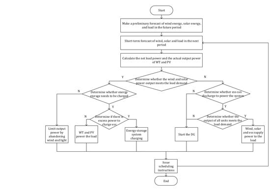
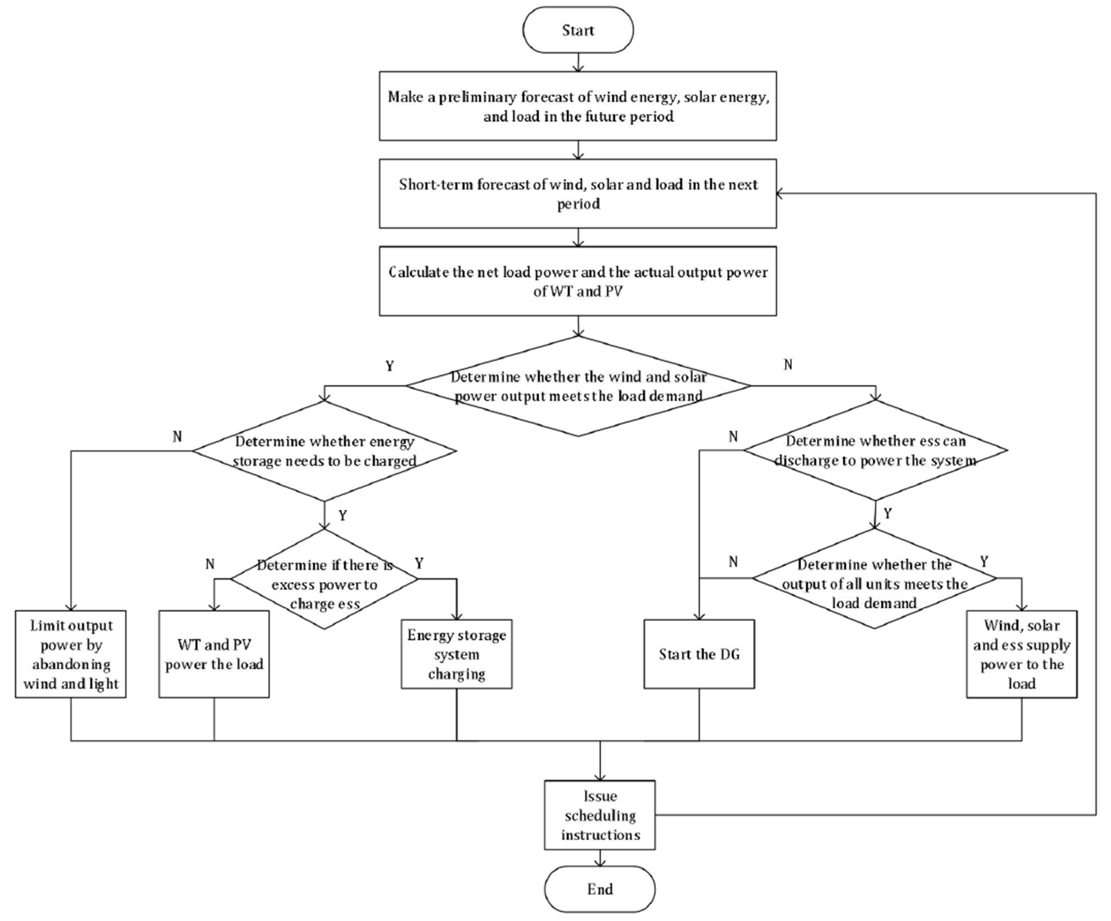
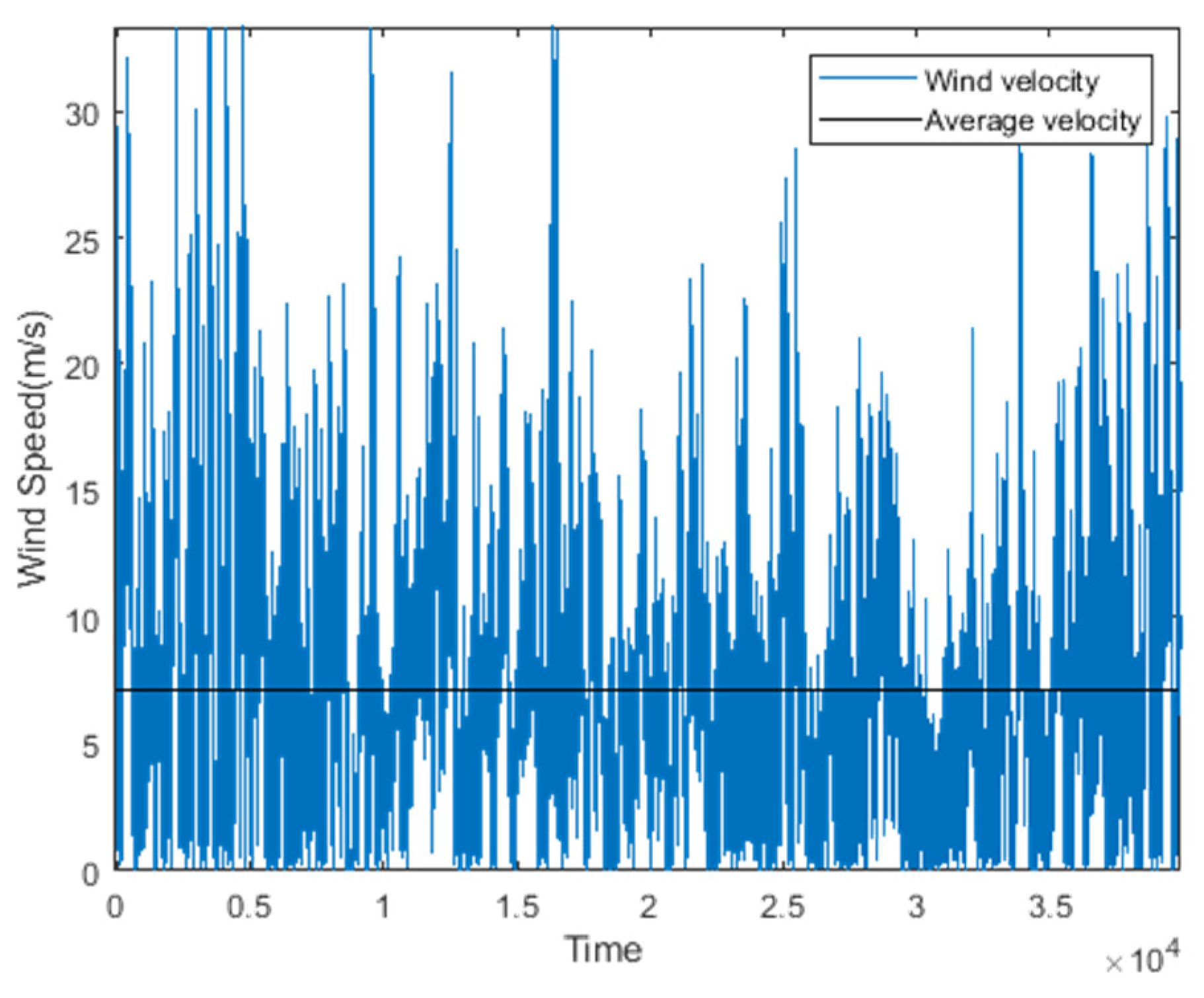
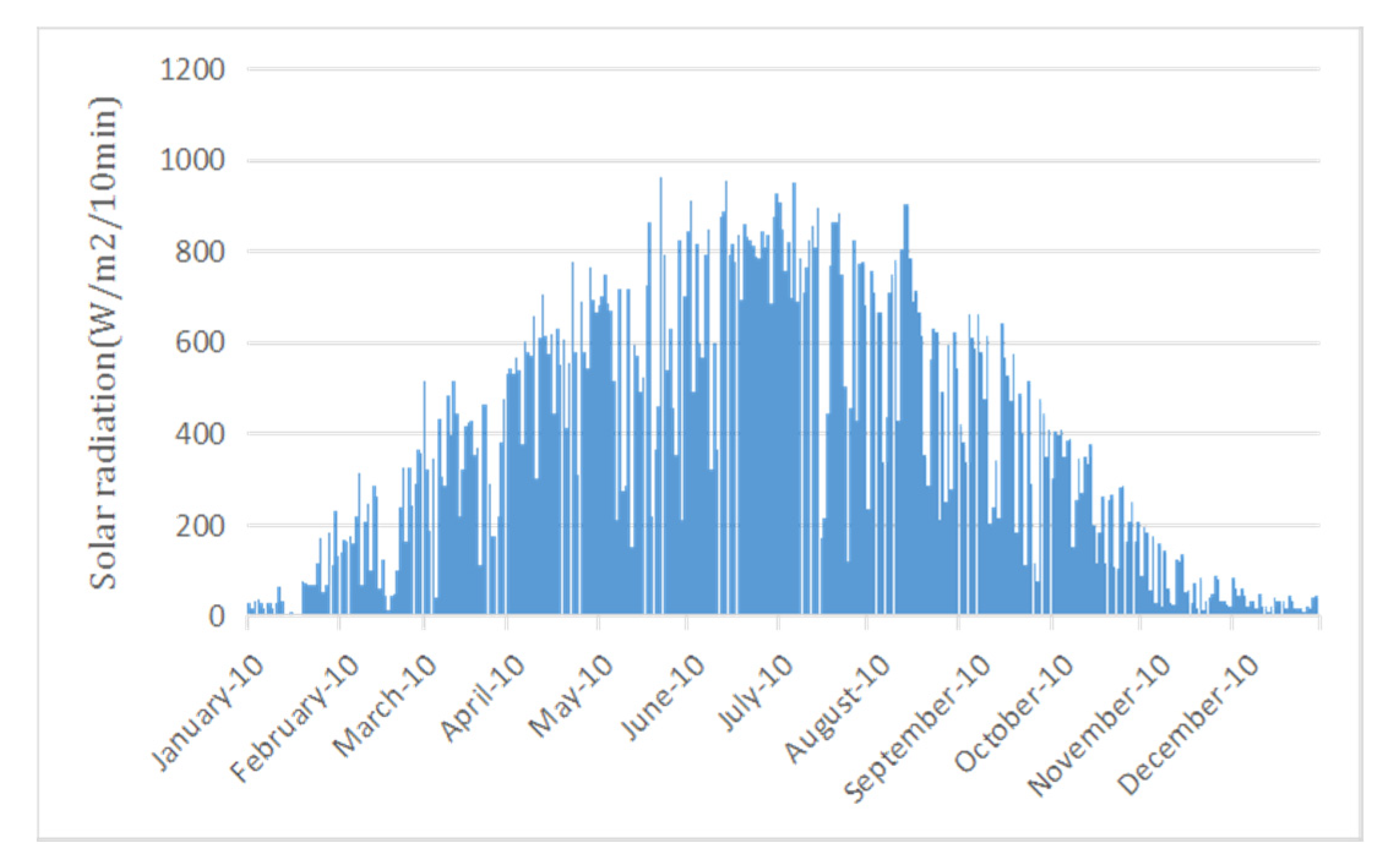
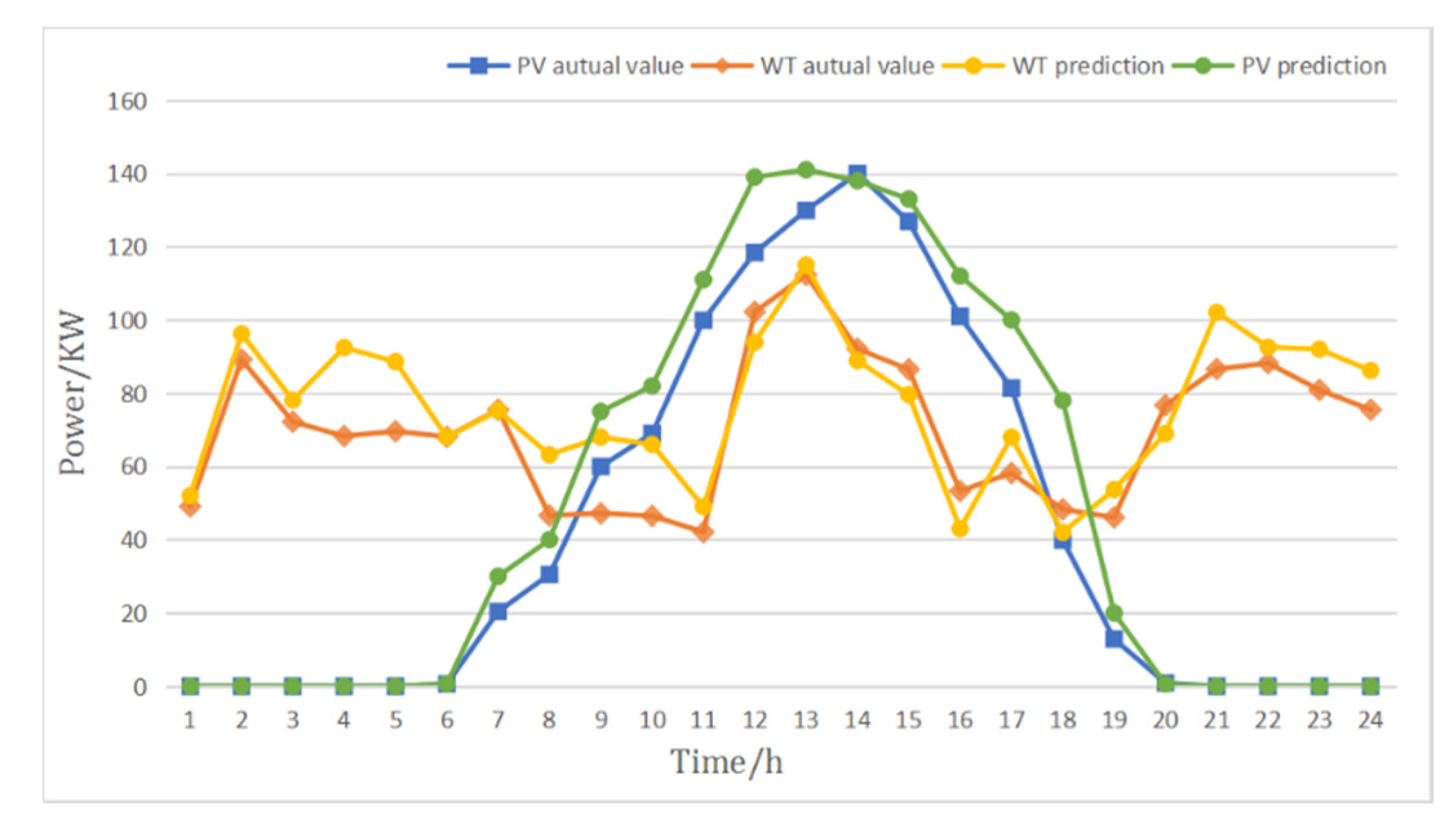
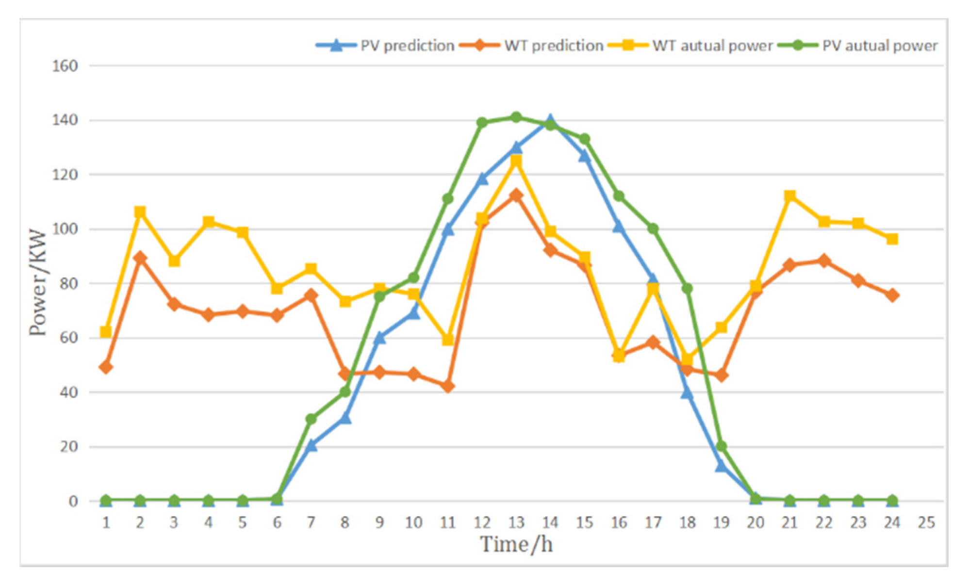
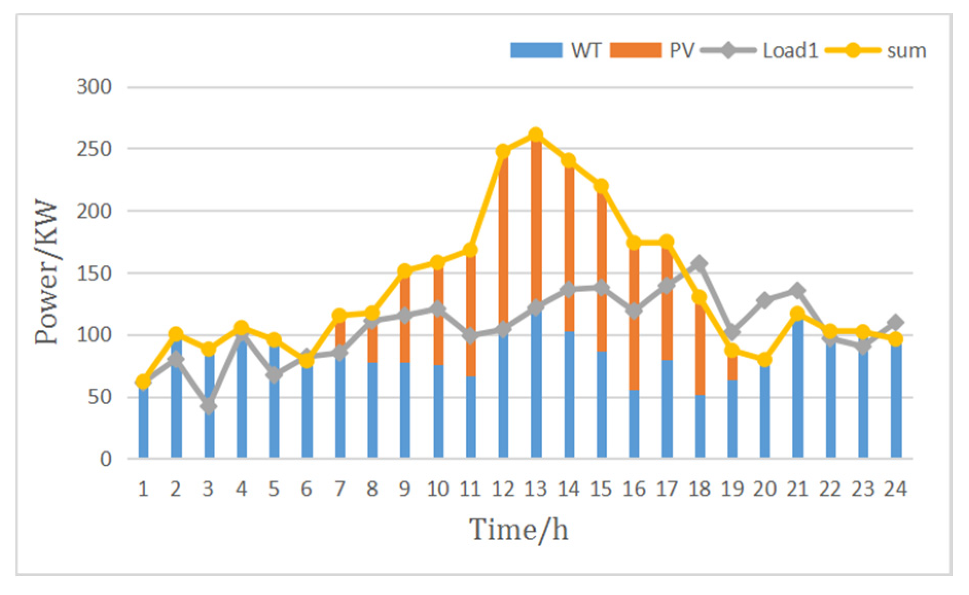
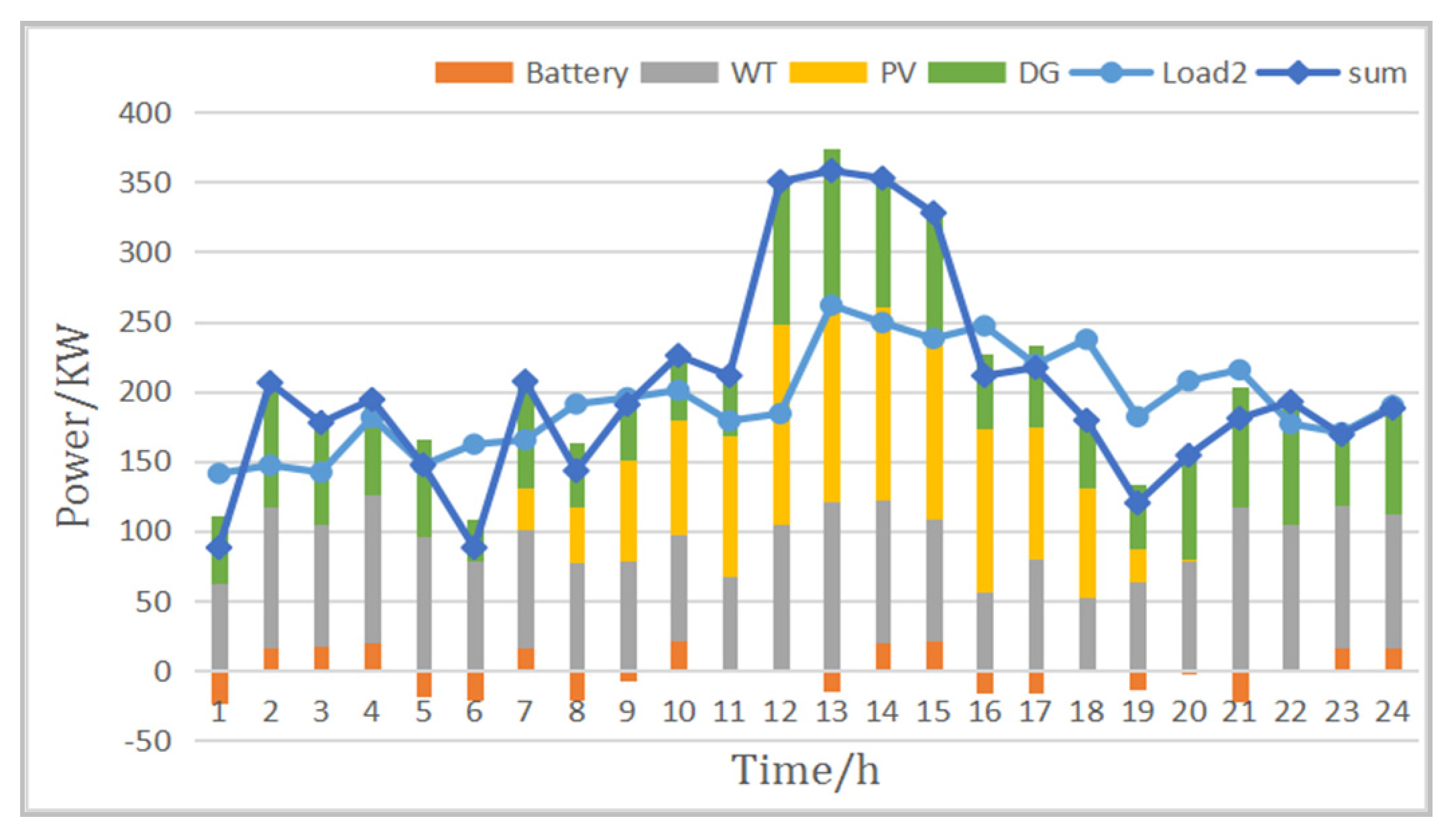
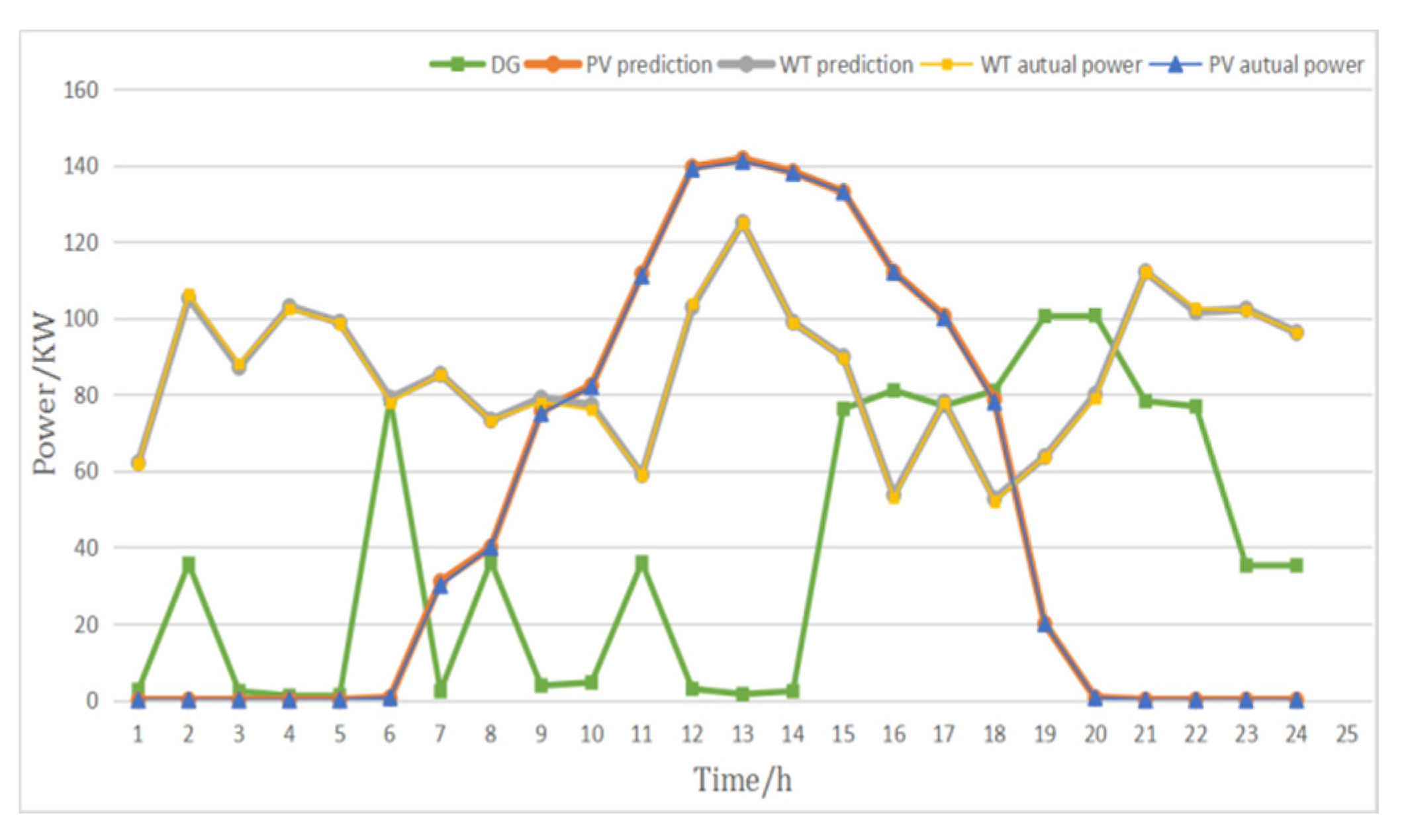
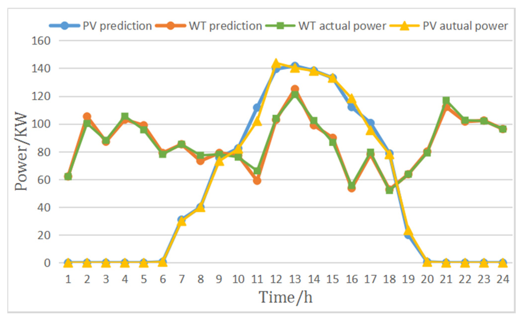
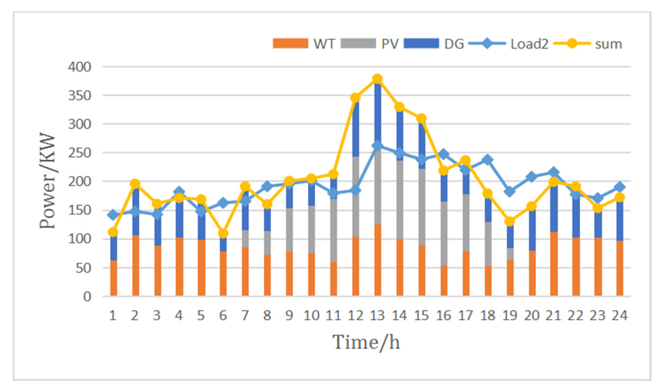
In order to solve the problem of optimal operation and scheduling of islanded microgrid, it is usually more effective to use the energy optimization management method with multi-period coordination. The flow chart in Figure 2 demonstrates the scheduling strategy proposed in this paper. Since the islanded microgrid system can only use the power output power of the WT and PV power generation system, it is necessary to predict the wind, solar and load demand in the future in advance. Due to the volatility of wind and solar energy, further short-term forecasting of wind and solar energy is needed to ensure the accuracy of the forecast. After obtaining the forecast data of wind energy, solar energy and load, it is divided into 6 different scenarios.

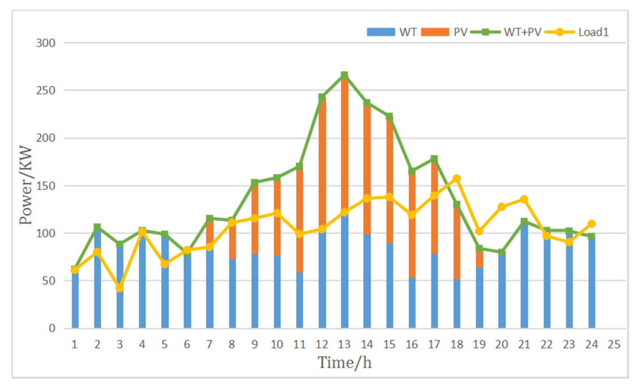
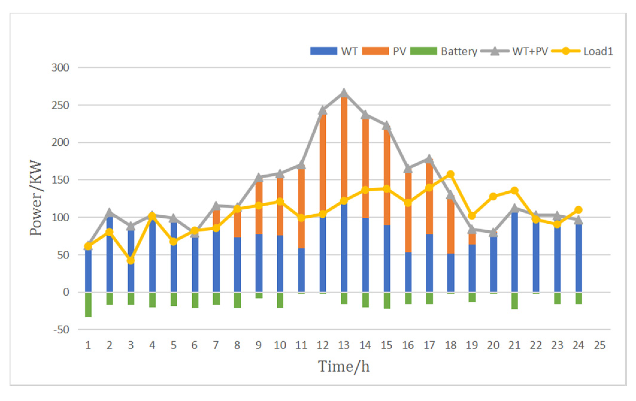
Scenario 1: When the electrical energy generated by the WT and PV can meet the demand of the load, it should then be determined whether the ess needs to be charged. When the state of charge is sufficient and charging is not required, the power output of the WT and PV is limited by abandoning the wind and the light.

Scenario 2: When the state of charge of the ess is insufficient and charging is required, it is further determined whether there is excess electrical energy for energy storage. If there is excess electrical energy, the ess is charged after meeting the load demand.

Scenario 3: If there is no excess power, the WT and PV output only need to meet the power supply of the load.

Scenario 4: If there is no excess electrical energy, the WT and PV output can only meet the load power supply. When the power generated by the WT and PV is insufficient to meet the load demand, it is necessary to determine whether the ess can be discharged to supplement the power. If ess does not have enough power to power the load, then need to start diesel generators to power the system load.

Scenario 5: If ess can supply power, it needs to further determine whether the total output of WT/PV and ess meet the load demand. If the output meets the need, then the wind, solar and energy storage system is used to supply power to the load.

Scenario 6: If the output cannot meet the load, it also needs to start diesel generators to supply power to the system load.

The flow chart in Figure 2 is the scheduling strategy proposed in this section.

Optimal Sizing of Microgrid Using GWO

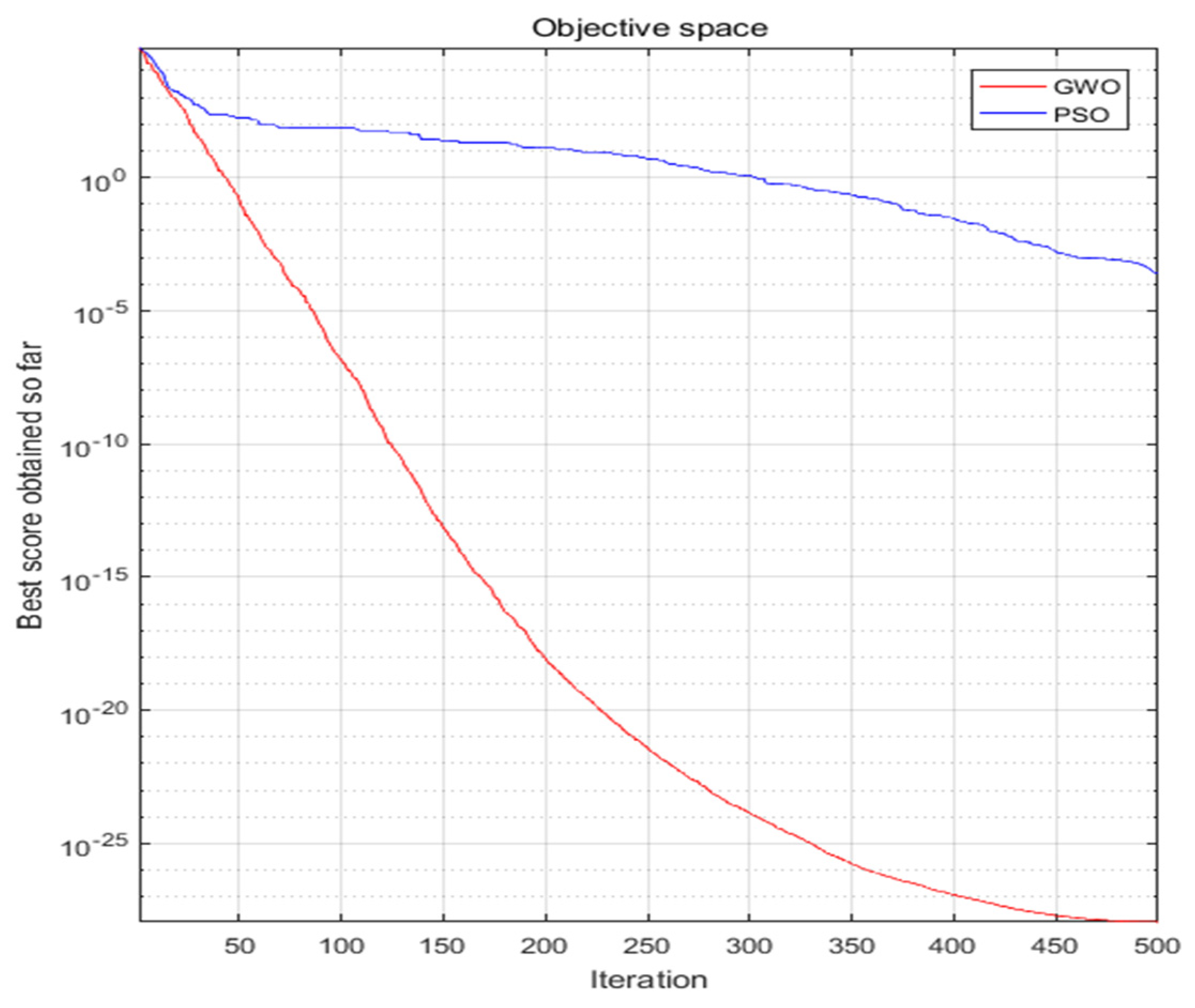
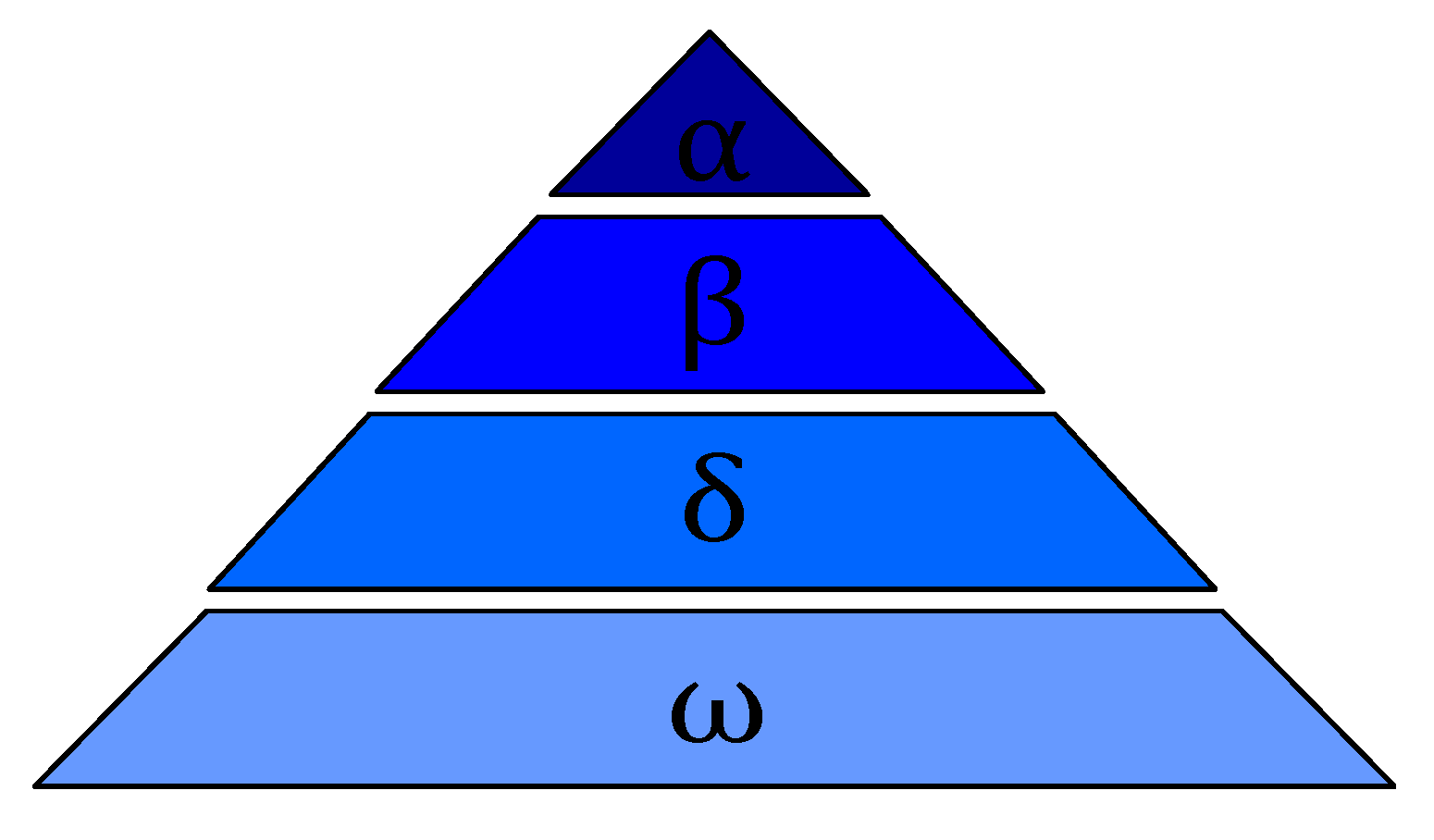
Grey Wolf Optimization (GWO) is a group intelligence optimization algorithm proposed by Griffith University scholar Mirjalili and others in Australia in 2014. The algorithm is an optimized search method developed by the grey wolf predator activity. It has the characteristics of strong convergence performance, few parameters, and easy implementation [29]. Grey wolves belong to canines that live in groups and are at the top of the food chain. The grey wolf strictly observes a hierarchy of social dominance. As shown in Figure 3.

The GWO optimization process includes five steps. The specific steps are as follows.

(a) Social Hierarchy

First, wolf pack and set the number are initialized, then the fitness value of each individual in the wolf pack are calculated. Mark the grey wolves with the top three fitness values as α, β, δ, and the remaining wolves as ω. That is to say, the social rank in the grey wolf group is ranked from high to low in order of α, β, δ, and ω. The three optimal solutions (α, β, δ) in each iteration guide the optimization process of GWO.

(b) Encircling Prey

The grey wolf will gradually approach the prey and surround it when it searches for the prey. The functional expression for this behavior is as follows [29]:

$$\begin{array}{c}D=C\circ X_p(t)-X(t)\\ X(t+1)= X_p(t)-A\circ D\\ A=2a\circ r_1-a\\ C=2r_2\end{array}$$

(18)

where t is the current number of iterations, A and C are the synergy coefficients; vector X_p represents the position vector of the prey; X(t) represents the current grey wolf’s position vector; a linearly decreases from 2 to 0 during the entire iteration process; r₁ and r₂ are the random vector in [0, 1].

(c) Hunting

The grey wolf has the ability to identify the position of the potential prey (optimal solution). However, the solution space characteristics of many problems are unknown, and the grey wolf cannot determine the precise position of the prey.

In order to get the best optimization plan, it is assumed that α, β, δ have the ability to identify the possible location of prey to simulate the behavior of grey wolf. Therefore, keep the best three grey wolves (α, β, δ) in the current population during iterating, then update their positions according to the positions of other search agents (including ω). The mathematical model of this behavior can be expressed as follows [29]:

$$\begin{array}{c}{D}_{\alpha }=C_1\circ X_{\alpha }-X, D_{\beta }=C_2\circ X_{\beta }-X, D_{\delta }=C_3\circ X_{\delta }-X\\ X_1=X_{\alpha }-A_1\circ D_{\alpha }, X_2=X_{\beta }-A_2\circ D_{\beta }, X_3=X_{\delta }-A_3\circ D_{\delta }\\ X(t+1)=\frac{X_1+X_2+X_3}{3}\end{array}$$

(19)

where X_α, X_β, X_δ represent the position vector of α, β, δ in the current population; X represent the position vector of the grey wolf; D_α, D_β, D_δ represent the distance between the current search agent and the best three wolves; when the |A>1|, the gray wolf searches for prey in different areas as much as possible. When |A<1|, grey wolves focused on searching for prey within a certain area.

(d) Attacking Prey

In the process of constructing the attacking prey model, according to (b), the decrease of a value will cause the value of to fluctuate accordingly. In other words, is a random vector in the interval [−a, a]. When is in [−1, 1] interval, the search agent’s position can be anywhere between the current grey wolf and its prey at the next moment.

(e) Search for Prey

Grey wolves mainly rely on the information of α, β, and δ to find their prey. In the process of searching for prey, keeping the search agent away from the prey can make the grey wolf perform a global search. In formula (b), the C vector composed of random values in the interval range [0, 2]. The random search behavior of grey wolves can make the optimization results more accurate and avoid falling into local optimum. C is a random value during the iteration process. This coefficient is helpful for the algorithm to jump out of the local area, especially the algorithm is particularly important in the later stage of the iteration.

After the microgrid obtains real-time information on the system status, it begins to execute the GWO. First, it sets the number of wolves and initializes the wolves, and then calculates the fitness value of each wolf. The top three are recorded as α, β, δ each wolf updates its position by calculating the distance from α, β, δ and finally outputs the global optimal solution, according to whether the maximum number of iterations is reached. Some of the previous optimization algorithms are prone to fall into the shortcomings of local optimization, slow convergence, and optimization of the microgrid. The flow chart in Figure 4 is the microgrid dispatching process combined with the GWO.

6. Case Study and Simulation Results

Sanya is located south of the Tropic of Cancer and has a tropical monsoon climate characterized by high temperature and rain. All relevant data are obtained from the official website of the local meteorological bureau. The annual average temperature is 26.7 °C. The highest temperature month is June with an average of 29.7 °C. The lowest temperature month is January with an average of 22.4 °C. The sunshine time of the year is 2534 h. The average annual precipitation is 1347.5 mm. Known as the “natural greenhouse”.

6.1. Case Study

Figure 5 and Figure 6 show the hourly wind speed and solar radiation data. However, due to the instability of wind energy and the tendency of wind density to change, this brings certain challenges to research. In order to ensure that the energy generated by the system can be balanced with the load demand. In this paper, we use the Artificial Neural Networks(ANN) to forecast the wind power. Figure 7 shows the regression graph obtained using ANN training test data including wind speed and solar radiation. We see that 0.96316 in the 40th iteration, which demonstrates a high correlation between the results obtained after training and the target. In addition, most of the results generated by the training data are related to the best fit line.

6.2. Description of the System

The basic parameters of the WT, PV and diesel generator equipment in the microgrid system are shown in

Table 1. Basic parameters of WT, PV and DG.

Components	Installed Capacity (kW)	UP Cost ($/kW)	UP Operation and Maintenance Cost ($/kW)	Power Generation Cost ($/kW)
				a	b	c
WT	100	112	0.0042		0
PV	150	24	0.0013		0
DG	100	12	0.0245	0	0.24	0.0035

. The rated capacity of the configured single battery is 50% of the total installed capacity of PV and WT [30]. Other parameters of the battery are shown in

Table 2. Energy Storage System Parameters.

Parameter	Value	Parameter	Value
type	ess	Max charge & discharge power/kW	50
Capacity/kWh	50 × 5	Initial capacity/kW	50
Max allowable state of charge	95%	Charging efficiency	15
Min allowable state of charge	15%	Discharging efficiency	95%

The maximum discharge depth is 80%, and the operation and maintenance cost coefficient is 0.009 $/kWh [32].

. In this paper, there are three main types of air pollutants emitted during the operation of diesel generators: CO₂, NOx and SO₂ [31]. The corresponding emissions and environmental treatment costs are shown in

Table 3. Corresponding Environmental Value of Pollutants.

Pollution	CO2	NOx	SO2
Emissions (g/kWh)	649.05	9.33	0.46
Value ($/KG)	0.0288	8.9747	2.1328

.

6.3. Simulation Results

In this paper, MATLAB R2019a is used for simulation and comparison of results. The response comparison of the microgrid system under different algorithms is shown in Figure 8 and Figure 9. It can be seen from Figure 8 that using the GWO algorithm to solve the optimization scheduling problem of the microgrid is faster than the standard PSO algorithm, and it is easier to obtain the optimization results. Figure 9 shows the comparison of the parameter space of the two algorithms. It can be seen from Figure 8 and Figure 9 that GWO has a faster convergence speed, and it is easier to obtain optimization results, and there is no local optimal situation in the figure.

Table 4. Simulation Results of Test System Error.

	GWO		PSO
	Ave	Std	Ave	Std
S1	−10.086523	12.233906	0.000136	0.000202
S2	2.517264	0.029014	0.042144	0.045421
S3	2.943147	79.14958	70.12562	22.11924
S4	8.249561	1.315088	1.086481	0.317039
S5	0.816579	0.000126	0.000102	17.50737
S6	0.002213	0.100286	0.122854	0.044957

shows the standard and average solutions of GWO are better than PSO, and compared with the PSO algorithm, GWO does not show the worst solution with a large deviation from the optimal solution. Its standard deviation is also much smaller than the standard deviation of PSO. As seen in Figure 8, GWO convergence speed is faster than PSO, it is not easy to fall into the local optimal, obtaining the global optimal solution is faster, the result is better, and the efficiency of the algorithm is higher.

The simulation results of the algorithm are better than PSO, which verifies that this paper is effective in optimizing the scheduling of microgrid system with GWO, and has superiority in convergence speed and optimization results compared with PSO.

6.4. Analysis of Optimal Dispatching Results of Microgrid

In Section 5, the optimized scheduling strategy proposed in this paper is presented, and the optimized scheduling strategy of microgrid with multiple time periods is used to divide the optimized scheduling strategy into 6 scenarios. In this part of the study, the output of each group of equipment in these 6 scenarios will be demonstrated, and the costs and pollutant emissions in each scenario will be compared.

Scenario 1 will determine whether the battery energy storage system needs to be charged when the power generated by WT and PV can meet the load demand. When the battery is in a sufficient state of charge and does not need to be charged, the power output of WT and PV is limited by abandoning wind and light. The predicted and the actual wind and solar values at each moment in Scenario 1 are shown in Figure 10. Under the condition of the Load1 which indicates the normal load size, the best output under constraints in Scenario 1 is shown in Figure 11. It can be seen from the figures that when the wind and solar resources are sufficient, while the ess system does not need to be charged, and the load demand is not large, the output of WT and PV can meet the load demand, so it does not need to run the diesel generator.

In Scenario 2, it is carried out under the same normal load demand as in Scenario 1 while the battery has insufficient power and needs to be charged. It is necessary to further determine whether the wind and solar power generation has excess power after supplying the load to charge the battery, Scenario 2 shows that there is excess electric energy to charge the ess, so the ess is charged after the load demand is met. The predicted wind and solar values are the same as shown in Figure 10. The best output of WT and PV under constraints in Scenario 2 is shown in Figure 12.

It can be found in Figure 12 that part of the wind and solar power generation capacity can charge the ess when the load demand is not large, which can consume more clean energy and the ess plays a role in the coordinated control of the system.

Scenario 3 shows that when the load demand is not large and the energy storage system needs to be charged, but if there is no excess electric energy to charge the energy storage system, the output of WT and PV only needs to meet the power supply demand of the load. The predicted and the actual wind and solar values at each moment in Scenario 3 are shown in Figure 13. Under the condition the best output under constraints is shown in Figure 14.

Different from the first three scenarios, scenarios 4–6 are carried out when the load demand is large. In Scenario 4, the wind and solar power generation is insufficient to meet the load demand, so it is necessary to determine whether the ess can discharge to give the load power supply, when ess does not have enough power to power the load, then need to start the diesel generator to power the load. Figure 15 shows the predicted and the actual wind, solar and DG power at each moment in Scenario 4. Figure 16 shows the best output under constraints.

In Scenario 5, the load demand is large but ess has energy storage to supply power to the load and WT, PV and ess can meet the load demand. In this scenario, the predicted output value and actual output power of the scenery are shown in Figure 17, the best output under the conditions is shown in Figure 18.

Scenario 6 is the last scenario of the study, and it is carried out under the condition of large load demand like Scenarios 4, 5, but at this time, ess has no electrical energy to power the load, so it is necessary to start the diesel generator to meet the load demand. The predicted wind and solar values are the same as shown in Figure 15. The best output of WT and PV under constraints in Scenario 6 is shown in Figure 19.

Under Load2, the wind power, PV power generation and energy storage systems can no longer meet the system load demand. The diesel generator in the system must be started, in order to make up for the power shortage of the system. The operating conditions are closely related, that is, there is a minimum output power and an optimal output power. In addition, the charge and discharge state of the ess under Load 2 is switched more frequently. From Figure 15, it can be seen that the diesel generator reaches full-running state from 19 to 20 o’clock. Compared with Load1, the consumption of wind power and photovoltaic power generation is higher under Load2 conditions, so the total cost is higher than the total cost under Load1. However, as Load2 requires more energy, making wind power and photovoltaic power generation so the energy utilization rate is also higher.

The comparison of the optimized scheduling results in 6 different scenarios is shown in Figure 20 and

Table 5. The comparison of the system optimal scheduling results under 6 different scenarios.

Dispatching Results	Scenario 1	Scenario 2	Scenario 3	Scenario 4	Scenario 5	Scenario 6
Total power (kWh)	122,998	123,072	123,524	124,207	124,524	124,632
Total emissions (kg)	61,755	62,157	64,625	71,070	70,251	81,439
Total cost ($)	50,441	50,577	63,077	64,961	64,736	65,046
wind power (kWh)	10,941	10,941	10,941	36,327	36,327	36,327
PV power (kWh)	1330	1330	1330	6549	6549	6549
wind power utilization (%)	70.73	70.12	60.66	86.40	82.33	87.15
PV power utilization (%)	78.63	70.26	74.68	98.76	99.16	98.76
Renewable energy utilizaition rate (%)	74.68	70.19	67.67	92.58	90.75	92.96
Renewable energy output fuluctuations	26,891.16	28,121.92	4225.39	9859.25	15,568.06	10,322.18
Residual power generation capacity of WT and PV (kWh)	3486.65	3664.71	4640.95	5021.68	6473.99	4749.23

. As can be seen in Figure 20, when the load demand is larger, the utilization rate of clean energy is also higher, but from Table 5 it can be seen that the larger the load demand, the higher the total cost of the microgrid system, and the more environmental pollution emissions caused by starting the diesel generator. Among these 6 different scenarios, Scenarios 1, 3, and 5 are more ideal scenarios. In our daily life, diesel generators are often used to supply power to the load, so the emission of polluting gases is inevitable. The environmental cost of the system will increase accordingly. The comparison of optimized scheduling results in 6 different scenarios is shown in Figure 20.

Table 5 shows the comparison of the system optimal scheduling results under 6 different scenarios. As can be seen from the table, when the load demand is large, the system’s total power generation is the largest, but the total cost is also the highest, because the diesel generator is started. Therefore, the emission of polluting gas is also the most, so the cost of environmental governance will increase. However, on the other hand, due to the increase in electrical energy required, the utilization rate of renewable energy has reached a maximum of 92.96%, reducing wind and light, and the battery energy storage system has also played a role in cutting the valley and filling the peak effect.

7. Conclusions

This paper presents an optimal sizing of an islanded microgrid, optimized by dynamic optimization with GWO. The considered microgrid is a small autonomous system that integrates a variety of clean energy distributed power generation systems, energy storage systems, backup power sources, and electrical loads. Due to the complexity of optimal scheduling, a multi-objective optimal scheduling method combining GWO and dynamic optimal scheduling is proposed. Moreover, a comparison between the optimization capabilities of GWO and PSO on the one hand, and the system is divided into six different scenarios for comparison on the other, in order to understand the best output that achieves the lowest total cost of microgrid system operation and the highest clean energy utilization rate. Meteorological data is used, which is measured by the local meteorological bureau, in addition to artificial neural networks used to predict wind and solar energy in the future for a residential area in Sanya, China. The results show that the advantage of combining the GWO solution in optimizing multi-objective problems lies in that it reduces the calculation time and obtains the best function value compared with the PSO method alone. Furthermore, the findings of the study illustrate the economic and environmental feasibility of starting diesel generators under heavy load demand. Using ess as storage can better play the role of peak and valley filling, thereby reducing the total cost of the system. By considering diesel generators as part of the hybrid power system, the utilization of renewable energy can be improved. However, the use of diesel generators will produce polluting gas emissions. To solve this problem, multi-objective optimization based on GWO is applied. The optimal scale of the hybrid system including PV/wind/ess/diesel generators is a total cost of $64961 and 71070 kg.

In the future, the multi-objective optimization problem of microgrid can be further studied. Secondly, this paper studies the dynamic optimal dispatching of islanded microgrid. The economics of grid-connected microgrid and the utilization rate of clean energy generation must be studied in depth. Finally, because we use GWO for optimization, we can make the method more competitive by adjusting the scheduling strategy.

References

1. Lasseter, R.H.; Piagi, P. Microgrid: A conceptual solution. In Proceedings of the IEEE Power Electronics Specialists Conference, Aachen, Germany, 20–25 June 2004; pp. 4285–4291. [Google Scholar]
2. Hamad, A.A.; Azzouz, M.A.; El-Saadany, E.F. Multiagent supervisory control for power management in DC microgrids. IEEE Trans. Smart Grid. 2016, 7, 1057–1068. [Google Scholar] [CrossRef]
3. Dunham, H.; Cutler, D.; Mishra, S.; Li, X. Cost-optimal evaluation of centralized and distributed microgrid topologies considering voltage constraints. Energy Sustain. Dev. 2020, 56, 88–97. [Google Scholar] [CrossRef]
4. Dai, R.; Liao, H.; Shi, Y.Z.; Liao, Y.; Xia, H.B.; Chen, M.Y. Economic dispatch method of microgrid considering demand response under time-of-use electricity price. J. Chongqing Univ. 2019, 122, 36–52. [Google Scholar]
5. Mileta, Ž.; Goran, D. Fuzzy expert system for management of smart hybrid energy microgrid. J. Renew. Sustain. Energy 2019, 11, 034101. [Google Scholar]
6. Dey, B.; Bhattacharyya, B.; Sharma, S. Optimal Sizing of Distributed Energy Resources in a Microgrid System with Highly Penetrated Renewables. Iran. J. Sci. Technol. Trans. Electr. Eng. 2018, 43, 527–540. [Google Scholar] [CrossRef]
7. Yuan, D.; Lu, Z.; Zhang, J.; Li, X. A hybrid prediction-based microgrid energy management strategy considering demand-side response and data interruption. Electr. Power Energy Syst. 2019, 260, 139–153. [Google Scholar] [CrossRef]
8. Li, X.; Tang, R.; Lai, J. A Knowledge based Multi-objective Optimization Strategy for Microgrid Environmental or Economic Scheduling problems. Energy Procedia 2019, 182, 2942–2947. [Google Scholar] [CrossRef]
9. Gildenhuys, T.; Zhang, L.; Ye, X.; Xia, X. Optimization of the Operational Cost and Environmental Impact of a Multi-Microgrid System. Energy Procedia 2019, 182, 3827–3832. [Google Scholar] [CrossRef]
10. Kumar, D.; Verma, Y.P.; Khanna, R. Demand response-based dynamic dispatch of microgrid system in hybrid electricity market. Int. J. Energy Sect. Manag. 2019, 13, 318–340. [Google Scholar] [CrossRef]
11. Ismail, M.S.; Moghavvemi, M.; Mahlia, T.M.I. Genetic algorithm based optimization on modeling and design of hybrid renewable energy systems. Energy Convers. Manag. 2014, 85, 120–130. [Google Scholar] [CrossRef]
12. Ko, M.J.; Kim, Y.S.; Chung, M.H.; Jeon, H.C. Multi-Objective Optimization Design for a Hybrid Energy System Using the Genetic Algorithm. Energies 2015, 8, 2924–2949. [Google Scholar] [CrossRef] [Green Version]
13. García-Triviño, P.; Llorens-Iborra, F.; García-Vázquez, C.A.; Gil Mena, A.J.; Fernández-Ramírez, L.M.; Jurado, F. Long-term optimization based on PSO of a grid-connected renewable energy/battery/hydrogen hybrid system. Int. J. Hydrog. Energy 2014, 39, 10805–10816. [Google Scholar] [CrossRef]
14. Azim, H.; Davide, A.G.; Farshid, K.; Fabio, B. Renewable Energies Generation and Carbon Dioxide Emission Forecasting in Microgrids and National Grids using GRNN-GWO Methodology. Energy Procedia 2019, 159, 154–159. [Google Scholar]
15. Naderi, E.; Azizivahed, A.; Narimani, H.; Fathi, M.; Narimani, M.R. A comprehensive study of practical economic dispatch problems by a new hybrid evolutionary algorithm. Appl. Soft Comput. 2017, 61, 1186–1206. [Google Scholar] [CrossRef]
16. Nuaekaew, K.; Artrit, P.; Pholdee, N.; Bureerat, S. Optimal reactive power dispatch problem using a two-archive multi-objective grey wolf optimizer. Expert Syst. Appl. 2017, 87, 79–89. [Google Scholar] [CrossRef]
17. Dong, Y.; Cai, Z. Research on control strategy of isolated island microgrid based on synchronous inverter technology. In Proceedings of the 16th Shenyang Scientific Academic Conference, Shenyang, China, 9–30 October 2019. [Google Scholar]
18. Fan, S.; Xiong, H.W. Dynamic reactive power optimization model of power grid considering VSC and DFIG. Power Syst. Prot. Control. 2019, 36, 28–36. [Google Scholar]
19. Wu, C.; Lin, S.; Xia, C.J.; Guan, H. Distributed optimal dispatch of microgrid group based on model predictive control. Power Syst. Technol. 2019, 111, 30–39. [Google Scholar]
20. Wu, S.; Yu, J.; Tian, Z.; Zhang, L.Z.; Yang, W.; Li, Y.; Peng, L.; Wu, W. Unified power flow algorithm for AC/DC hybrid power grid based on extended node method. Power Syst. Prot. Control. 2018, 70, 22–30. [Google Scholar]
21. Fu, Y.; Sang, Y. The EU’s REserviceS project and its enlightenment for China’s wind power and photovoltaic participation in grid frequency regulation. Power Syst. Technol. 2019, 10, 1–6. [Google Scholar]
22. Shan, C.; Gao, C.S.; Long, L.Z.; Tian, L.H. Dynamic dispatch optimization of microgrid based on a QS-PSO algorithm. J. Renew. Sustain. Energy 2017, 9, 045505. [Google Scholar]
23. Abdelshafy, A.M.; Hassan, H.; Jurasz, J. Optimal design of a grid-connected desalination plant powered by renewable energy resources using a hybrid PSO–GWO approach. Energy Convers. Manag. 2018, 173, 331–347. [Google Scholar] [CrossRef]
24. Diaf, S.; Diaf, D.; Belhamel, M.; Haddadi, M.; Louche, A. A methodology for optimal sizing of autonomous hybrid PV/wind system. Energy Policy 2007, 35, 5708–5718. [Google Scholar] [CrossRef] [Green Version]
25. Azad, H.B.; Mekhilef, S.; Ganapathy, V.G.; Modiri-Delshad, M.; Mirtaheri, A. Optimization of micro-grid system using MOPSO. Renew. Energy 2014, 71, 295–306. [Google Scholar]
26. Yin, C.; Wu, H.; Locment, F.; Sechilariu, M. Energy management of DC microgrid based on photovoltaic combined with diesel generator and supercapacitor. Energy Convers. Manag. 2017, 132, 14–27. [Google Scholar] [CrossRef]
27. Bilal, B.O.; Nourou, D.; Sambou, V.; Ndiaye, P.A.; Ndongo, M. Multi-objective optimization of hybrid PV/wind/diesel/battery systems for decentralized application by minimizing the levelized cost of energy and the CO2 emissions. Int. J. Phys. Sci. 2015, 10, 192–203. [Google Scholar]
28. Bukar, A.L.; Tan, C.; Lau, K.Y. Optimal sizing of an autonomous photovoltaic/wind/battery/diesel generator microgrid using grasshopper optimization algorithm. Sol. Energy 2019, 188, 685–696. [Google Scholar] [CrossRef]
29. Fescioglu-Unver, N.; Barlas, A.; Yilmaz, D.; Demli, U.O.; Bulgan, A.C.; Karaoglu, E.C.; Atasoy, T.; Ercin, O. Resource management optimization for a smart microgrid. J. Renew. Sustain. Energy 2019, 11, 065501. [Google Scholar] [CrossRef]
30. Zhang, X.; Wang, X. A review of grey wolf optimization algorithm. Comput. Sci. 2019, 46, 30–38. [Google Scholar]
31. Zhao, B.; Zhang, X.; Chen, J.; Wang, C.; Guo, L. Operation Optimization of Standalone Microgrids Considering Lifetime Characteristics of Battery Energy Storage System. IEEE Trans. Sustain. Energy 2013, 4, 934–943. [Google Scholar] [CrossRef]
32. Das, A.; Ni, Z. A Computationally Efficient Optimization Approach for Battery Systems in Islanded Microgrid. IEEE Trans. Smart Grid 2017, 9, 6489–6499. [Google Scholar] [CrossRef]
Figure 1. Basic structure diagram of islanded microgrid.
Symmetry 12 01366 g001
Figure 2. The scheduling strategy of the microgrid.
Symmetry 12 01366 g002
Figure 3. Grey wolf social dominance hierarchical relationship.
Symmetry 12 01366 g003
Figure 4. Flowchart for microgrid dispatching process combined with the GWO.
Symmetry 12 01366 g004
Figure 5. Annual wind speed of the studied location.
Symmetry 12 01366 g005
Figure 6. Annual solar irradiance of the location.
Symmetry 12 01366 g006
Figure 7. Regression of wind power ANN.
Symmetry 12 01366 g007
Figure 8. A comparison between algorithms.
Symmetry 12 01366 g008
Figure 9. The parameter space of the two algorithms.
Symmetry 12 01366 g009
Figure 10. The predicted and actual value of WT and PV in Scenario 1.
Symmetry 12 01366 g010
Figure 11. The best output under constraints in Scenario 1.
Symmetry 12 01366 g011
Figure 12. The best output under constraints in Scenario 2.
Symmetry 12 01366 g012
Figure 13. The predicted and actual value of WT and PV in Scenario 3.
Symmetry 12 01366 g013
Figure 14. The best output under constraints in Scenario 3.
Symmetry 12 01366 g014
Figure 15. The predicted and actual value of WT, PV and DG in Scenario 4.
Symmetry 12 01366 g015
Figure 16. The best output under constraints in Scenario 4.
Symmetry 12 01366 g016
Figure 17. The predicted and actual value of WT and PV in Scenario 5.
Symmetry 12 01366 g017
Figure 18. The best output under constraints in Scenario 5.
Symmetry 12 01366 g018
Figure 19. The best output under constraints in Scenario 6.
Symmetry 12 01366 g019
Figure 20. The comparison of optimized scheduling results in 6 different scenarios.
Symmetry 12 01366 g020