Article

Bivariate Power-Skew-Elliptical Distribution

by
Guillermo Martínez-Flórez
1,2,†,
Roger Tovar-Falón
1,† and
Héctor W. Gómez
3,*,†
1
Departamento de Matemáticas y Estadística, Facultad de Ciencias Básicas, Universidad de Córdoba, Montería 230027, Colombia
2
Programa de Pós-Graduação em Modelagem e Métodos Quantitativos, Universidade Federal de Ceará, Fortaleza 60020-181, Brazil
3
Departamento de Matemáticas, Facultad de Ciencias Básicas, Universidad de Antofagasta, Antofagasta 1240000, Chile
*
Author to whom correspondence should be addressed.
These authors contributed equally to this work.
Symmetry 2020, 12(8), 1327; https://doi.org/10.3390/sym12081327
Submission received: 4 July 2020 / Revised: 3 August 2020 / Accepted: 5 August 2020 / Published: 9 August 2020

Abstract

:
In this article, we introduce a power-skew-elliptical (PSE) distribution in the bivariate setting. The new bivariate model arises in the context of conditionally specified distributions. The proposed bivariate model is an absolutely continuous distribution whose marginals are univariate PSE distributions. The special case of the bivariate power-skew-normal (BPSN) distribution is studied in details. General properties of the BPSN distribution are derived and the estimation of the unknown parameters by maximum pseudo-likelihood is discussed. Further, a sandwich type matrix, which is a consistent estimator for the asymptotic covariance matrix of the maximum likelihood (ML) estimator is determined. Two applications for real data of the proposed bivariate distribution is provided for illustrative purposes.

1. Introduction

Family of distributions that unify the main characteristics of other families are not very common in distributions theory. In this sense, an asymmetric family widely used in many situations and different areas of knowledge is the skew-normal (SN) distribution of [1], that is characterized because it has a wide range of asymmetry. Another well-known family in this same area is the fractional order statistical distribution, also known as exponentiated distribution or power-normal distribution introduced by [2], which is characterized by having a wide range of kurtosis. The unification of these two families was studied by [3] and was called power-skew-normal distribution. The resulting family contains, such as special cases the normal, skew-normal and power-normal distributions, and the ranges of asymmetry and kurtosis are greater than any of these three families of distributions. This type of unification of distribution families is important in the literature of distribution theory because it introduces great flexibility to the resulting models.
This model was extended to the case of elliptical distributions and was considered the case of the Birnbaum-Saunders (BS) family by [4], resulting in a large unification of useful distributions for example, to model the lifetime in survival analysis or applications in reliability theory. The model is called Birnbaum-Saunders power skew elliptical (BSPSE), and it contains as special cases as a large number of extensions of the lifetime Birnbaum-Saunders model, for both elliptical distributions and skew-elliptical families. In the univariate case, this type of results suggests that multivariate distributions constructed of unifications of distributions, it will induce multivariate models with great flexibility.
In this paper, we study a new family of bivariate distributions whose conditional densities follow a power-skew-elliptical distribution, which extends the power-skew normal model to the case of bivariate distributions, becoming a new alternative to the existing asymmetric bivariate models in literature such as the bivariate skew-normal distribution by [5] and the conditionally specified bivariate skewed distribution of [6].
A brief description of the some elliptical distributions is presented below.

1.1. Elliptical Distributions

A continuous one-dimensional random variable is said to have an elliptical distribution, if its distribution function is symmetric with support in the real number set. Specifically, a random variable X has a symmetric distribution if its probability density function (PDF) is given by
f ( x ) = c η g z 2 ,
for some non-negative function g ( u ) , with u > 0 and corresponds to the kernel of the PDF such that 0 u 1 2 g ( u ) d u = 1 / c , where z = ( x ξ ) / η and c is a normalizing constant. The function g ( · ) is known as the density-generating function. An elliptically distributed random variable X with location and scale parameters ξ and η , respectively, and density-generating function, say g is denoted by X EC ( ξ , η ; g ) . If ξ = 0 and η = 1 , then X has spherical distribution, which is denoted as X EC ( 0 , 1 ; g ) .
Properties of this family have been studied in [7,8,9,10,11], among others. Particular cases of the X EC ( 0 , 1 ; g ) distribution are the Pearson type VII distribution, the type Kotz distribution, the Student-t distribution with ν degrees of freedom, the Cauchy distribution and the normal distribution, among others. The density-generating function of the generalized normal, Cauchy, Student-t, type I logistic, type II logistic and power exponential are, respectively, given by g ( u ) = ( 2 π ) 1 / 2 exp ( u / 2 ) , g ( u ) = { π ( 1 + u ) } 1 , g ( u ) = ν ν / 2 B ( 1 / 2 , ν / 2 ) 1 ( ν + u ) ( ν + 1 ) / 2 , where ν > 0 and B ( · , · ) is the beta function, g ( u ) = c exp ( u ) ( 1 + exp ( u ) ) 2 , where c 1.484300029 is the normalizing constant obtained from 0 u 1 / 2 g ( u ) d u = 1 , g ( u ) = exp ( u ) ( 1 + exp ( u ) ) 2 and g ( u ) = c ( k ) exp ( 1 2 u 1 / ( 1 + k ) ) , 1 < k 1 , where c ( k ) = Γ ( 1 + ( k + 1 ) / 2 ) 2 1 + ( 1 + k ) / 2 .

1.2. Skew-Elliptical Distribution

An extension of the elliptical model to the asymmetric case is the standard elliptical asymmetric (skew-elliptical) model defined as
h Y ( y ; λ ) = 2 f ( y ) F ( λ y ) ; y , λ R ,
where f ( · ) is given in Equation (1), F ( · ) is its respective cumulative distribution function (CDF), and λ is an asymmetry parameter. We use the notation Y SE ( 0 , 1 ; g , λ ) . The CDF for this model is given by
H Y ( y ) = 2 y f ( t ) F ( λ t ) d t .
Skew-elliptical distributions are discussed in [12,13,14,15,16], among others.
To follow we present some distributions belonging to this family.

1.2.1. Skew-Normal Distribution

A particular case of model in Equation (3) is the SN distribution introduced by [1], which is obtained by letting f ( · ) = ϕ ( · ) and F ( · ) = Φ ( · ) , that is, the PDF and CDF of the standard normal distribution. The PDF and CDF of the SN model are given by
h ( x ) = f SN ( x ) = 2 ϕ ( x ) Φ ( λ x ) ; x R ,
and
H ( x ) = F SN ( x ) = Φ ( x ) 2 T ( x , λ ) ; x R ,
respectively, where T ( · , · ) is the Owen’s function, see [17] for more details.

1.2.2. Skew-Student-t Distribution

The skew-Student-t (SST) distribution (or skew-Pearson type IV) has the PDF given by
h ( x ) = f SST ( x ) = 2 Γ v + 1 2 2 π Γ v 2 1 + x 2 v v + 1 2 1 2 + λ x Γ v + 1 2 F 2 1 1 2 , v + 1 2 , 3 2 , λ 2 x 2 v v π Γ v 2 ,
where v > 0 represents the degrees of freedom and F 2 1 ( · , · , · , · ) is the hypergeometric function, see [18].

1.2.3. Skew-Cauchy Distribution

A continuous random variable X following skew-Cauchy (SC) distribution has PDF given by
h ( x ) = f SC ( x ) = 2 π 1 + x 2 1 1 2 + 1 π arctan ( λ x ) .

1.2.4. Skew-Logistic Distribution

The PDF of the skew-logistic (SLOG) distribution is given by
h ( x ) = f SLOG ( x ) = 2 exp ( x ) ( 1 + exp ( x ) ) 2 1 1 + exp ( λ x ) .

1.2.5. Skew-Laplace Distribution

The skew-Laplace (SL) distribution has PDF given by
h ( x ) = f SL ( x ) = 1 2 exp ( 1 + λ ) x , if x < 0 , exp ( x ) 1 1 2 exp ( λ x ) , if x 0 .

1.3. Power-Skew-Elliptical Distribution

An alternative to the SN distribution of [1], was studied by [2] by introducing the fractional order statistical model, also known as alpha-power (AP) model, which has PDF given by
f AP ( z ; α ) = α h ( z ) { H ( z ) } α 1 , z R ,
where H ( · ) is an absolutely continuous CDF with PDF h ( · ) , and α > 0 is a parameter that controls the distributional shape. The case H ( · ) = Φ ( · ) is called the power-normal (PN) distribution and has PDF given by
f PN ( z ; α ) = α ϕ ( z ) { Φ ( z ) } α 1 , z R ,
The PN model is denoted by Z PN ( α ) and is considered an alternative distribution for modeling data with asymmetry and kurtosis above (or below) the expected for the normal distribution. If PDF h ( · ) in model (10) has the form as in Equation (2), then the model is called PSE and its PDF is given by
f PSE ( z ; λ , α ) = α h ( z ; λ ) { H ( z ; λ ) } α 1 , z R .
We will use the notation Z PSE ( 0 , 1 ; g , λ , α ) . The case of this family of distributions for h ( · ; λ ) = f SN ( · , λ ) and H ( · ; λ ) = F SN ( · , λ ) was studied by [3] and it is called power-skew-normal distribution which is denoted by PSN ( λ , α ) . Some contributions to this family have been made by [19,20,21,22], among other.
Some additional works on distributions include those of [23,24], which the possibility of applying the analytical expressions for the calculation of the correct detection probability of the signal time window at synchronization has been proved.
The rest of the paper is organized as follows: Section 2 we introduce the new bivariate power-skew-elliptical family of distributions, several properties are derived and we consider the ML method for estimating the model parameters. In Section 3, we study the particular case of the bivariate BPSN model. ML estimation of the model is discussed and a reparameterization of the BPSN model is presented and we derive the information matrix. In Section 4, two applications is presented illustrating the good performance of the approaches developed in the paper.

2. Bivariate Power-Skew-Elliptical Distribution

In this section, we extend the PSE model to the bivariate case, this new model is a great extension because it is the bivariate unification of two families of distributions, on the one hand, the skew-elliptical family and on the other hand, the alpha-power family. The unification will generate a distribution with great flexibility in both asymmetry and kurtosis.
For the construction of bivariate power-skew-elliptical (BPSE) family of distributions, we will use the approach discussed in [25] which is based on conditional distributions. According to [25] a two-dimensional random vector ( X 1 , X 2 ) is conditionally specified, if for any random variable X 2 , the random variable X 1 X 2 = x 2 is a member of a parametric family. Suppose that the joint PSE distribution function H BPSE ( x 1 , x 2 ) , of the random vector ( X 1 , X 2 ) is such that, the conditional distribution of X 1 given X 2 = x 2 and the conditional distribution of X 2 given X 1 = x 1 are members of the PSE family of distributions with respect to a Lebesgue measure. We denote this by writing
X 1 X 2 = x 2 PSE 1 ( θ 1 ; g , λ 1 , ω ̲ ( x 2 ) )
and
X 2 X 1 = x 1 PSE 2 ( θ 2 ; g , λ 2 , τ ̲ ( x 1 ) ) ,
where ω ̲ , τ ̲ are positive dependence functions which are to be determined.
In such case, we have conditionals in a given exponential family and we can identify the corresponding joint density. We can argue as follows. If h X 1 ( x 1 ) and h X 2 ( x 2 ) are marginal densities for a joint PSE density h BPSE ( x 1 , x 2 ) with conditional densities given by Equations (13) and (14), then it follows that
h BPSE ( x 1 , x 2 ) = τ ( x 1 ) h X 1 ( x 1 ) h 2 ( x 2 ; λ 2 ) { H 2 ( x 2 ; λ 2 ) } τ ( x 1 ) 1 , = ω ( x 2 ) h X 2 ( x 2 ) h 1 ( x 1 ; λ 1 ) { H 1 ( x 1 ; λ 1 ) } ω ( x 2 ) 1 .
Following [26] the solutions for dependence functions are given by
ω ( x 2 ) = α 1 α 12 ln [ H 2 ( x 2 ; λ 2 ) ]
and
τ ( x 1 ) = α 2 α 12 ln [ H 1 ( x 1 ; λ 1 ) ] ,
with α 1 , α 2 , positive real constants and α 12 = α 21 0 .
Then, by using theorems in [27] and ([28], Chap. 2), we have that
h BPSE ( x 1 , x 2 ) = c ( λ ̲ , α ̲ ) h 1 ( x 1 ; λ 1 ) h 2 ( x 2 ; λ 2 ) { H 1 ( x 1 ; λ 1 ) } α 1 1 { H 2 ( x 2 ; λ 2 ) } α 2 1 × exp { α 12 ln [ H 1 ( x 1 ; λ 1 ) ] ln [ H 2 ( x 2 ; λ 2 ) ] } ,
where λ 1 , λ 2 R , the constants α 1 , α 2 > 0 and α 12 0 in order to guarantee R R h ( x 1 , x 2 ) d x 1 d x 2 < , and c ( λ ̲ , α ̲ ) is a normalizing constant with λ ̲ = ( λ 1 , λ 2 ) and α ̲ = ( α 1 , α 2 , α 12 ) .
The independence case, where the joint distribution is the product of two PSE densities, is followed by taking α 12 = 0 , with c ( λ ̲ , α ̲ ) = α 1 α 2 .
Different conditional bivariate skew-elliptical distributions can be obtained from the generating function g ( · ) , such as presented above, skew-normal, skew-Cauchy, skew-Student-t, skew-logistic and skew-Laplace, among others. This new family, which we will denote by BPSE g generates a large number of bivariate distributions according to generating function g ( · ) , in addition to those already mentioned, one could also talk about the distributions: special case, type Kotz, Bessel, and the many representations of the Pearson family of distributions different to the Cauchy and the Student-t. Thus, we define a broad flexible family of asymmetric bivariate distributions.
According to Equations (16) and (17), it follows that conditional distributions are given by
h X 1 X 2 ( x 1 x 2 ) = ω ( x 2 ) h 1 ( x 1 ; λ 1 ) { H 1 ( x 1 ; λ 1 ) } α 1 1 exp { α 12 ln [ H 1 ( x 1 ; λ 1 ) ln [ H 2 ( x 2 ; λ 2 ) ] ] } ,
and
h X 2 X 1 ( x 2 x 1 ) = τ ( x 1 ) h 2 ( x 2 ; λ 2 ) { H 2 ( x 2 ; λ 2 ) } α 2 1 exp { α 12 ln [ H 1 ( x 1 ; λ 1 ) ln [ H 2 ( x 2 ; λ 2 ) ] ] } ,
and hence, it follows that (19) and (20) belong to the exponentiated families of densities (13) and (14), where h i ( · ) and H i ( · ) , for i = 1 , 2 , are known density and distribution functions, respectively, while the marginal densities are given by
h X 1 ( x 1 ) = c ( λ ̲ , α ̲ ) h 1 ( x 1 ; λ 1 ) { H 1 ( x 1 ; λ 1 ) } α 1 1 α 2 α 12 ln [ H 1 ( x 1 ; λ 1 ) ]
and
h X 2 ( x 2 ) = c ( λ ̲ , α ̲ ) h 2 ( x 2 ; λ 2 ) { H 2 ( x 2 ; λ 2 ) } α 2 1 α 1 α 12 ln [ H 2 ( x 2 ; λ 2 ) ]
It follows that the CDFs of the conditioned PDFs given in Equations (19) and (20) are given by
H X 1 X 2 ( x 1 x 2 ) = H 1 ( x 1 ; λ 1 ) α 1 α 12 ln [ H 2 ( x 2 ; λ 2 ) ] ,
and
H X 2 X 1 ( x 2 x 1 ) = H 2 ( x 2 ; λ 2 ) α 2 α 12 ln [ H 1 ( x 1 ; λ 1 ) ] .
The rth moment can be calculated by using
E X 1 r X 2 = x 2 = ( α 1 α 12 ln [ H 2 ( x 2 ; λ 2 ) ] ) 0 1 [ H 1 1 ( v 1 ; λ 1 ) ] r v 1 α 1 1 α 12 ln [ H 2 ( x 2 ; λ 2 ) ] d v 1 , E X 2 r X 1 = x 1 = ( α 2 α 12 ln [ H 1 ( x 1 ; λ 1 ) ] ) 0 1 [ H 2 1 ( v 2 ; λ 2 ) ] r v 2 α 2 1 α 12 ln [ H 1 ( x 1 ; λ 1 ) ] d v 2 .
where H i 1 ( · ; · ) is the inverse function of the CDF H i ( · ; · ) , i = 1 , 2 . To study the correlation between X 1 and X 2 , we can compute the measure
ρ X 1 X 2 = E X 1 X 2 E X 1 E X 2 σ X 1 σ X 2 = σ X 1 X 2 σ X 1 σ X 2 ,
where
σ X 1 X 2 = 0 1 0 1 H 1 1 ( v 1 ; λ 1 ) H 2 1 ( v 2 ; λ 2 ) v 1 α 1 1 v 2 α 2 1 × v 1 α 12 ln ( v 2 ) 1 ( α 2 α 12 ln ( v 1 ) ) ( α 1 α 12 ln ( v 2 ) ) d v 1 d v 2 , σ X 1 2 = 0 1 [ H 1 1 ( v 1 ; λ 1 ) ] 2 v 1 α 1 1 α 2 α 12 ln ( v 1 ) d v 1 0 1 H 1 1 ( v 1 ; λ 1 ) v 1 α 1 1 α 2 α 12 ln ( v 1 ) d v 1 2 , σ X 2 2 = 0 1 [ H 2 1 ( v 2 ; λ 2 ) ] 2 v 2 α 2 1 α 1 α 12 ln ( v 2 ) d v 2 0 1 H 2 1 ( v 2 ; λ 2 ) v 2 α 2 1 α 1 α 12 ln ( v 2 ) d v 2 2 .
Moreover, we can consider
ρ ^ X 1 X 2 = σ ^ X 1 X 2 σ ^ X 1 σ ^ X 2 .
as an estimator of ρ X 1 , X 2 .

Statistical Inference for the Bpse Model

The normalization constant c ( λ ̲ , α ̲ ) in the joint PDF h ( x 1 , x 2 ) makes difficult the parameters estimation by maximizing the likelihood function. As alternative, we will follow the proposal of [29] for the parameters estimation of multivariate distributions, that is, we will maximize the pseudo-likelihood function. The pseudo-likelihood function is defined as the product of conditional functions. In this case, as in the ML method, the logarithm of the product of conditional distributions is maximized and this eliminates the logarithm of the normalization constant c ( λ ̲ , α ̲ ) within the estimation process, which, as in this case will contain multiple integrals in its structure. Another important characteristic of this estimation process is that the maximum pseudo-likelihood estimators vector of the model parameters is consistent and converges asymptotically to a multivariate normal distribution.
Hence, given a random sample of vectors ( x 11 , x 21 ) , ( x 12 , x 22 ) , , ( x 1 n , x 2 n ) , with bivariate joint distribution PSE, the pseudo-likelihood function based on the conditional densities of the BPSE distribution, is given by
L p ( β ̲ ) = h X 1 X 2 ( x 1 x 2 ) h X 2 X 1 ( x 2 x 1 ) ,
where β ̲ = ( θ 1 ̲ , θ 2 ̲ , λ 1 , λ 2 , α 1 , α 2 , α 12 ) , with θ 1 ̲ and θ 2 ̲ being the parameters of the h X 1 X 2 ( x 1 x 2 ) and h X 2 X 1 ( x 2 x 1 ) distributions, respectively. Thus, the maximum pseudo-likelihood estimator of β ̲ is defined as the value β 0 ̲ of β ̲ which maximizes the pseudo-likelihood function.
The log-pseudo-likelihood function is defined as the logarithm of the pseudo-likelihood function and for BPSE model it is expressed by
P ( β ̲ ) = i = 1 n j = 1 2 ln ( α j k = 1 k j 2 α j k ln [ H k ( x k i ; θ k ̲ , λ k ) ] ) + i = 1 n j = 1 2 ln h j ( x j i ; θ j ̲ , λ j ) + i = 1 n j = 1 2 ( α j 1 ) ln H j ( x j i ; θ j ̲ , λ j ) + i = 1 n j = 1 2 k = 1 k j 2 α j k ln [ H j ( x j i ; θ j ̲ , λ j ) ] ln [ H k ( x k i ; θ k ̲ , λ k ) ] .
The pseudo-score function is defined as the partial derivatives of the log-pseudo-likelihood function with respect to each of the parameters model, this is denoted by
U p ( β ̲ ) = U p ( θ 1 ̲ ) , U p ( θ 2 ̲ ) , U p ( λ 1 ) , U p ( λ 2 ) , U p ( α 1 ) , U p ( α 2 ) , U p ( α 12 ) .
In accordance with [30], the pseudo likelihood estimator β ˜ ̲ of β ̲ is consistent, asymptotically normally distributed with covariance matrix given by
Σ ( β ˜ ̲ ) = 1 n Γ 1 ( β ̲ ) Ψ ( β ̲ ) Γ 1 ( β ̲ ) .
Cheng, C. and Riu, J. [31] consider a sandwich type estimator, which is consistent for the asymptotic covariance matrix to estimate Σ ( β ˜ ̲ ) which is given by
Σ ^ ( β ˜ ̲ ) = 1 n Γ ^ n 1 ( β ˜ ̲ ) Ψ ^ n ( β ˜ ̲ ) Γ ^ n 1 ( β ˜ ̲ ) ,
where
Γ ^ n ( β ̲ ) = 1 n i = 1 n β ̲ U i ( β ̲ ) | β ˜ and Ψ ^ n ( β ̲ ) = 1 n i = 1 n U i ( β ̲ ) U i ( β ̲ ) | β ˜ ̲ ,
with U i ( β ̲ ) = β P ( β ̲ ) , is the score vector for the pseudo-likelihood function.
The structure of the Γ and Ψ matrices are going to depend on the PDF in the BPSE model, specifically of the g ( · ) generating function. The non-singularity of Σ must be treated in each particular case, as well as its possible solution in case of singularity of this matrix.

3. Bivariate Power-Skew-Normal Model

In this section, we study the bivariate PSE distribution when density functions h 1 ( x 1 ; λ 1 ) and h 2 ( x 2 ; λ 2 ) correspond to the SN density of [1], that is,
h i ( x i ; λ i ) = f SN ( x i ; λ i ) = 2 ϕ ( x i ) Φ ( λ i x i ) and H i ( x i ; λ i ) = F SN ( x i ; λ i ) = Φ ( x i ) 2 T ( x i ; λ i ) .
In this case, the BPSN probability density function is given by
h BPSN ( x 1 , x 2 ) = c ( λ ̲ , α ̲ ) f SN ( x 1 ; λ 1 ) f SN ( x 2 ; λ 2 ) { F SN ( x 1 ; λ 1 ) } α 1 1 { F SN ( x 2 ; λ 2 ) } α 2 1     × exp { α 12 ln [ F SN ( x 1 ; λ 1 ) ] ln [ F SN ( x 2 ; λ 2 ) ] } ,
with λ 1 , λ 2 R , and α 1 , α 2 , α 12 > 0 . The normalization constant can be written by using the transformation v j = F SN ( x j ; λ j ) for j = 1 , 2 as
c ( λ ̲ , α ̲ ) = c ( α ̲ ) = 0 1 0 1 v 1 α 1 1 v 2 α 2 1 exp ( α 12 ln ( v 1 ) ln ( v 2 ) ) 1 .
This standard BPSN model will be denoted by BPSN ( λ 1 , λ 2 , α 1 , α 2 , α 12 ) . For λ 1 = λ 2 = 0 the bivariate conditional exponentiated normal model, studied by [26] is obtained, while for λ 1 = λ 2 = α 12 = 0 , the bivariate joint distribution of independent power-skew-normal random variables is obtained; and for λ 1 = λ 2 = α 12 = 0 and α 1 = α 2 = 1 , the bivariate joint distribution of independent normal random variables is obtained. Note that, if α 1 = α 2 = 1 , then it would have a type of bivariate conditional SN distribution.
The location-scale extension of the BPSN model can be written as
h BPSN ( x 1 , x 2 ) = c ( λ ̲ , α ̲ ) η 1 η 2 f SN ( z 1 ; λ 1 ) f SN ( z 2 ; λ 2 ) { F SN ( z 1 ; λ 1 ) } α 1 1 { F SN ( z 2 ; λ 2 ) } α 2 1     × exp { α 12 ln [ F SN ( z 1 ; λ 1 ) ] ln [ F SN ( z 2 ; λ 2 ) ] } ,
where z j = ( x j ξ j ) / η j , with < ξ j < and η j > 0 , for j = 1 , 2 . We will denote it by BPSN ( ξ 1 , η 1 ) , ( ξ 2 , η 2 ) , λ 1 , λ 2 , α 1 , α 2 , α 12 . Figure 1 presents the contour graphs of the BPSN model for some selected values of the parameters.
Table 1 shows the correlation coefficients of the BPSN model for values λ 1 ranging from 2.5 to 2.5 and from 0.5 to 0.5 ; λ 2 ranging from 1.5 to 2.0 and from 0.5 to 0.5 ; α 1 = 3.25 , α 2 = 2.75 and α 12 = 0.5 . It can be observed that BPSN model is very flexible in terms of correlation, since ρ ( 0.9933 , 1.0 ) , which contains the correlation coefficients of the bivariate conditional exponentiated: normal, logistic and Student-t models, for some values of α 1 (0.5,10), α 2 ( 0.25 , 10 ) and α 12 ( 0.5 , 2.5 ) , see [26], for more details. According to [26], for bivariate conditional exponentiated normal model with α 1 , α 2 ( 0.4 , 100 ) and α 12 ( 0.2 , 100 ) , the range of possible values for the correlation coefficient is on interval ( 0.8634 , 0.9247 ) . Likewise, the range of possible values for the correlation coefficient for the BPSN model contains the respective range of possible values of the bivariate conditional exponentiated model studied by [28] which is ( 0.20 , 0.60 ) for α 12 ( 0 , 1000 ) , and finally this range also contains the range of possible values for the correlation coefficient of the conditionally specified bivariate skewed model of [6], which is ( 0.63662 , 0.63662 ) .

3.1. Statistical Inference

We consider a random sample of vectors following a BPSN distribution. The corresponding log-pseudo-likelihood function for the parameter vector β ̲ = ( ξ 1 , η 1 ) , ( ξ 2 , η 2 ) , λ 1 , λ 2 , α 1 , α 2 , α 12 , is given by
P ( β ̲ ) = i = 1 n ln ( α 1 α 12 ln [ F SN ( z 2 i ; λ 2 ) ] ) + i = 1 n ln f SN ( z 1 i ; λ 1 ) + i = 1 n ln ( α 2 α 12 ln [ F SN ( z 1 i ; λ 1 ) ] ) + i = 1 n ln f SN ( z 2 i ; λ 2 ) + i = 1 n ( α 1 1 ) ln F SN ( z 1 i ; λ 1 ) + i = 1 n ( α 2 1 ) ln F SN ( z 2 i ; λ 2 ) 2 i = 1 n α 12 ln [ F SN ( z 1 i ; λ 1 ) ] ln [ F SN ( z 2 i ; λ 2 ) ] ,
where z j i = ( x j i ξ j ) / η j . Then, the pseudo-score function which is denoted by
U p ( β ̲ ) = U p ( ξ 1 ) , U p ( η 1 ) , U p ( ξ 2 ) , U p ( η 2 ) , U p ( λ 1 ) , U p ( λ 2 ) , U p ( α 1 ) , U p ( α 2 ) , U p ( α 12 ) .
has elements given by
U P ( ξ j ) = α 12 η j i = 1 n W ( 1 ) j i [ α j α 12 ln ( F SN ( z j i ; λ j ) ) ] + 1 η j i = 1 n z j i 2 π λ j W ( 2 ) j i 1 η j i = 1 n [ ( α j 1 ) 2 α 12 ln ( F SN ( z j i ; λ j ) ) ] W ( 1 ) j i , j = 1 , 2 ,
U P ( η j ) = α 12 η j i = 1 n z j i W ( 1 ) j i [ α j α 12 ln ( F SN ( z j i ; λ j ) ) ] + 1 η j i = 1 n z j i 2 1 2 π λ j z j i W ( 2 ) j i 1 η j i = 1 n [ ( α j 1 ) 2 α 12 ln ( F SN ( z j i ; λ j ) ) ] z j i W ( 1 ) j i , j = 1 , 2 ,
U P ( λ j ) = 2 π α 12 1 + λ j 2 i = 1 n W ( 3 ) j i [ α j α 12 ln ( F SN ( z j i ; λ j ) ) ] + 2 π i = 1 n z j i W ( 2 ) j i 2 π 1 1 + λ j 2 i = 1 n [ ( α j 1 ) 2 α 12 ln ( F SN ( z j i ; λ j ) ) ] W ( 3 ) j i , j = 1 , 2 ,
U P ( α j ) = i = 1 n 1 [ α j α 12 ln ( F SN ( z j i ; λ j ) ) ] + i = 1 n ln ( F SN ( z j i ; λ j ) ) , j = 1 , 2 ,
and
U P ( α 12 ) = i = 1 n j = 1 2 ln ( F SN ( z j i ; λ j ) ) [ α j α 12 ln ( F SN ( z j i ; λ j ) ) ] 2 i = 1 n ln ( F SN ( z 1 i ; λ 1 ) ) ln ( F SN ( z 2 i ; λ 2 ) )
where W ( 1 ) j i = f SN ( z j i ; λ j ) F SN ( z j i ; λ j ) , W ( 2 ) j i = ϕ 1 + λ j 2 z j i f SN ( z j i ; λ j ) , W ( 3 ) j i = ϕ 1 + λ j 2 z j i F SN ( z j i ; λ j ) .
The solution to the system of non-linear equations U p ( ξ 1 ) = 0 , U p ( η 1 ) = 0 , U p ( ξ 2 ) = 0 , U p ( η 2 ) = 0 , U p ( λ 1 ) = 0 , U p ( λ 2 ) = 0 , U p ( α 1 ) = 0 , U p ( α 2 ) = 0 , U p ( α 12 ) = 0 , leads to pseudo-likelihood estimates of the parameter vector of the BPSN model, this system must be solved by using iterative numerical algorithms.
For estimating the covariance matrix, we have from [31] that, thte Ψ ( · ) matrix will be estimated from the pseudo-score function given above, while the Γ ( · ) component of the Σ ( · ) matrix, we will write it in the form Γ = ( γ β j β j ) = 1 n K where K = ( κ β j β j ) is a matrix of second derivatives of the pseudo-likelihood function, with respect to the parameters of the model, the elements κ β j β j of this matrix are presented in the Appendix A.

3.2. Reparameterization for the Bpsn Model

As well known in the literature of distributions theory, the SN model has a singular information matrix for λ = 0 , however, it has been proposed to perform a reparameterization of the model parameters, [32], this problem is presented by several extensions of the SN model, including for example, the power-skew-normal model whose information matrix is singular for λ = 0 and α = 1 , here, [33] present a reparameterization of the models parameters for this case.
Another solution to the problem of the singularity of the SN model when λ = 0 was presented by [1], which consists of a representation of the form Y = μ + σ Z E [ Z ] Var [ Z ] , where μ R and σ > 0 are parameters of the random variable Y, and Z SN ( λ ) . This representation is called centered parametrization, since E [ Y ] = μ and Var [ Y ] = σ 2 . The new representation has parameters vector θ = ( μ , σ , γ 1 ) , where 0.9953 γ 1 0.9953 represents the asymmetry coefficient of the random variable Y. Under this representation, the information matrix of the new parameters vector turns out to be non-singular. Thus, the information matrix is written in the form D I λ D where I λ is the information matrix of the model with parameters vector ( ξ , η , λ ) and D is a matrix of derivatives of the parameters vector ( ξ , η , λ ) with respect to the parameters vector θ . Under this reparameterization, we have the relationship
ξ = μ c σ γ 1 1 / 3 , η = σ 1 + c 2 γ 1 2 / 3 and λ = c γ 1 1 / 3 b 2 + c 2 ( b 2 1 ) γ 1 2 / 3 ,
with b = 2 π and c = { 2 / ( 4 π ) } 1 / 3 .
Also it has that, when λ 0 , the information matrix converges to the diagonal matrix Σ c = diag ( σ 2 , σ 2 / 2 , 6 ) . This guarantees the existence and uniqueness of the MLE of ξ and η , for each fixed value of λ , see [1].
The BPSN model also inherits the singularity problem in the matrix Γ ( · ) for values close to λ 1 = λ 2 = 0 and α 1 = α 2 = 1 , specifically, for values close λ 1 = 0 , the columns corresponding to the elements k ξ 1 β j and k λ 1 β j , where β j is related to the rest of the parameters, are linearly dependent. The same way, it happens for values close λ 2 = 0 . This situation also occurs in the pseudo-score function, leading to problems to guarantee the existence and uniqueness of the pseudo-estimated values. This leads to the non-existence of the inverse of the Γ ( · ) matrix and therefore, the covariance matrix Σ ( · ) can not be calculated.
Following [1], we define Y j = μ j + σ j Z j E [ Z j ] Var [ ( Z j ) ] for j = 1 , 2 , where Z j SN ( λ j ) , then we arrive to representation of the BPSN with parameters vector θ ̲ = ( μ 1 , μ 2 , σ 1 , σ 2 , γ j 1 , γ j 2 , α 1 , α 2 , α 12 ) where, for j = 1 , 2 , it has 0.9953 γ j 1 0.9953 . As showed by [1], this representation can be written in the form Y j = ξ j + η j Z , for j = 1 , 2 , that is, Y j SN ( ξ j , η j , λ j ) where
ξ j = μ j c σ j γ j 1 1 / 3 , η j = σ j 1 + c 2 γ j 1 2 / 3 and λ j = c γ j 1 1 / 3 b 2 + c 2 ( b 2 1 ) γ j 1 2 / 3 ,
for j = 1 , 2 . We denote it by SN c ( μ j , σ j , γ j 1 ) . Here, the new bivariate centered power-skew-normal model (BPSN c ) is defined just as the PDF defined by model in Equation (28), where ξ j , η j and λ j are defined as in Equation (31). Given the relationship in Equation (31), ML estimates for the vector θ ̲ = ( μ 1 , μ 2 , σ 1 , σ 2 , γ j 1 , γ j 2 , α 1 , α 2 , α 12 ) can be obtained from the estimates of the original model, that is, the estimates of maximum pseudo-likelihood for α 1 , α 2 and α 12 are the same as the model without reparametrizating, while for the parameters subvector ( μ 1 , μ 2 , σ 1 , σ 2 , γ j 1 , γ j 2 ) , it can be obtained by using the inverse relationships of (31), that is, from:
μ j = ξ j + b σ j δ j , σ j = η j 1 + η j ( 1 b 2 ) 1 / 2 ( 1 + λ j 2 ) 1 / 2 , γ j 1 = 4 π 2 ( b λ j ) 3 1 + λ j 2 ( 1 b 2 ) 3 / 2 ,
where δ j = λ j / 1 + λ j 2 . From (32), if λ j 0 , then γ j 1 0 , where γ j 1 corresponds to the asymmetry coefficient of the random variable Y j . In this way, it is important to analyze the magnitude of the sample asymmetry coefficient of each variable.
The covariance matrix of [31] is obtained in the same way as in BPSN model, however, it can be demonstrated that the covariance matrix in the BPSN c model lets herself be written as
Σ c ( θ ˜ ̲ ) = 1 n D Γ ( β ̲ ) D 1 D Ψ ( β ̲ ) D D Γ ( β ̲ ) D 1 .
where D = β ̲ θ ̲ .
It can be shown that D is a block-diagonal matrix, given by
D = diag ( D 1 , D 2 , I 3 ) ,
where I 3 is an identity matrix of dimension 3 × 3 , and D j for j = 1 , 2 is the derivative matrix of the parameter vector ( ξ j , η j , λ j ) with respect to the vector ( μ j , σ j , γ 1 j ) . The elements of this matrix can be found in their general form in ([34], p. 68). When γ 1 j 0 , then D j Γ ( β j ̲ ) D j tends to the diagonal matrix diag ( σ j 2 , σ j 2 / 2 , 6 ) which is non-singular, see [1,34].
According to [1], rewriting β ̲ = ( β 1 ̲ , β 2 ̲ , α ̲ ) , where β j ̲ = ( ξ j , η j , λ j ) , it can be shown that the D j Γ ( β j ̲ ) D j sub matrices for j = 1 , 2 , of the D Γ ( β ̲ ) D matrix are non-singular and therefore, the rows of the D Γ ( β ̲ ) D matrix are linearly independent, that is, this matrix is invertible, which guarantees the existence of the Σ c ( θ ˜ ̲ ) matrix. The estimator of the covariance matrix Σ c ( θ ˜ ̲ ) is obtained by replacing β ̲ and θ ̲ by their respective estimators.

4. Numerical Illustrations

4.1. Illustration 1

We consider an illustration where we study the fit of the BPSN model for a data set studied in [35]. We pooled together, the 50 Iris-setosa data points, the 50 Iris-versicolor data points and the 50 Iris-virginica data points, to get a total sample size of n = 150 . Descriptive statistics for the data set are presented in Table 2. Quantities b 1 and b 2 correspond to sample asymmetry and kurtosis coefficients.
Table 2 shows that variables x 1 and x 2 present high asymmetry, so a BPSN model could fit this data set. Under normality assumption, hypothesis tests for the asymmetry coefficient of x 1 and x 2 , ( H 0 : β j 1 = 0 , j = 1 , 2 . ) show test statistics 7.716 and 7.815 , respectively, values well above the percentile of χ ( 1 ) 2 distribution, at level 5% whose value is 3.84 , which indicates that the asymmetry in each variable is very important. Likewise, the univariate normality tests of [36] show p-values of 0.0225 and 0.0202 , concluding that the distributions are asymmetric.
The bivariate normality tests of [37,38,39,40] yielded test statistics (with p-values in parentheses), of 2.8909 (0.0000), 9.3258 (0.0094) and 62.2958 (0.0000), respectively, hence, it is concluded that the bivariate observations vector does not follow a bivariate normal distribution. Thus, an asymmetric bivariate distribution, such as the BPSN model may be useful to fit this data set. Hence, the bivariate normal distribution is not a tenable model for the data under study, and an alternative model that is able to incorporate some degree of asymmetry would probably fit the data better. We fitted the conditional bivariate skew-normal model (see, [6]), the bivariate power-normal (BPN) model and the BPSN model. To compare fitted model, we make use of the Akaike Information Criterion (AIC), by [41] and the corrected AIC (CAIC) [42]. These measures are defined as follows
A I C = 2 ( θ ^ ) + 2 p and C A I C = 2 ( θ ^ ) + 2 n ( p + 1 ) n p 2 .
We used the optim fuction of statistical package [43] for fitting the bivariate model. To choose the initial values in the iterative estimation process, for α 1 , α 2 , α 12 , in the BPSN model we use the transformation Y j = ln F SN ( z 1 i ; λ j ) for j = 1 , 2 which yields the bivariate exponential conditionals model discussed in detail by [28].
f Y 1 Y 2 ( y 1 , y 2 ) = k ( α 1 , α 2 , α 12 ) exp α 1 y 1 α 2 y 2 α 12 y 1 y 2
This transformation leads to obtaining estimates by the method of the moments of α 1 , α 2 and α 12 , which are consistent and asymptotically normal, see [28]. These estimators are given by:
α ˜ 1 = γ ˜ y ¯ 1 ( γ ˜ + I ( γ ˜ 1 ) ) , α ˜ 2 = γ ˜ y ¯ 2 ( γ ˜ + I ( γ ˜ 1 ) ) and α ˜ 12 = γ ˜ ( γ ˜ 1 ) y ¯ 1 y ¯ 2 ( γ ˜ + I ( γ ˜ 1 ) ) ,
where γ ˜ = I 1 + ρ Y 1 Y 2 I c with ρ Y 1 Y 2 = cor ( y 1 , y 2 ) and I = cv ( y 1 ) cv ( y 2 ) , where cor is the usual Pearson correlation between Y 1 and Y 2 , and cv ( y ) = S y 2 / y ¯ .
For the initial points of λ 1 , λ 2 , and the location-scale parameters, we fit the univariate SN distributions by using the selm function of [43], the moment estimators of these parameters given in [44], and the values of the means and standard deviations of the bivariate normal model. Finally with the obtained values for ( ( ξ ˜ 1 , η ˜ 1 ) , ( ξ ˜ 2 , η ˜ 2 ) , λ ˜ 1 , λ ˜ 2 , α ˜ 1 , α ˜ 2 , α ˜ 12 ) , the iterative estimation process is started.
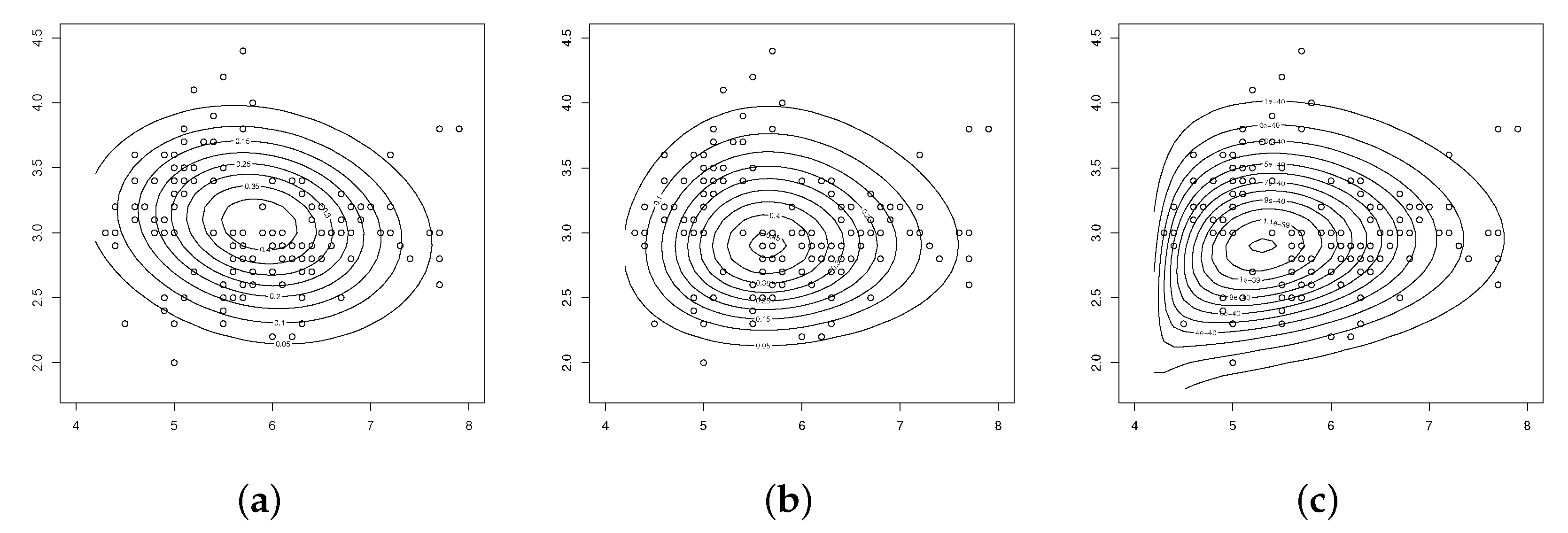
Table 3 presents ML estimates, AIC and CAIC values for BCSN, BPN and BPSN models, which is the one corresponding to the best (smallest AIC or CAIC) model fitting, which clearly indicates a better fit for BPSN model. Contour plots for the BPN, bivariate conditional skew-normal (BCSN) and BPSN distributions are presented in Figure 2.
Initially, the BPN model is compared to the BPSN model by the hypothesis tests
H 0 : ( λ 1 , λ 2 ) = ( 0 , 0 ) versus H 1 : ( λ 1 , λ 2 ) ( 0 , 0 ) .
by using the likelihood ratio statistic,
Λ = L BPN ( θ ^ ) L BPSN ( θ ^ )
where L BPN ( · ) and L BPSN ( · ) are the pseudo-likelihood function of the BPN ans BPSN model, respectively. We obtain
2 log ( Λ ) = 2 ( BPN ( θ ^ ) BPSN ( θ ^ ) ) = 6.704
which is greater than the value of the χ 2 , 95 % 2 = 5.99 . Then the BPSN model is a good alternative for fitting the data set. This result suggests the importance of the parameters λ 1 and λ 2 in the good fit of the BPSN model, the effect of these two parameters can be seen in the graph (c) of the Figure 2. The contour graphs in the Figure show that the BPSN model manages to better capture the distribution of the data set under consideration, since more points are contained within the contours of the BPSN distribution compared to the BCSN and BPN models.
Another hypothesis of special interest is the significance of the parameter vector ( α 1 , α 2 , α 12 ) , in this particular case there is interest in the hypothesis set
H 0 : ( α 1 , α 2 , α 12 ) = ( 1 , 1 , 0 ) versus H 1 : ( α 1 , α 2 , α 12 ) ( 1 , 1 , 0 )
So, under H 0 , we have the independent bivariate SN distribution for ( X 1 , X 2 ) . An appropriate test follows by using a statistic of type Wald which follows from the asymptotic normality of the maximum pseudo-likelihood estimator β ^ ̲ . This statistic can be defined as
W n = ( A β ^ ̲ m ) ( Σ ^ 3 ( β ^ ̲ ) ) 1 ( A β ^ ̲ m ) ,
where Σ ^ 3 ( β ^ ̲ ) is a submatrix of Σ ^ ( β ˜ ̲ ) corresponding to the vector ( α 1 , α 2 , α 12 ) , A = ( 0 3 × 6 I 3 ) and m = ( 1 , 1 , 0 ) , which, under the null hypothesis follows a χ 2 distribution with 3 degrees of freedom.
Thus, we obtained that W n = 1229.17 with p v a l u e = 0.0000 that is, the null hypothesis is rejected, indicating that the exponentiated component is significant in the model, thus, both components of the unification, skew and power, are significant in the good fit of the BPSN model.
The multivariate Kolmogorov-Smirnov test of goodness of fit proposed by [45], in special for the case of a bivariate distribution, which we denote by BKS (bivariate Kolmogorov-Smirnov), the statistic is given by
d n = sup ( x 1 , x 2 ) R 2 F n ( x 1 , x 2 ) F ( x 1 , x 2 )
where F n is the empirical distribution function of the sample, and F is some specified distribution function. When F distribution is unknown, the Kolmogorov-Smirnov statistic is defined by
d n ( F ) = max D 1 , D 2 ,
where
D 1 sup ( x 1 , x 2 ) R 2 G n ( y 1 , y 2 ) y 1 × y 2
by using the transformation y 1 = F X 1 ( x 1 ) and y 2 = F X 2 X 1 ( x 2 x 1 ) , and
D 2 sup ( x 1 , x 2 ) R 2 G n ( y 2 , y 1 ) y 2 × y 1
by using the transformation y 2 = F X 2 ( x 2 ) and y 1 = F X 1 X 2 ( x 1 x 2 ) , where G n is the empirical distribution function of the sample. For the special case of the BPSN model,
d n ( BPSN ) = max 0.05907079 , 0.07485913 = 0.07485913 ,
which is less than 0.1464 , which is the critical value of Table 1 given by [45], at level of 5%. Therefore, it is concluded that, the BPSN model fits well with the iris data set.
It should be noted that, the BPSN model is compared to other models, in particular a model of the skew-normal family of [1] proposed by [6], and a model of the power-normal family of [2] studied by [26]. Our proposal better fitted the data set studied in [35]. This allows us to conclude that the BPSN model is a viable alternative to those existing in the literature when the data set presents degrees of asymmetry that are not captured by the multivariate normal model.

4.2. Illustration 2

In the second application we use data on measurements on air-pollution variables recorded at 12:00 noon in the Los Angeles area on different days, available in [46]. For this application, we use the variables x = W i n d and y = N O 2 . For air pollutant concentrations, it is usually assumed that the data are uncorrelated and independent and thus do not require the diurnal or cyclic trend analysis [47]. The concentration of average air pollutants has been used in epidemiological surveillance as an indicator of the atmospheric contamination and its associated adverse effects in humans, causing diseases such as bronchitis.
The bivariate normality test of Royston returns a test statistic value of 13.55147 with p-value = 0.001141065, whereas the generalized Shapiro-Wilk test for multivariate normality returns a test statistic value of M V W = 0.94391 , with p-value = 0.01166 rejecting the hypothesis of normality of the observations vector. Thus, a model like the BPSN is an alternative to fit the vector of observations.
In this case, the maximum pseudo-likelihood estimates for the parameter vector is given by ξ ^ 1 = 5.8000 ( 0.3802 ) , ξ ^ 2 = 2.8274 ( 0.6279 ) , η ^ 1 = 4.9416 ( 0.5998 ) , η ^ 2 = 6.1694 ( 0.6590 ) , λ ^ 1 = 1.8609 ( 0.1185 ) , λ ^ 2 = 0.5184 ( 0.1263 ) , α ^ 1 = 10.14438 ( 5.0364124 ) , α ^ 2 = 11.3732 ( 6.5075 ) and α ^ 12 = 15.4635 ( 8.4410 ) .
For the hypothesis
H 0 : ( α 1 , α 2 , α 12 ) = ( 1 , 1 , 0 ) versus H 1 : ( α 1 , α 2 , α 12 ) ( 1 , 1 , 0 )
nosotros obtuvimos que W n = 196.6627 with p v a l u e = 0.0000 , es decir, se rechaza la hipótesis nula, indicando que la componente exponenciada es significativa en el modelo. For the The multivariate Kolmogorov-Smirnov test of goodness of fit,
d n ( BPSN ) = max { 0.1619804 , 0.1066137 } = 0.1619804 ,
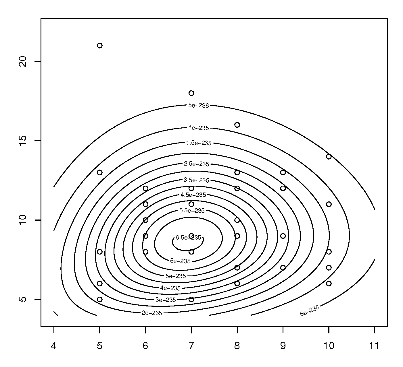
which is less than the values 0.2789 (for n = 40 ) and 0.2512 (for n = 50 ), then the BPSN model presents a good fit for the environmental pollution data in the city of Los Angeles. Contour plots for the bivariate PSN distributions is presented in Figure 3.

5. Concluding Remarks

In this article, on the basis of conditionally specified distributions, we have introduced a new bivariate PSE distribution which is very general, quite flexible and widely applicable. The new bivariate model is an absolutely continuous bivariate distribution whose marginals are univariate PSE distributions. We have derived several properties of the bivariate PSE distribution and special attention is centered in the particular case of de bivariate PSN distribution. The estimation of the unknown parameters of the new bivariate model is approached by using the proposal of [29] by maximization of the pseudo-likelihood function and the observed information matrix is determined. LR tests for some hypotheses of interest are also considered. As remarked, the new bivariate PSN model proposed in this article can be skewed and correlated, and therefore is much more flexible than other bivariate skew models available in the literature for analysing bivariate data. This is supported in the application to real data which is verified that the new bivariate PSN model provides consistently a better fit than the bivariate model proposed by [6].

Author Contributions

All authors contributed equally to this work. All authors have read and agreed to the published version of the manuscript.

Funding

The research of H. W. Gómez was supported by SEMILLERO UA-2020 project, Chile. The research of G. Martínez-Flórez was supported by project: Distribuições de Probabilidade Mutivariadas Assimétricas e Flexíveis, Universidade Federal de Ceará, Fortaleza, Brazil.

Conflicts of Interest

The authors declare no conflict of interest.

Appendix A

The elements of the K matrix can be written as:
κ ξ j ξ j = α 12 η j 2 i = 1 n z j i W ( 1 ) j i 2 π λ j W ( 3 ) j i + W ( 1 ) j i 2 [ α j α 12 ln ( F SN ( z j i ; λ j ) ) ] α 12 W ( 1 ) j i 2 [ α j α 12 ln ( F SN ( z j i ; λ j ) ) ] 2 1 η j 2 i = 1 n 1 + 2 π λ j 3 z j i W ( 2 ) j i + 2 λ j 2 π W ( 2 ) j i 2 1 η j 2 i = 1 n [ ( α j 1 ) 2 α 12 ln ( F SN ( z j i ; λ j ) ) ] z j i W ( 1 ) j i 2 π λ j W ( 3 ) j i + W ( 1 ) j i 2 ,
κ ξ j η j = α 12 η j 2 i = 1 n ( z j i 2 1 ) W ( 1 ) j i 2 π λ j z j i W ( 3 ) j i + z j i W ( 1 ) j i 2 [ α j α 12 ln ( F SN ( z j i ; λ j ) ) ] α 12 z j i W ( 1 ) j i 2 [ α j α 12 ln ( F SN ( z j i ; λ j ) ) ] 2 + 1 η j 2 i = 1 n 2 z j i + 2 π λ j ( 1 λ j 2 z j i 2 ) W ( 2 ) j i 2 λ j 2 z j i π W ( 2 ) j i 2 1 η j 2 i = 1 n [ ( α j 1 ) 2 α 12 ln ( F SN ( z j i ; λ j ) ) ] ( z j i 2 1 ) W ( 1 ) j i 2 π λ j z j i W ( 3 ) j i + z j i W ( 1 ) j i 2 ,
κ ξ j λ j = 2 π 1 1 + λ j 2 α 12 η j i = 1 n ( 1 + λ j 2 ) z j i W ( 3 ) j i + W ( 1 ) j i W ( 3 ) j i [ α j α 12 ln ( F SN ( z j i ; λ j ) ) ] α 12 W ( 1 ) j i W ( 3 ) j i [ α j α 12 ln ( F SN ( z j i ; λ j ) ) ] 2 + 1 η j 2 π i = 1 n ( λ j i 2 z j i 2 1 ) W ( 2 ) j i + 2 π λ j z j i W ( 2 ) j i 2 2 π 1 1 + λ j 2 1 η j i = 1 n [ ( α j 1 ) 2 α 12 ln ( F SN ( z j i ; λ j ) ) ] [ ( 1 + λ j 2 ) z j i W ( 3 ) j i + W ( 1 ) j i W ( 3 ) j i ] ,
κ ξ j α j = 1 η j i = 1 n α 12 [ α j α 12 ln ( F SN ( z j i ; λ j ) ) ] 2 + 1 W ( 1 ) j i ,
κ ξ j α 12 = 1 η j i = 1 n α j [ α j α 12 ln ( F SN ( z j i ; λ j ) ) ] 2 + 2 ln ( F SN ( z j i ; λ j ) ) W ( 1 ) j i ,
κ η j η j = α 12 η j 2 i = 1 n ( z j i 2 2 ) z j i W ( 1 ) j i 2 π λ j z j i 2 W ( 3 ) j i + z j i 2 W ( 1 ) j i 2 [ α j α 12 ln ( F SN ( z j i ; λ j ) ) ] α 12 z j i 2 W ( 1 ) j i 2 [ α j α 12 ln ( F SN ( z j i ; λ j ) ) ] 2 1 η j 2 i = 1 n 1 3 z j i 2 + 2 π λ j z j i ( 2 λ j 2 z j i 2 ) W ( 2 ) j i 2 π λ j 2 z j i 2 W ( 2 ) j i 2 1 η j 2 i = 1 n [ ( α j 1 ) 2 α 12 ln ( F SN ( z j i ; λ j ) ) ] ( z j i 2 2 ) z j i W ( 1 ) j i 2 π λ j z j i 2 W ( 3 ) j i + z j i 2 W ( 1 ) j i 2 ,
κ η j λ j = 2 π 1 1 + λ j 2 α 12 η j i = 1 n z j i 2 ( 1 + λ j 2 ) W ( 3 ) j i + z j i W ( 1 ) j i W ( 3 ) j i [ α j α 12 ln ( F SN ( z j i ; λ j ) ) ] α 12 z j i W ( 1 ) j i W ( 3 ) j i [ α j α 12 ln ( F SN ( z j i ; λ j ) ) ] 2 2 π 1 η j i = 1 n z j i W ( 2 ) j i 1 λ j 2 z j i 2 2 π λ j z j i W ( 2 ) j i 2 π 1 1 + λ j 2 1 η j i = 1 n [ ( α j 1 ) 2 α 12 ln ( F SN ( z j i ; λ j ) ) ] [ z j i 2 ( 1 + λ j 2 ) + z j i W ( 1 ) j i ] W ( 3 ) j i ,
κ η j α j = 1 η j i = 1 n α 12 z j i [ α j α 12 ln ( F SN ( z j i ; λ j ) ) ] 2 + z j i W ( 1 ) j i ,
κ η j α 12 = 1 η j i = 1 n α j z j i [ α j α 12 ln ( F SN ( z j i ; λ j ) ) ] 2 + 2 z j i ln ( F SN ( z j i ; λ j ) ) W ( 1 ) j i ,
κ λ j λ j = 2 π α 12 ( 1 + λ j 2 ) 2 i = 1 n λ j ( 1 + λ j 2 ) z j i 2 2 λ j + 2 π W ( 3 ) j i W ( 3 ) j i [ α j α 12 ln ( F SN ( z j i ; λ j ) ) ] 2 π α 12 W ( 3 ) j i 2 [ α j α 12 ln ( F SN ( z j i ; λ j ) ) ] 2 + 2 π i = 1 n λ j z j i 3 W ( 2 ) j i 2 π z j i 2 W ( 2 ) j i 2 2 π 1 ( 1 + λ j 2 ) 2 i = 1 n [ ( α j 1 ) 2 α 12 ln ( F SN ( z j i ; λ j ) ) ] λ j ( 1 + λ j 2 ) z j i 2 2 λ j + 2 π W ( 3 ) j i W ( 3 ) j i ,
κ λ j α j = 2 π 1 1 + λ j 2 i = 1 n α 12 [ α j α 12 ln ( F SN ( z j i ; λ j ) ) ] 2 + 1 W ( 3 ) j i ,
κ λ j α 12 = 2 π 1 1 + λ j 2 i = 1 n α j [ α j α 12 ln ( F SN ( z j i ; λ j ) ) ] 2 + 2 ln ( F SN ( z j i ; λ j ) ) W ( 3 ) j i ,
κ α j α j = i = 1 n 1 [ α j α 12 ln ( F SN ( z j i ; λ j ) ) ] 2 ,
κ α j α 12 = i = 1 n ln ( F SN ( z j i ; λ j ) ) [ α j α 12 ln ( F SN ( z j i ; λ j ) ) ] 2 ,
κ α 12 α 12 = i = 1 n j = 1 2 ln 2 ( F SN ( z j i ; λ j ) ) [ α j α 12 ln ( F SN ( z j i ; λ j ) ) ] 2 ,
κ α j α j = 0 , κ α j λ j = 0 , κ α j η j = 0 , κ α j ξ j = 0 ,
κ λ j λ j = 4 π α 12 ( 1 + λ j 2 ) ( 1 + λ j 2 ) i = 1 n W ( 3 ) j i W ( 3 ) j i ,
κ λ j η j = 2 2 π 1 η j α 12 1 + λ j 2 i = 1 n z j i W ( 3 ) j i W ( 1 ) j i ,
κ λ j ξ j = 2 2 π 1 η j α 12 1 + λ j 2 i = 1 n W ( 3 ) j i W ( 1 ) j i ,
κ η j η j = 2 α 12 η j η j i = 1 n z j i z j i W ( 1 ) j i W ( 1 ) j i ,
κ η j ξ j = 2 α 12 η j η j i = 1 n z j i W ( 1 ) j i W ( 1 ) j i ,
κ ξ j ξ j = 2 α 12 η j η j i = 1 n W ( 1 ) j i W ( 1 ) j i .

References

  1. Azzalini, A. A class of distributions which includes the normal ones. Scand. J. Stat. 1985, 12, 171–178. [Google Scholar]
  2. Durrans, S.R. Distributions of fractional order statistics in hydrology. Water Resour. Res. 1992, 28, 1649–1655. [Google Scholar] [CrossRef]
  3. Martínez-Flórez, G.; Bolfarine, H.; Gómez, H.W. Skew-normal alpha-power model. Statistics 2014, 48, 1414–1428. [Google Scholar] [CrossRef]
  4. Martínez-Flórez, G.; Bolfarine, H.; Gómez, Y.M.; Gómez, H.W. An Unification of Families of Birnbaum-Saunders Distributions with Applications. Rev. Stat. Stat. J. 2020. Available online: https://www.ine.pt/revstat/pdf/ANUNIFICATIONOFFAMILIESOFBIRNBAUM-SAUNDERS.pdf (accessed on 8 August 2020).
  5. Azzalini, A.; Dalla-Valle, A. The multivariate skew-normal distribution. Biometrika 1996, 83, 715–726. [Google Scholar] [CrossRef]
  6. Arnold, B.C.; Castillo, E.; Sarabia, J.M. Conditionally specified multivariate skewed distributions. Sankhya Indian J. Stat. Ser. A 2002, 64, 206–226. [Google Scholar]
  7. Arellano-Valle, R.; Bolfarine, H. On some characterizations of the T-Distribution. Stat. Probab. Lett. 1995, 25, 79–85. [Google Scholar] [CrossRef]
  8. Cambanis, S.; Huang, S.; Simons, G. On the theory of elliptically contoured distributions. J. Multivar. Anal. 1981, 11, 368–385. [Google Scholar] [CrossRef] [Green Version]
  9. Fang, K.T.; Kotz, S.; Ng, K.W. Symmetric Multivariate and Related Distributions, 3rd ed.; Chapman & Hall: London, UK, 1990. [Google Scholar]
  10. Gupta, A.K.; Varga, T. Elliptically Contoured Models in Statistics; Kluwer Academic Publishers: Boston, MA, USA, 1993. [Google Scholar]
  11. Kelker, D. Distribution theory of spherical distributions and location scale parameters generalization. Sankhya Indian J. Stat. Ser. A 1970, 32, 419–430. [Google Scholar]
  12. Azzalini, A.; Capitanio, A. Statistical applications of the multivariate skew normal distribution. J. R. Stat. Soc. Ser. B 1999, 61, 579–602. [Google Scholar] [CrossRef]
  13. Branco, M.D.; Dey, D.K. A general class of multivariate skew-elliptical distributions. J. Multivar. Anal. 2001, 79, 99–113. [Google Scholar] [CrossRef] [Green Version]
  14. Genton, M.G.; Loperfido, N.M. Generalized skew-elliptical distributions and their quadratic forms. Ann. Inst. Stat. Math. 2005, 57, 389–401. [Google Scholar] [CrossRef] [Green Version]
  15. Shushi, T. Generalized skew-elliptical distributions are closed under affine transformations. Stat. Probab. Lett. 2018, 134, 1–4. [Google Scholar] [CrossRef]
  16. Adcock, C.; Azzalini, A. A Selective Overview of Skew-Elliptical and Related Distributions and of Their Applications. Symmetry 2020, 12, 118. [Google Scholar] [CrossRef] [Green Version]
  17. Owen, D.B. Tables for computing bivariate normal probabilities. Ann. Math. Stat. 1956, 27, 1075–1090. [Google Scholar] [CrossRef]
  18. Johnson, N.L.; Kotz, S.; Balakrishnan, N. Continuous Univariate Distributions, 2nd ed.; Wiley-Blackwell; John Wiley & Sons: Hoboken, NJ, USA, 1995; Volume 2. [Google Scholar]
  19. Martínez-Flórez, G.; Pacheco, M.; Giraldo, R. Inference in log-alpha-power and log-skew-normal multivariate models. Commun. Stat. Theory Methods 2016, 45, 4397–4415. [Google Scholar] [CrossRef]
  20. Martínez-Flórez, G.; Farias, R.B.A.; Moreno-Arenas, G. Multivariate log-Birnbaum-Saunders regression models. Commun. Stat. Theory Methods 2017, 46, 10166–10178. [Google Scholar] [CrossRef]
  21. Martínez-Flórez, G.; Lemonte, A.J.; Salinas, H.S. Multivariate Skew-Power-Normal Distributions: Properties and Associated Inference. Symmetry 2019, 11, 1509. [Google Scholar] [CrossRef] [Green Version]
  22. Lemonte, A.J.; Martínez-Flórez, G.; Moreno-Arenas, G. Multivariate Birnbaum-Saunders distribution: Properties and associated inference. J. Stat. Comput. Simul. 2016, 85, 374–392. [Google Scholar] [CrossRef]
  23. Pljonkin, A.P. Features of the Photon Pulse Detection Algorithm in the Quantum Key Distribution System. In Proceedings of the 2017 International Conference on Cryptography, Security and Privacy, Goa, India, 15–17 December 2017; pp. 81–84. [Google Scholar]
  24. Pljonkin, A.P. Vulnerability of the Synchronization Process in the Quantum Key Distribution System. Int. J. Cloud Appl. Comput. 2019, 9, 50–58. [Google Scholar] [CrossRef] [Green Version]
  25. Arnold, B.C.; Castillo, E.; Sarabia, J.M. Conditionally specified distributions. In Lecture Notes in Statistics; Berger, J., Fienberg, J., Gani, J., Krickeberg, I., Singer, B., Eds.; Springer: New York, NY, USA, 1992; Volume 73. [Google Scholar]
  26. Martínez-Flórez, G.; Arnold, B.C.; Bolfarine, H.; Gómez, H.W. The multivariate alpha-power model. J. Stat. Plan. Inference 2013, 143, 1244–1255. [Google Scholar] [CrossRef]
  27. Arnold, B.C.; Strauss, D. Bivariate distributions with conditionals in prescribed exponential families. J. Roy. Stat. Soc. Ser. B 1991, 53, 365–375. [Google Scholar] [CrossRef]
  28. Arnold, B.C.; Castillo, E.; Sarabia, J.M. Conditionally Specification of Statistical Models; Springer Series in Statistics; Springer: New York, NY, USA, 1999. [Google Scholar]
  29. Besag, J. Statistical analysis of non-lattice data. J. Roy. Stat. Soc. Ser. D 1975, 24, 179–195. [Google Scholar] [CrossRef] [Green Version]
  30. Arnold, B.C.; Strauss, D. Pseudolikelihood Estimation: Some Examples. Sankhya Indian J. Stat. Ser. B 1991, 53, 233–2435. [Google Scholar]
  31. Cheng, C.; Riu, J. On Estimating Linear Relationships When Both Variables Are Subject to Heteroscedastic Measurement Errors. Technometrics 2006, 48, 511–519. [Google Scholar] [CrossRef]
  32. Rotnitziky, A.; Cox, D.R.; Bottai, M.; Robins, J. Likelihood-based inference with singular information matrix. Bernoulli 2000, 6, 243–284. [Google Scholar] [CrossRef]
  33. Salinas, H.S.; Gómez, H.W.; Martínez-Flórez, G.; Bolfarine, H. Skew-normal alpha-power model [Statistics 48(2014) 1414–1428]. Statistics 2018, 52, 950–953. [Google Scholar] [CrossRef]
  34. Azzalini, A.; Capitanio, A. The Skew-Normal and Related Families, 1st ed.; Cambridge University Press: Cambridge, UK, 2014. [Google Scholar]
  35. Fisher, R.A. The use of multiple measurements in taxonomic problems. Ann. Eugen. 1936, 7, 179–188. [Google Scholar] [CrossRef]
  36. Anderson, T.W.; Darling, D.A. A test of goodness of fit. J. Am. Stat. Assoc. 1954, 49, 765–769. [Google Scholar] [CrossRef]
  37. Doornik, J.A.; Hansen, H. An Omnibus Test for Univariate and Multivariate Normality. Oxf. Bull. Econ. Stat. 2008, 70, 927–939. [Google Scholar] [CrossRef]
  38. Henze, N.; Zirkler, B. A Class of Invariant Consistent Tests for Multivariate Normality. Commun. Stat. Theory Methods 1990, 19, 3595–3617. [Google Scholar] [CrossRef]
  39. Royston, J.P. Some Techniques for Assessing Multivarate Normality Based on the Shapiro-Wilk W. J. Roy. Stat. Soc. Ser. C 1983, 32, 121–133. [Google Scholar] [CrossRef]
  40. Royston, J.P. Remark AS R94: A Remark on Algorithm AS 181: The W-test for Normality. J. Roy. Stat. Soc. Ser. C 1995, 44, 547–551. [Google Scholar] [CrossRef]
  41. Akaike, H. A new look at statistical model identification. IEEE Trans. Autom. Contr. 1974, 19, 716–722. [Google Scholar] [CrossRef]
  42. Cavanaugh, J.E. Unifying the derivations for the Akaike and corrected Akaike information criteria. Stat. Probab. Lett. 1997, 33, 201–208. [Google Scholar] [CrossRef]
  43. R Development Core Team. R: A Language and Environment for Statistical Computing; R Foundation for Statistical Computing: Vienna, Austria, 2019; Available online: http://www.R-project.org (accessed on 10 January 2020).
  44. Pewsey, A. Problems of inference for Azzalini’s skew-normal distribution. J. Appl. Stat. 2000, 27, 859–870. [Google Scholar] [CrossRef]
  45. Justel, A.; Peña, D.; Zamar, Z. A multivariate Kolmogorov-Smirnov test of goodness of fit. Stat. Probab. Lett. 1997, 35, 251–259. [Google Scholar] [CrossRef] [Green Version]
  46. Johnson, R.A.; Wichern, D.W. Applied Multivariate Statistical Analysis, 6th ed.; Prentice Hall: Upper Saddle River, NJ, USA, 2007. [Google Scholar]
  47. Gokhale, S.; Khare, M. Statistical behavior of carbon monoxide from vehicular exhausts in urban environments. Environ. Model. Softw. 2007, 22, 526–535. [Google Scholar] [CrossRef]
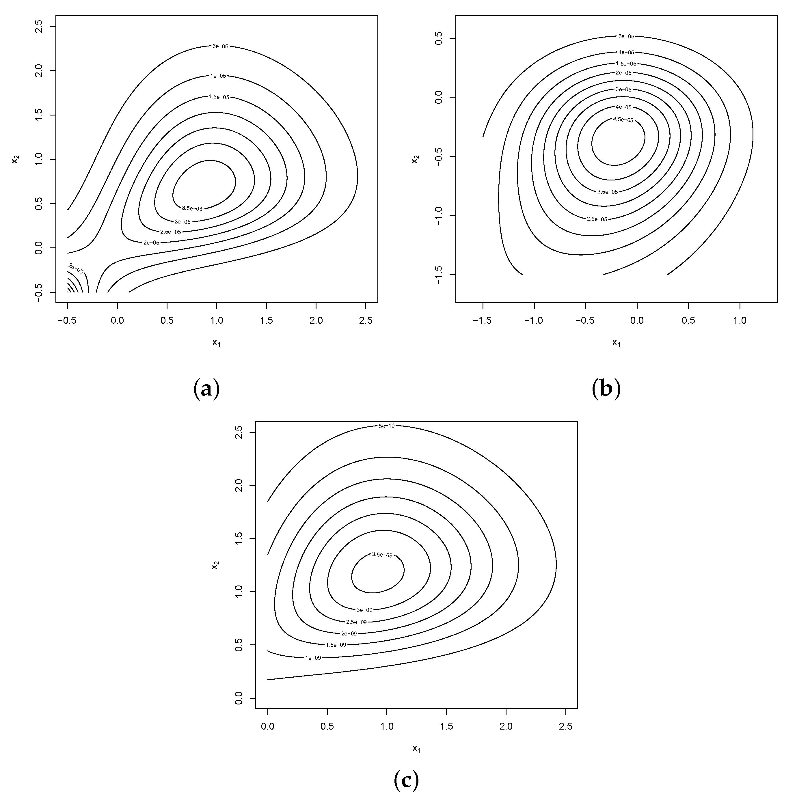
Figure 1. Graphs of contorns for the BPSN model (a) BPSN ((0,1), (0,1), 1.25, 2.75, 2.25, 1.75, 0.75), (b) BPSE ((0,1), (0,1), −1.25, −2.75, 2.25, 1.75, 0.75) and (c) BPSE ((0,1), (0,1), 1.25, 2.75, 2.25, 3.75, 1.25).
Symmetry 12 01327 g001
Figure 2. Contour plot of bivariate distributions for Iris data set: (a) BCSN model, (b) BPN model and (c) BPSN model.
Symmetry 12 01327 g002
Figure 3. Contour plots for the bivariate PSN distributions.
Symmetry 12 01327 g003
Table 1. Correlation coefficient for the BPSN distribution.
λ 2 / λ 1 −1.5−1.0−0.500.51.01.52.0
−2.50.80330.3730−0.2686−0.6699−0.8444−0.9252−0.9680−0.9933
−2.00.75180.3559−0.2385−0.6124−0.7759−0.8519−0.8924−0.9164
−1.50.60250.2984−0.1661−0.4625−0.5938−0.6556−0.6888−0.7087
−1.00.21050.1324−0.0046−0.1014−0.1479−0.1713−0.1845−0.1927
−0.5−0.2853−0.09210.17220.32450.38550.41170.42460.4317
0−0.5511−0.21900.25430.53850.65730.71050.73770.7534
0.5−0.6643−0.27560.28460.62440.76790.83270.86620.8856
1.0−0.7183−0.30350.29710.66310.81850.88880.92540.9467
1.5−0.7478−0.31930.30310.68340.84510.91860.95690.9791
2.0−0.7657−0.32910.30620.69510.86090.93620.97550.9985
2.5−0.7776−0.33580.30810.70260.87090.94760.98761.0000
Table 2. Summary statistics for the data set.
Variable x ¯ j s j b j 1 b j 2
x 1 5.8430.8280.308−0.605
x 2 3.0570.4350.3120.138
Table 3. Estimated parameters (standard errors), of the BCSN, BPN and BPSN models.
EstimateBCSNBPNBPSN
ξ ^ 1 5.867 (0.055)3.746 (0.136)4.119 (0.163)
ξ ^ 2 3.055 (0.035)1.655 (0.082)2.572 (0.159)
η ^ 1 0.794 (0.043)1.384 (0.058)1.417 (0.204)
η ^ 2 0.438 (0.026)0.808 (0.055)2.146 (0.390)
λ ^ 1 −0.224 (0.110) 11.147 (3.685)
λ ^ 2 −3.200 (0.504)
α ^ 1 9.358 (0.613)2.127 (0.192)
α ^ 2 14.746 (0.374)18.260 (3.158)
α ^ 12 2.671 (0.715)5.016 (1.473)
AIC555.10551.71549.00
CAIC557.68554.73552.59