Abstract
We propose a new approach to the model reduction of biochemical reaction networks governed by various types of enzyme kinetics rate laws with non-autocatalytic reactions, each of which can be reversible or irreversible. This method extends the approach for model reduction previously proposed by Rao et al. which proceeds by the step-wise reduction in the number of complexes by Kron reduction of the weighted Laplacian corresponding to the complex graph of the network. The main idea in the current manuscript is based on rewriting the mathematical model of a reaction network as a model of a network consisting of linkage classes that contain more than one reaction. It is done by joining certain distinct linkage classes into a single linkage class by using the conservation laws of the network. We show that this adjustment improves the extent of applicability of the method proposed by Rao et al. We automate the entire reduction procedure using Matlab. We test our automated model reduction to two real-life reaction networks, namely, a model of neural stem cell regulation and a model of hedgehog signaling pathway. We apply our reduction approach to meaningfully reduce the number of complexes in the complex graph corresponding to these networks. When the number of species’ concentrations in the model of neural stem cell regulation is reduced by 33.33%, the difference between the dynamics of the original model and the reduced model, quantified by an error integral, is only 4.85%. Likewise, when the number of species’ concentrations is reduced by 33.33% in the model of hedgehog signaling pathway, the difference between the dynamics of the original model and the reduced model is only 6.59%.
1. Introduction
A mathematical model of a chemical reaction network (CRN) can be represented by a system of ordinary differential equations (ODEs) that describe the dynamics of the concentrations of the constituent species participating in the network. Generally, kinetic models of most CRNs involve an immensely large number of variables, thereby making the models difficult to analyze due to the huge computational effort required for the analysis. On top of that, as in general not all of the species’ concentrations can be measured in an experimental set-up, identifying the parameters contained in the mathematical model is not feasible and demands massive experimental datasets. Thus, there exists a necessity to simplify the mathematical models of CRNs to reduced variants that preserve the key properties of the original models but contain fewer ordinary differential equations and fewer unknown variables. Numerous model reduction methods for CRNs are described in the literature. For a comprehensive survey of popular model reduction techniques, see, for example, in [1,2]. The quasi-steady-state approximation (QSSA) (see, for example, in ([3] Chapter 2) and ([4] Chapter 4)) is one of the most commonly used tools for model reduction of CRNs governed by enzyme kinetics. Even though QSSA can be used for a large variety of CRNs, in many cases it demands high computational efforts. The method is not simple to apply, as it requires a priori experimental (biological) knowledge.
A recent model reduction method proposed in [5] reduces the mathematical model of a CRN by eliminating complexes from its corresponding complex graph. In chemical reaction network theory, complexes are defined as the left- (substrate) and right-hand (product) sides of the reactions. Furthermore, the complexes of a CRN can be naturally associated with the vertices of a complex graph with edges corresponding to the reactions of the network. The method described in [5] selects the complexes to be eliminated in such a way that the behavior of the remaining relevant species in the reduced CRN is close to their original behavior. It is based on the Kron reduction method [6], and reduces the weighted Laplacian matrix associated with the complex graph. The Kron reduction method is a popular method of model reduction for electrical networks and proceeds by the computation of Schur complements [7] of the weighted Laplacian matrix. As an example, let us consider the following CRN consisting of a single linkage class,
where , , are distinct complexes and , , are the overall reaction rates in the forward direction. We recall from the work in [5] that a linkage class is a connected component of the complex graph corresponding to the CRN. After eliminating the complex using the method proposed in [5], we obtain the following reduced network.
Here, the principle of complex balancing is applied to to replace the two reversible reactions and of the original network by the new reversible reaction . We say that is complex balanced if its inflow is equal to its outflow. In other words, the concentrations of the species participating in are adjusted in such a way that , which leads to the deletion of from the complex graph. Moreover, the reaction rates , , of the other reactions remain unchanged. Note that the goal of considering this example is to illustrate how the reduction procedure in [5] is carried out. It describes how the aforementioned method is used to delete a complex (in this case the complex ) from the corresponding complex graph. Thus, without loss of generality, we assume that the deletion of does not cause major changes in the dynamics of the considered chemical reaction network.
This method is effective in eliminating intermediate complexes from linkage classes that have more than one reaction. We note that an intermediate complex is a complex participating in more than one reaction, with each reversible reaction considered as a single reaction. For instance, with reference to the network given above, is an intermediate complex, but is not. However, as mentioned in [5,8], when every linkage class has just two complexes, the method fails in producing a meaningful reduction as it just deletes reactions from the network. For example, consider the following part of a kinetic model of yeast glycolysis,
where is the overall rate of the jth reaction in the forward direction. Note that a reaction rate is a function of species’ concentrations of the network and it depends on the governing law of the corresponding reaction. In this case, elimination of any complex by the approach proposed in [5] results in deleting the corresponding reaction. For instance, if we delete the complex G6P + ADP from the network, the method will result in deleting the entire second reaction from the network. The reduced CRN will then have the reaction occurring independently of the remaining reactions. Therefore, the reduced network will possess a behavior that is completely different from the original one. It is easy to see that the complex graph corresponding to (1) is not connected. As this complex graph does not have any linkage class that contains more than one reaction, the method proposed in [5] does not result in a meaningful reduction of the corresponding model. In this case, there is a need to find a reasonable method of rewriting the complex graph of the given network as a graph with linkage classes that have more than one reaction in order to ensure that the application of the method proposed in [5] results in a meaningful reduction in the number of complexes.
We propose to eliminate the species ADP from the network in such a way that we can replace the reactions and with the reversible reactions Glci + ATP ⇄ G6P and F6P + ATP ⇄ F16BP, respectively. This replacement can be done, for example, by expressing the concentration of ADP in terms of the concentrations of ATP. This can be done by using the two ODEs that represent the change in concentration over time for ADP and ATP. These ODEs can be represented in the following form,
where denotes the molar concentration of the species X. From these equations, we easily derive the following conservation law, which express the concentrations of ADP in terms of the concentration of ATP,
where C is a non-negative constant (known as a conserved quantity) depending on the initial concentrations of ATP and ADP. The conservation law (2) can now be used to eliminate the concentration of the species ADP from the mathematical model of the network. This elimination allows us to rewrite the mathematical model as a model of a network containing two linkage classes that consist of more than one reaction.
Note that even though the species ADP is not explicitly participating anymore in the CRN, its concentration still appears in the corresponding mathematical model in terms of the concentration of ATP. The method in [5] may now be used on the network (3) to reduce its mathematical model in a meaningful way by deleting the species (complexes) G6P and F16BP from the corresponding complex graph. Even though the elimination of the concentration of ADP enables the application of the reduction method [5], the reduced model is valid only for trajectories for which the total concentration of the pool of ADP and ATP is fixed.
Most CRNs in real-life have reaction network structures similar to the original yeast glycolysis network (1), with certain linkage classes consisting of only one reaction. New tools for model reduction are required for these types of networks. In this paper, we generalize the approach of the complex graph rewriting procedure briefly illustrated above. This procedure, in conjunction with the method proposed in [5], results in a meaningful model reduction.
The main idea of our model reduction method is to enable the application of the model reduction method proposed in [5] by joining certain linkage classes of a CRN into a single linkage class using linearly independent conservation laws. An important result related to conservation laws is Noether’s theorem [9], which states that there is a one-to-one correspondence between a conservation law and a differentiable symmetry of nature. For instance, an example of a conservation law in the field of classical physics is the law of conservation of energy in Hamiltonian systems, which corresponds to time translation symmetry.
We develop an automation process for our model reduction method in order to make it straightforward to apply for a wide range of CRNs governed by any kind of enzyme kinetics. In the automation procedure we assume that the CRN admits a single steady state and is asymptotically stable around it. This assumption is necessary for determining the settling time of the network over which we compare the original model and the reduced model. We created a MATLAB library, which contains all the files corresponding to each step of our step-wise reduction procedure. It uses the input files containing the information of a given CRN provided by the user to reduce the corresponding mathematical model in a fully automated fashion.
Finally, we exhibit the application of our new technique of model reduction for real-life examples of CRNs drawn from the Biomodels database [10]. For each of the cases, we explain how the corresponding mathematical model can be meaningfully reduced.
2. Preliminaries
In this section, we give a compact description of the mathematical techniques that are necessary for our automated model identification method. We commence by introducing the notations that are used throughout the manuscript and continue by explaining a framework for deriving a system of ODEs that describes the dynamics of the constituent species of a given CRN. Subsequently, we recall the Kron reduction method proposed in [5].
denotes a reaction from the substrate to the product , where the dotted line indicates that it can be reversible or irreversible. In this case, when referring to its reaction rate we refer to the outgoing overall reaction rate in the forward direction. The transpose and the null space of an matrix , , , are denoted by and , respectively. The number of elements of a set I is denoted by . For any vector , denote by the diagonal matrix whose diagonal elements are the corresponding elements of the vector v. Define the function as and the function as . The Schur complement of the block matrix of the matrix is denoted by .
2.1. Mathematical Models of Reaction Networks
Consider a CRN that involves m distinct chemical species, c complexes, and has r unidirectional reactions. We present a framework for describing the dynamics of reaction networks using their complex graphs [5,11]. The c complexes of the network are represented by an complex composition matrix Z, whose columns express the complexes in terms of their species. Any CRN is defined by a incidence matrix B, where
It can be shown that the stoichiometric matrix S of the network is . We denote by the vector of reaction rates of the given CRN. The basic structure underlying the dynamics of the species’ concentration vector is given by the balance law [12]:
Let . Using (4) we easily see that this vector satisfies the condition . Consequently, is a constant, and thus
where is the vector of initial species’ concentrations, i.e., . Equation (5) is called a conservation law of the CRN. The constant term appearing in the conservation law (5) is called a conserved quantity. Clearly, the number of linearly independent conservation laws is equal to the dimension of . In other words, irrespective of the governing laws, we can obtain a maximal set of linearly independent conservation laws by computing .
Let be the column of Z corresponding to the substrate of the ith reaction. Assuming that every reaction of the CRN is governed by an enzyme kinetic rate law, the reaction rate of the ith unidirectional reaction between the substrate and product , as explained in [5], can be expressed as
where, for every , is a rational function and denotes the rate constant of the ith reaction. Note that if the governing law of the ith reaction is mass action kinetics, then . Consider the diagonal matrices and . Define the outgoing matrix as follows,
It can be shown that the weighted Laplacian matrix associated with the complex graph of the network is . As explained in [5], the balance laws (4) can be expressed in terms of the Laplacian matrix as
where . Some well-known enzyme kinetic rate laws for which the balance laws can be written in matrix multiplication form (7) are the reversible Michaelis–Menten kinetics [13], Monod–Wyman–Changeaux kinetics [14], Hill kinetics [15,16], Ping Pong Bi Bi kinetics [17], and Koshland–Nemety–Filmer kinetics [18]. In order to clearly illustrate the modeling procedure, we demonstrate it for the following reaction network with four unidirectional reactions,
where ∅ is the zero complex representing the environment. It is treated as a regular complex, in which the number of moles of each species is zero as explained in [11]. More precisely, the first reaction is a creation of and the last reaction is a degradation of . In this example, the substrate complexes of the four reactions are , , , and , respectively. Thus, , , , and . The complex composition matrix and the incidence matrix corresponding to the network (8) are given by
Let and be the maximum reaction rates of the second and the third reactions of (8), respectively. The expressions for the reaction rates (6) depend on the governing laws of the reactions. One possibility is
where is the Michaelis constant of the species for , and , are positive constants. The reaction rates of the network (8) can be represented in the form (6) by defining the rate constants as
and the rational terms in the expressions of reaction rates as
The Laplacian matrix corresponding to the network (8) is
Note that open CRNs are modeled in [5] by extended balance laws of the form , where the free term represents the inflows to and outflows from the complexes of the network. Here, as the zero complex is considered as a regular complex it is included in the Laplacian matrix in order to avoid the unnecessary free term. On top of that, unlike the reduction method proposed in [5], if the zero complex is an intermediate complex, we consider it as a candidate complex for deletion.
2.2. Kron Reduction of Mathematical Models Corresponding to Reaction Networks
We describe the model reduction method proposed in [5]. It is based on the Kron reduction [6] and is performed by deleting a set of complexes from the complex graph associated with the CRN. Recall that deleting a complex is equivalent to assuming that it is complex balanced. The complex balancing is carried out by computing the Schur complement [7] of the weighted Laplacian matrix associated with the corresponding complex graph.
Definition 1.
Let L be an block matrix of the form
where A, B, C, and D are , , , and matrices, respectively. Assume that D is invertible. The Schur complement of D is the matrix defined by
Consider again a CRN of c complexes and r reactions with dynamics modeled by the balance laws (7). Let V be the set of indices corresponding to the complexes of the CRN, i.e., . Assume that we want to delete the complexes with the set of indices , which is a subset of V of cardinality] . Denote by the block matrix of the Laplacian matrix that corresponds to the set of indices . The complex deletion is carried out by computing the Schur complement (see, for example, in [7]) of the block matrix . It is proven (see in [5] Proposition 1) that is again a Laplacian matrix, i.e., it satisfies the properties of Laplacian matrices [19]. On top of that, it is shown that the equation
describes the dynamics of a CRN governed by an enzyme kinetics rate law, i.e., the corresponding reaction rates can be written in the form (6), with smaller number of complexes. Here, is the complex composition matrix of the reduced CRN defined by removing from Z the columns corresponding to the set of indices . A suitable choice of ensures that some of the elements in the vector of species concentrations x are conserved in time, i.e., the derivatives of some of the elements of x are zeros. This leads to a reduced number of dependent variables in the corresponding mathematical model. As an example consider the following simple CRN of two unidirectional reactions,
Let and be the overall rates in the forward direction of the first reaction and the second reaction, respectively. For , denote by the concentration of the species . In this case, the balance laws (4) can be rewritten as
Now suppose that the second complex is complex balanced, which is equivalent to assuming that . From the above-mentioned balance laws we obtain , which means that and are conserved in time.
In [5], the difference between the dynamical behaviors of the original model and the corresponding reduced model is quantified by an error integral E. Let be the time interval over which we want to observe the difference between the behaviors of the original model and the reduced model. Denote by J the set of indices of the significant species of the network. The error integral E is defined as
where and are the concentrations of the ith species in the original model and the reduced model, respectively. Note that in [5] the right endpoint of the time interval has been set manually. However, in our case this right endpoint is chosen to be the settling time of the network, i.e., the time instant at which the considered CRN reaches a sufficiently small prespecified neighborhood of its unique steady state.
The model reduction method proposed in [5] is an iterative procedure that selects a subset of intermediate complexes to be deleted from the corresponding complex graph as follows. First, the candidate complexes for deletion, i.e., the intermediate complexes of the network, are identified. For each candidate complex the error integral corresponding to the reduced model obtained after its deletion is evaluated. These values of error integrals are used to rank the candidate complexes and then delete the candidate complex with the least value of error integral. In the next step, the above-mentioned procedure is repeated with the reduced model. The iteration is continued until the error integral exceeds a prespecified threshold value.
One of the advantages of the reduction method [5] is that it does not rely on a priori biological knowledge about the CRN. Moreover, it is an easy-to-implement model reduction method that can be used to simplify huge mathematical models of CRNs by retaining the original kinetics.
3. Equivalent Mathematical Models
In this section, we give a detailed explanation of the basic idea of our reduction technique which we briefly introduced in Section 1. We first establish concepts that are relevant to the model reduction procedure.
Definition 2.
Theindex set, , corresponding to the complex of the network, is the set of indices of the species participating in the expression of the complex .
We thus obtain the following expression for the complex in terms of its species,
where represents the number of moles of the ith species in the expression of the complex . It is clear that two complexes and share common species if and only if . Trivially, .
Definition 3.
Let be a complex of a CRN. For , we define as the new complex consisting of the species of with their respective number of moles multiplied by ε, i.e., .
With the following lemma, we show the equivalence between two mathematical models of a given CRN. Later on, we will see that the application of this lemma allows us to join certain reactions into a single linkage class.
Lemma 1.
Let be the vector of overall reaction fluxes in the forward direction of the CRN , . For every , the reaction network is equivalent, in terms of its mathematical model, to the reaction network , , with the vector of overall reaction fluxes being .
Proof.
Let , be a random species of the CRN , . Using (4), the rate of change of the concentration of species is given by
As the right-hand side of this equation represents the rate of concentration change of species in the original network, the proof of Lemma 1 is complete. □
Remark 1.
As the CRNs , , with , and , , with , have the same mathematical models, they also possess the same conservation laws.
In the following proposition, we generalize the idea of the complex graph rewriting procedure, as was roughly illustrated in Section 1. We show that in the presence of a shared species between two complexes, a suitable conservation law can be used to join the corresponding reactions with the shared species as intermediate complexes.
Proposition 1.
Let be the vector of overall reaction rates in the forward direction of the CRN , . Suppose that, for certain , two complexes, and , of different reactions share a common species , . Define , where and are the sets of indices corresponding to the complexes and , respectively. If for every , there exists a conservation law in which the species is participating, but not the remaining species corresponding to I, then we can join the two reactions, and , into a single linkage class ,
with the corresponding reaction rates being
The intermediate complex is the shared species with number of moles , i.e., .
Proof.
For every , choose a vector such that the corresponding conservation law (5) satisfies the assumptions of the proposition. Note that this vector strictly depends on . More precisely, its th component is not equal to zero. Moreover, note that all the other components of corresponding to I are zeros. Denote by the vector with its th element replaced by zero. Using (5) we represent in terms of the concentrations of the other species:
where is the vector of species’ initial concentrations. By substituting as in the above equation in the expression of the vector of the reaction rates, we can rewrite the reactions , , in the following forms
Application of Lemma 1 with
completes the proof. □
As (10) represents a linkage class with more than one reaction, the method proposed in [5] can be meaningfully applied to delete the intermediate complex from the corresponding complex graph. In the reduced network, the linkage class (10) can be replaced by a single reaction using the principle of complex balancing.
Remark 2.
We would like to point out the three major steps of the complex graph rewriting procedure described in the proof of Proposition 1. Later on, these steps will be used to automate our model reduction procedure.
- M1.
- Elimination of certain species from the network (rewriting the corresponding concentrations in terms of the concentrations of the other species), after which certain complexes are composed of the same species.
- M2.
- Application of Lemma 1 in order to make such complexes identical to each other.
- M3.
- Joining the reactions with identical complexes into a single linkage class.
4. Automatic Reduction Procedure
In this section, we describe the automatic model reduction procedure step by step. We show how to apply Proposition 1 for any kind of CRN independently of its governing laws to join certain reactions in an automatic way. We then apply the strategy in [5] to reduce the number of complexes in the complex graph corresponding to the equivalent network.
Inputs: The list of inputs required for the model reduction procedure is as follows.
- The complex composition matrix , where m and c are the number of the species and complexes of the network, respectively.
- The incidence matrix of the network, where r is the number of reactions of the network.
- The vector of rate constants of the reactions.
- The vector of rational terms in the expressions of reaction rates.
- The vector of initial concentrations.
- The threshold value of the error integral (9), i.e., the maximum admissible value of E.
Outputs: The automatic reduction procedure provides the following outputs.
- The mathematical model and the complex graph corresponding to the original network.
- The mathematical model and the complex graph corresponding to the reduced network.
- The final value of the error integral.
We divide our model reduction procedure into seven steps. In order to clearly explain the reduction procedure throughout this section, we will demonstrate it step by step for the following example of six unidirectional reactions:
with the corresponding reaction rates being
- Step 1: Mathematical model of the network.
In the first step, we determine the system of differential Equation (7) that underlies the dynamics of the species’ concentration vector .
- Step 2: Settling time of the network.
Each CRN is uniquely described by the system (7) obtained from its structure. We can then commence considering its model reduction. An important tool, which is crucial in our reduction procedure, is the settling time of the considered CRN defined in Section 2.2. We show how to automatically compute it for a given CRN.
It has been proved in [20] that for a class of networks called zero deficiency networks, there exists a unique point satisfying the following system,
where , , form a maximal set of linearly independent conservation laws. In [11,21,22], the same result has been proved for a related class of networks called complex balanced networks. It states that such a network is asymptotically stable around its unique steady state corresponding to a particular initial concentration . We assume that the same property is true for the CRNs considered for our reduction procedure as mentioned in the introduction. Solving the system (13), we find the unique steady state . The settling time of the CRN can then be automatically computed by the so called bound function defined as follows. For a fixed , the -bound function is given as
Note that the bound function is computed component-wise. For an appropriate choice of , it is an easy numerical task to find the vector of settling time, such that , , is the time when the bound function corresponding to the ith species becomes 1 and remains so.
- Step 3: Selecting species to be eliminated from the network.
Next, we identify the set I of indices corresponding to the species whose elimination from the network results in joining certain reactions. This can be done by using the index sets , , corresponding to the complexes of the network, which can be easily extracted from the complex composition matrix Z. For a given pair of complexes and that share at least one species , define . If and share no species, set . It is reasonable to define the set I of indices to be eliminated from the network as . We note that if there exists a complex , which is made up of a single species with , i.e., , the elimination of from the network will end up eliminating the entire complex , meaning that becomes the zero complex.
The above-mentioned procedure allows us to determine the set of indices I in a fully automated manner. For example, in the case of the network (12), we obtain .
- Step 4: Mathematical model of the equivalent network.
In this step, we show how to determine the mathematical model of the equivalent network obtained after eliminating the species corresponding to I from the original network. For every , we find the corresponding conservation law that can be used with Proposition 1 to eliminate the concentration from the mathematical model of the original network. It can be done by computing , where is the matrix obtained by replacing all the rows of the stoichiometric matrix S that correspond to the elements of , with zero rows. If the assumptions of Proposition 1 are satisfied, then it can be used to join certain reactions. The mathematical model of the equivalent network is then determined according to the steps described in Remark 2. We give a detailed explanation of how Z, B, k, d, and for the corresponding model change after each step.
- M1.
- As the eliminated species are no longer participating in the equivalent network, we delete the corresponding rows from Z. Subsequently, the vector of species’ concentrations is defined by deleting the th, , element of x. Similarly, we obtain the vector of initial concentrations of the equivalent network. The vector of the rational functions can be derived from in the following way. For every , if the species is participating in the substrate complex of jth reaction, then , which ensures that the reaction fluxes of the network obtained at this step still obey the Equation (6). For the network (12), it is clear that the species is participating in the substrate complex of the second reaction. After rewriting the concentration function in terms of concentrations of the other species, we multiply by . Thus, . Similarly, we have , , and . We therefore write the reactions of the network (12) in the following form.
- M2.
- After the elimination of species, the columns of Z corresponding to the complexes that share species become multiples of each other. Consequently, in order to make these columns identical to each other, we multiply each of them by the corresponding constant from (11). Likewise, we divide each rate constant by the corresponding constant given in (11). In the case of the network (12), the vector of rate constants of its corresponding equivalent network is . We therefore rewrite the reactions (14) in the following form.
- M3.
- We now delete the duplicate columns of Z and keep only one of them in order to find the complex composition matrix of the equivalent network. Suppose that , where and are the number of species and complexes in the equivalent model, respectively. It is clear that, if and the number of duplicate columns is , then and .Let the pth and qth complexes be a pair of identical complexes. We first replace the pthrow of B withand delete its qth row. We then repeat the same technique for all the pairs of identical complexes to obtain the incidence matrix of the equivalent network. It is clear that .The complex composition matrix and the incidence matrix of the equivalent network corresponding to the network (12) are
Thus, the equivalent network corresponding to the network (12) becomes
Define , where is the vector of rate constants of the equivalent network. Then, the Laplacian matrix of the equivalent network is , where and is the outgoing matrix of the equivalent network. The mathematical model of the equivalent network is
where .
- Step 5: Independent subnetworks.
In some cases, the equivalent network may consist of independent subnetworks, which contain sets of reactions that do not share any common species. In this situation, we determine all the independent subnetworks of the equivalent network. First, we determine the linkage classes of the equivalent network using its incidence matrix . The index sets corresponding to the complexes of the equivalent network are then used to determine the indices of the species participating in each linkage class. More precisely, if , are the complexes of the same linkage class , then the set of indices of is . It is clear that two linkage classes and are dependent, if . Mutually dependent linkage classes form an independent subnetwork of the equivalent network.
Let , , be the independent subnetworks of a network having more than one reaction. As they are independent, we can consider each of them as a separate network. Thus, we consider the reduction of each of them separately. We note that in the case of the network (12), there is only one subnetwork in the corresponding equivalent network.
- Step 6: Selecting complexes for deletion.
In this step, we apply the reduction procedure of [5] to meaningfully delete certain complexes from the equivalent network. The first step of this procedure is to determine the candidate (intermediate) complexes for deletion. We note that the intermediate complexes are the ones that participate in more than one reaction, with each reversible reaction considered as a single reaction. It is reasonable to consider all the other complexes as important complexes. We consider the constituent species of the important complexes as the important species. In [5], the candidate complexes for deletion have been chosen manually. Here, we show how to determine such complexes in an automatic way. Let be the incidence matrix of the equivalent network, with each reversible reaction considered as a single reaction. can be found by deleting the columns of corresponding to the reverse reactions of reversible reactions. The intermediate complexes can then be determined from by detecting the rows that contain more than one nonzero element.
In the case of the network (15), we have
The candidate complexes for deletion from the linkage class (15) are and . The important species are , , , and , which are the constituent species of the important complexes and .
Let be the set of indices of the important species of . As explained in [5], we rank the candidate (intermediate) complexes according to the error integral defined in (9). Here, is the settling time of . We delete from the optimal combination of complexes, i.e., the combination with the maximum value of that does not exceed the predefined threshold.
- Step 7: Mathematical model of the reduced network.
Let be the set of indices of complexes deleted from , . Define . In the final step, we show how to determine the mathematical model of the reduced network after deleting the complexes with indices from the equivalent network. In order to obtain the complex composition matrix of the reduced network, we delete the columns of corresponding to . Define , which is the set of indices corresponding to the complexes remaining in the reduced network. According to Proposition 1 in [5], the Laplacian matrix of the reduced network is defined as the Schur complement of corresponding to . The mathematical model of the reduced network is then given by
where .
5. Application to Real-Life Reaction Networks
In this section, we apply our automatic model reduction method to reduce two computational models of biological processes that consist of several linkage classes, with common species shared between at least two of them. These models have been retrieved from the BioModels database [10], which is a repository of computational models of biological processes available online at https://www.ebi.ac.uk/biomodels/. For both models considered throughout this section, the threshold value of the error integral for stopping the iterative reduction procedure has been set to 0.15. In general, this threshold can be chosen depending on the desired closeness of the reduced model to the original model. Detailed explanations of the reduction procedure of these models are provided in Appendix A.
5.1. Neural Stem Cell Regulation
We consider a mathematical model of neural stem cell regulation (NSCR). The complex graph corresponding to the model is given in the left-hand panel of Figure 1. For the corresponding detailed mathematical model we refer to [23]. The concentrations of the important species participating in the original model are represented in Figure 2.
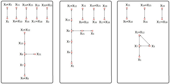
Figure 1.
The left-hand panel is the complex graph corresponding to the original model of neural stem cell regulation. The complex graph corresponding to the equivalent model obtained after eliminating the species , , and from the original model is given in the middle panel. Deletion of the intermediate complexes , , , and leads to a reduced network with the corresponding complex graph represented in the right-hand panel. The difference between the original model and the reduced model, as measured by the error integral, is 4.85%.
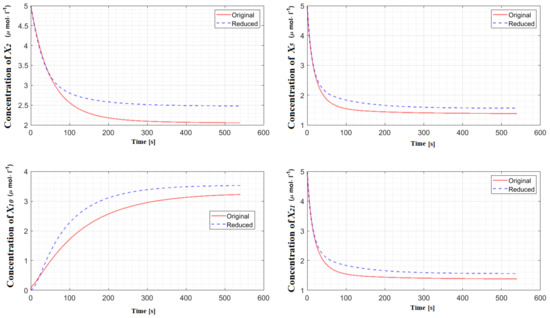
Figure 2.
Concentrations of the important species of neural stem cell regulation in the original model and in the reduced model. The difference between these models, as measured by the error integral, is 4.85%.
We note that there is one linkage class with more than one reversible reaction. The remaining linkage classes of the network contain only one reversible reaction. In this case, the method proposed in [5] can be meaningfully applied to delete the intermediate complexes , , and . Further reduction of the network using the same method would eliminate reactions from the network. To overcome this shortcoming and to obtain a meaningful model reduction of the network, we apply our new reduction technique.
Step 3 of our reduction procedure selects the species , , and to be eliminated from the mathematical model, which allows us to join three linkage classes into a single one. Detailed explanation of the elimination procedure can be found in Appendix A.1. In particular, we use three conservation laws to complete the aforementioned elimination of species. However, as a downside of our elimination procedure, the obtained reduced model is valid only for trajectories for which the three conserved quantities have fixed values as in (A2). For example, the first of these three conserved quantities is the total concentration of the pool of Notch [24] and Notch transmembrane [25], and it is reasonable to assume that in an experimental set-up this pool has a fixed concentration. The complex graph corresponding to the equivalent network of NSCR is shown in the middle panel of Figure 1.
Finally, applying the procedure described in Step 6 to this equivalent network, we delete the optimal combination of the intermediate complexes, which consists of , , , and . The complex graph corresponding to the reduced network is given in the right-hand panel of Figure 1. Even though 33.33% of the species have been deleted from the original model, the error integral is only 4.85%. The concentrations of the important species participating in the reduced model are represented in Figure 2.
5.2. Hedgehog Signaling Pathway
Subsequently, we have used our new technique of model reduction to a very different type of biochemical reaction network, namely, a model of hedgehog signaling pathway (HSP). The corresponding detailed mathematical model can be found in [23].
There are nine reversible and two irreversible reactions in the original network. The complex graph corresponding to the original network is given in the left-hand panel of Figure 3. The concentrations of the important species participating in the original model are represented in Figure 4. We observe that it contains two linkage classes consisting of more than one reaction. The remaining six linkage classes consist of only one reversible reaction. In this case, the reduction method proposed in [5] can be meaningfully applied to delete four intermediate complexes, namely, , , , and . Further reduction using the same procedure would lead to the deletion of reactions, which is not desirable in the sense of preserving the original behavior. However, the use of our new approach results in a meaningful reduction without causing a significant change in the original behavior. Detailed explanation of the species elimination procedure is included in Appendix A.2.
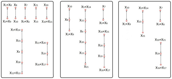
Figure 3.
The left-hand panel is the complex graph of the original model of hedgehog signaling pathway. The complex graph corresponding to the equivalent model obtained after eliminating the species , , and from the original model is given in the middle panel. Deletion of the intermediate complexes , , , and leads to a reduced model with the corresponding complex graph shown in the right-hand panel. The difference between the original model and the reduced model, as measured by the error integral, is 6.59%.
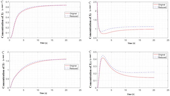
Figure 4.
Concentrations of the important species of hedgehog signaling pathway in the original model and in the reduced model. The difference between these models, as measured by the error integral, is 6.59%.
Step 3 of our reduction procedure chooses the species , , and to be eliminated from the network, i.e., . Similar to the model of NSCR, we use three conservation laws to eliminate these species. Again, as a downside of our reduction procedure, our final reduced model of HSP is valid only for trajectories for which the three conserved quantities have fixed values given by (A6). For example, the first of these conserved quantities is the total concentration of the pool of ADP (adenosine diphosphate) and ATP (adenosine triphosphate), and it is reasonable to assume that in an experimental set-up this pool has a fixed concentration.The complex graph corresponding to the equivalent network is shown in the middle panel of Figure 3.
Finally, the procedure described in Step 6 results in , , , and to be the optimal combination of the intermediate complexes for deletion, i.e., the maximal combination of complexes with an error integral of at most 15%. Deletion of these complexes by the procedure of [5] leads to the reduced network with the corresponding complex graph given in right-hand panel of Figure 3. We remark that, even though 33.33% of the species have been eliminated from the model, the resulting error integral is only 6.59%. The concentrations of the important species participating in the reduced model are represented in Figure 4.
6. Conclusions and Discussion
In this paper, we have illustrated a new approach to the model reduction of CRNs, which extends the method proposed in [5]. Our method is based on eliminating concentrations of certain species from the mathematical model corresponding to the network using the conservation laws obtained from the model. This elimination allows us to rewrite the complex graph of the network in a preferred form, for which the model reduction method proposed in [5] becomes meaningfully applicable. Even though the procedure results in reducing the order of the corresponding mathematical model, new parameters depending on the vector of initial concentrations are added to the model.
We have implemented an automated process for our model reduction method, which is divided into seven steps. We created a MATLAB file corresponding to each step and all files are included in a single MATLAB library. The information of a given CRN is provided by the user and subsequently used to reduce the corresponding mathematical model in a fully automated manner. The error integral defined in [5] is used to measure the difference between the behaviors of the original model and the reduced model. An important tool in the definition of the error integral is the settling time of the network, which was computed manually in [5]. We have shown how to automatically determine the settling time of a given CRN using its steady state. We have also been able to determine the intermediate complexes in a fully automated manner using the incidence matrix of the network. The MATLAB library consisting of all the files corresponding to our step-wise reduction procedure is provided as Supplementary Materials.
We have successfully applied our model reduction method on two real-life examples: neural stem cell regulation and the hedgehog signaling pathway. For each case, we have used our techniques to enable the reduction method proposed in [5] to be applied to a significant extent. We have been able to automatically join several linkage classes of the network by eliminating concentrations of certain species from the corresponding mathematical model. Table 1 provides the percentage of deleted species and the value of the corresponding error integral for each reaction network. The detailed explanation of the reduction procedure corresponding to these models can be found in the Supplementary Materials.

Table 1.
The amount of deleted species and the value of the error integral (in%) corresponding to each example after its model reduction using our method.
The major tools in our automated reduction method are the linearly independent conservation laws, which are used to eliminate the concentrations of species with index set I from the network. The identification of the set I is straightforward. However, in some cases, not all the selected species can be eliminated from the network because of the lack of suitable conservation laws, i.e, in the case when the number of the linearly independent conservation laws is less than the number of elements in I. In such cases, we select I in a way that the number of its elements is equal to the number of linearly independent conservation laws of the network. This adjustment ensures that the species with index set I can be eliminated from the network. Note that, even though this elimination rewrites the complex graph of the network in a preferred form (i.e., increases the number of intermediate complexes in it), new parameters (conserved quantities) are added in the corresponding mathematical model.
Although the procedure of elimination of species using conservation laws described in this paper improves the extent of applicability of the model reduction method in [5], it is no longer valid for all trajectories of the original model. As mentioned earlier, the reduced model is valid only for trajectories with fixed values of these conserved quantities. This aspect is similar to the case of the Michaelis–Menten approximation of enzyme kinetic networks which depends on a conserved quantity, namely, the total enzyme concentration.
One of the main advantages of the model reduction procedure proposed in [5] is that it preserves the governing laws of the CRN. For instance, if a CRN is governed by Michaelis–Menten kinetics, then the reduced CRN by the approach in [5] will again be governed by Michaelis–Menten kinetics. However, this is not the case for our automatic reduction method due to the rewriting procedure, as we have explained in [8].
In [5], the behaviors of the species’ concentrations participating in the reduced model are compared with the ones participating in the original model using the error integral (9) defined over a manually set timescale. In this paper, the same procedure has been adopted with the significant modification that the time length of the trajectory is automatically determined for models with unique steady state. We only consider CRNs that are asymptotically stable around a unique steady state. The importance of asymptotically stability arises in determining the settling time automatically. Note that for CRNs that are not asymptotically stable, the settling time cannot be automatically determined. For instance, in the case of oscillatory networks, it is not clear what time frame should be considered for comparing the dynamics therefore its automatic determination is not straightforward. However, this does not mean that the application of our reduction procedure for such CRNs is not possible. In the case of CRNs that are not asymptotically stable, the determination of the time-scale for comparison of the dynamics of the reduced and the original CRNs can still be done manually based on the user preference.
The error integral, as defined in [5], strictly depends on a particular trajectory. Considering an ensemble of trajectories would seem a better choice for more robust reduction. However, in this case it is not clear which subset of trajectories to choose from an infinite number of trajectories for comparing the original model and the reduced models. Moreover, such a reduction requires a higher computational effort, which is not desirable as we aim at using a model reduction method that is computationally less intensive.
The main principle of our model reduction method is similar to the one of QSSA, which is currently the state-of-the-art reduction technique for networks consisting of enzyme-catalyzed reactions. Our method, as well as QSSA applied for deriving the Michaelis–Menten kinetics, make use of combinations of conservation laws and the principle of complex balancing to reduce the number of complexes from the corresponding complex graph. We use the conservation laws to join certain linkage classes of a given network, which allows us to apply the procedure of [5] for complementary model reduction. On the other hand, when applied for deriving the Michaelis–Menten kinetics, QSSA uses the total enzyme (which is distributed between the enzyme and the intermediate enzyme complexes) in terms of a conservation law to eliminate the concentrations of enzyme species from the corresponding mathematical model.
Our approach to the model reduction is essentially QSSA applied to complexes rather than species. It would seem as though the settling time of complexes would be another choice (rather than the error integrals) for selecting the complexes to be deleted from the network. This could provide a more robust ranking of candidate complexes to be deleted as such a ranking might be independent of the chosen trajectory. However, even though the settling time can be used for ranking the candidate complexes according to their speed of reaching steady state, it is not clear which subset of candidate complexes should be considered ultimately for deletion because we still need a measure for quantifying the difference between the reduced model and the original model.
Supplementary Materials
The following are available online at https://www.mdpi.com/2073-8994/12/8/1321/s1.
Author Contributions
M.G. suggested the idea. M.G., A.V.M., and S.R. developed the methods. M.G. did the experiments which have been supported by A.V.M. and S.R., M.G. wrote the manuscript, which was revised by A.V.M. and S.R. All authors have read and agreed to the published version of the manuscript.
Funding
This research received no external funding.
Conflicts of Interest
The authors declare no conflicts of interest.
Abbreviations
The following abbreviations are used in this manuscript.
| CRN | biochemical reaction networks |
| HSP | hedgehog signaling pathway |
| NSCR | neural stem cell regulation |
| ODE | ordinary differential equation |
| QSSA | quasi-steady-state assumption |
| ADP | adenosine diphosphate |
| ATP | adenosine triphosphate |
Appendix A. Detailed Explanation of the Reduction Procedure
We provide a detailed explanation of our automatic reduction procedure, which has been applied to reduce the mathematical models of NSCR and HSP retrieved from the BioModels database [10]. The complete mathematical models can be found in [23].
Appendix A.1. Reduction of Neural Stem Cell Regulation
We consider a mathematical model of NSCR [23]. There are 21 species participating in the ten reversible reactions of the network. The list of these reactions is given below.
The reaction rates with corresponding rate constants can be found in [23]. We note that there is one linkage class with more than one reaction. This linkage class consists of the five reversible reactions , , and contains three intermediate single-species complexes, , , and .
As there are three intermediate complexes, the model reduction method proposed in [5] can be meaningfully applied to delete these species from the linkage class (A1). However, further reduction of the model using the same method is not meaningful as explained in the main paper. We demonstrate how to use our new approach of model reduction, which enables a complementary reduction in a meaningful way.
Step 3 of our reduction procedure chooses the species , , and to be eliminated from the mathematical model using the following conservation laws.
Note that the conserved quantities, i.e., the constants given in the right hand side of the Equation (A2), strictly depend on the vector of species’ initial concentrations, meaning that for different values of initial concentrations’ we will have different values for these constants. After the aforementioned elimination we can rewrite the reactions , , and in the following form.
Similarly, we can rewrite the linkage class (A1) as
We therefore join , , , and the linkage class (A3) into a single linkage class:
The equivalent network consists of four independent subnetworks, namely, , , , and the linkage class (A4). We apply the reduction procedure of [5] to the linkage class (A4) to eliminate the optimal combination of its intermediate complexes. We remark that the first three independent subnetworks remain unchanged after reducing the linkage class (A4). There are five intermediate complexes, namely, , , , , and , which are candidate complexes for deletion using the method proposed in [5]. The iterative test described in Step 6 in the main paper selects , to be the optimal combination of intermediate complexes for deletion. Therefore, the principle of complex balancing is used to delete these complexes from the linkage class (A4). Even though seven species (33.33%) have been deleted from the original model, the error integral is only 4.85%. From the structure of the Laplacian matrix (see Equation (15) of the main paper) we derive the complex graph of the reduced linkage class:
Table A1 provides a quantitative comparison of the original model of NSCR and the corresponding reduced model. Comparison of concentrations of important species participating in the original model and the reduced model is illustrated in Figure 4 of the main manuscript.
Table A1.
Quantitative comparison of the original model and the reduced model of neural stem cell regulation.
Table A1.
Quantitative comparison of the original model and the reduced model of neural stem cell regulation.
| Species | Reactions | |
|---|---|---|
| Original Model | 21 | 10 |
| Reduced Model | 14 | 7 |
Appendix A.2. Reduction of Hedgehog Signaling Pathway
The second example considered for our model reduction procedure is a model of HSP. The model contains nine reversible and two irreversible reactions. The list of these reactions is given below.
The reaction rates with the corresponding rate constants can be found in [23]. We observe that it contains two linkage classes having more than one reaction. These linkage classes consist of reactions , , and , , respectively, as shown below.
The remaining five linkage classes consist of only one reversible or irreversible reaction. Clearly, in (A5) there are four intermediate complexes, namely, , , , and . In this case, the reduction method proposed in [5] can be meaningfully applied to delete the optimal combination of these complexes. Further reduction using the same procedure would lead to the deletion of reactions, which is not desirable in the sense of preserving the original behavior. However, we show how to use our new reduction technique for a meaningful complementary reduction without causing a significant change in the original behavior.
Step 3 of our reduction procedure selects , , and to be eliminated from the network using the following conservation laws.
Note that, similar to the case of the NSCR model, the constants given in the right hand side of the Equation (A6) strictly depend on the vector of species’ initial concentrations, meaning that for different values of initial concentrations, we will have different values for these constants. After the aforementioned elimination, we can rewrite the reactions , , and in the following form.
Similarly, we rewrite the linkage classes (A5) in the following form.
We therefore join the reactions and ; reaction and the first linkage class of (A7); and reaction and the second linkage class of (A7). As a result, we obtain three linkage classes with more than one reaction:
The equivalent network contains six intermediate complexes , , , , , and , which form the set of candidate complexes for deletion from (A8) by the approach in [5]. Finally, the procedure described in Step 6 in the main paper selects to be the optimal combination of the intermediate complexes for deletion, i.e., the maximal combination of complexes with an error integral of at most 15%. The reduced linkage classes are
Even though 33.33% of the species have been eliminated from the network, the resulting error integral is only 6.59%. Table A2 provides a quantitative comparison of the original model of HSP and the corresponding reduced model. A comparison of concentrations of important species participating in the original model and the reduced model is illustrated in Figure 4 of the main manuscript.
Table A2.
Quantitative comparison of the original model and the reduced model of hedgehog signaling pathway.
Table A2.
Quantitative comparison of the original model and the reduced model of hedgehog signaling pathway.
| Species | Reactions | |
|---|---|---|
| Original Model | 21 | 11 |
| Reduced Model | 14 | 7 |
References
- Radulescu, O.; Gorban, A.N.; Zinovyev, A.; Noel, V. Reduction of dynamical biochemical reactions networks in computational biology. Front. Genet. 2012, 3, 131. [Google Scholar] [CrossRef] [PubMed]
- Snowden, T.J.; van der Graaf, P.H.; Tindall, M.J. Methods of model reduction for large-scale biological systems: A survey of current methods and trends. Bull. Math. Biol. 2017, 79, 1449–1486. [Google Scholar] [CrossRef]
- Cornish-Bowden, A. Fundamentals of Enzyme Kinetics; Wiley-Blackwell: Weinheim, Germany, 2012. [Google Scholar]
- Segel, I. Biochemical Calculations; Wiley: Hoboken, NJ, USA, 1975. [Google Scholar]
- Rao, S.; Van der Schaft, A.; Van Eunen, K.; Bakker, B.M.; Jayawardhana, B. A model reduction method for biochemical reaction networks. BMC Syst. Biol. 2014, 8, 52. [Google Scholar] [CrossRef] [PubMed]
- Kron, G. Tensor Analysis of Networks; Macdonald: New York, NY, USA, 1939. [Google Scholar]
- Zhang, F. The Schur Complement and Its Applications; Springer Science & Business Media: Berlin, Germany, 2006; Volume 4. [Google Scholar]
- Gasparyan, M.; Van Messem, A.; Rao, S. A Novel Technique for Model Reduction of Biochemical Reaction Networks. IFAC-PapersOnLine 2018, 51, 28–31. [Google Scholar] [CrossRef]
- Noether, E. Invariant variation problems. Transp. Theory Stat. Phys. 1971, 1, 186–207. [Google Scholar] [CrossRef]
- Le Novere, N.; Bornstein, B.; Broicher, A.; Courtot, M.; Donizelli, M.; Dharuri, H.; Li, L.; Sauro, H.; Schilstra, M.; Shapiro, B.; et al. BioModels Database: A free, centralized database of curated, published, quantitative kinetic models of biochemical and cellular systems. Nucleic Acids Res. 2006, 34, D689–D691. [Google Scholar] [CrossRef] [PubMed]
- Van der Schaft, A.; Rao, S.; Jayawardhana, B. A network dynamics approach to chemical reaction networks. Int. J. Control 2016, 89, 731–745. [Google Scholar] [CrossRef][Green Version]
- Feinberg, M. Lectures on chemical reaction networks. In Notes of Lectures Given at the Mathematics Research Center; University of Wisconsin-Madison: Madison, WI, USA, 1979; p. 49. [Google Scholar]
- Michaelis, L.; Menten, M.L. Die kinetik der Invertinwirkung; Universitätsbibliothek Johann Christian Senckenberg: Frankfurt, Germany, 2007. [Google Scholar]
- Monod, J.; Wyman, J.; Changeux, J.P. On the nature of allosteric transitions: A plausible model. J. Mol. Biol. 1965, 12, 88–118. [Google Scholar] [CrossRef]
- Hill, A.V. The possible effects of the aggregation of the molecules of haemoglobin on its dissociation curves. J. Physiol. 1910, 40, 4–7. [Google Scholar]
- Hofmeyr, J.H.; Cornish-Bowden, H. The reversible Hill equation: How to incorporate cooperative enzymes into metabolic models. Bioinformatics 1997, 13, 377–385. [Google Scholar] [CrossRef] [PubMed]
- Cleland, W.W. Derivation of rate equations for multisite ping-pong mechanisms with ping-pong reactions at one or more sites. J. Biol. Chem. 1973, 248, 8353–8355. [Google Scholar] [PubMed]
- Koshland, D.; Némethy, G.; Filmer, D. Comparison of experimental binding data and theoretical models in proteins containing subunits. Biochemistry 1966, 5, 365–385. [Google Scholar] [CrossRef] [PubMed]
- Bapat, R.B. Graphs and Matrices; Springer: New York, NY, USA, 2010; Volume 27. [Google Scholar]
- Feinberg, M. Chemical reaction network structure and the stability of complex isothermal reactors—I. The deficiency zero and deficiency one theorems. Chem. Eng. Sci. 1987, 42, 2229–2268. [Google Scholar] [CrossRef]
- Horn, F.; Jackson, R. General mass action kinetics. Arch. Ration. Mech. Anal. 1972, 47, 81–116. [Google Scholar] [CrossRef]
- Rao, S.; van der Schaft, A.; Jayawardhana, B. A graph-theoretical approach for the analysis and model reduction of complex-balanced chemical reaction networks. J. Math. Chem. 2013, 51, 2401–2422. [Google Scholar] [CrossRef]
- Sivakumar, K.C.; Dhanesh, S.B.; Shobana, S.; James, J.; Mundayoor, S. A systems biology approach to model neural stem cell regulation by notch, shh, wnt, and EGF signaling pathways. Omics J. Integr. Biol. 2011, 15, 729–737. [Google Scholar] [CrossRef] [PubMed]
- Cau, E.; Blader, P. Notch activity in the nervous system: To switch or not switch? BMC Neural Dev. 2009, 4, 36. [Google Scholar] [CrossRef] [PubMed]
- Catherine, D.; Zhenwei, L.; Ji-Hun, K.; Sanders, C. Notch Transmembrane Domain: Secondary Structure and Topology. Biochemistry 2015, 54, 3565–3568. [Google Scholar]
© 2020 by the authors. Licensee MDPI, Basel, Switzerland. This article is an open access article distributed under the terms and conditions of the Creative Commons Attribution (CC BY) license (http://creativecommons.org/licenses/by/4.0/).