Abstract
Due to the prevalence of Human Immuno-deficiency Virus/Acquired Immuno-Deficiency Syndrome (HIV/AIDS) infection in society and the importance of preventing the spread of this disease, a mathematical model for sexual transmission of HIV/AIDS epidemic with asymptomatic and symptomatic phase and public health education is stated as a symmetric system of differential equations in order to reduce the spread of this infectious disease. It is demonstrated that public health education has a considerable effect on the prevalence of the disease. Moreover, the cost of education is very high and for this reason, a cost-optimal control is applied to provide the best possible combination of the parameters corresponding to education in controlling the spread of the disease by means of the Genetic Algorithm (GA) and Simulated Annealing (SA).
1. Introduction
Since 1981, following the first observation of the US centers for disease control and prevention, society has dedicated excessive attention to HIV/AIDS (Human Immuno-deficiency Virus/Acquired Immuno-Deficiency Syndrome), which is noteworthy for its rapid spread around the world. As per the World Health Organization (WHO) report in 2016, 36.7 million people live with HIV/AIDS including 2.1 million children, and 1.8 million newly infected. Moreover, 1 million people have died from AIDS [1]. Clearly, the hidden course and the infectious period of HIV constitute a long period of time. The average progression of HIV to AIDS is about 9 to 10 years without antiretroviral therapy, and after the development of AIDS, an infected patient will only live for 9.2 months on average.
Clinical treatments and experimental research on HIV/AIDS are too costly and time-consuming. Thus, an understandable mathematical model of the transmission of HIV dynamics may be useful to illustrate some of the fundamental relationships between epidemiologic factors, such as deviations of sexual behavior, distributed incubation periods, and the overall scheme for AIDS epidemics. By using these models, it is possible to determine epidemiological data which are necessary to predict the plans [2]. The researchers developed several mathematical models to provide a better understanding of the epidemiological patterns of HIV control, so that researchers can make more accurate short and long-term predictions to control HIV infection. Following the elementary models presented by May and Anderson [1,2,3], various modifications have been applied to these models, and this topic has been addressed by certain researchers [4,5,6,7,8,9,10,11,12,13,14,15]. To reduce HIV infection incidence, the impact of education as a single strategy was investigated by Ostadzad et al. [16,17]. Note that in this case, education means recommending persons to reduce the number of sexual partners, or reduce their risk-associated sexual behaviors. One of the most efficient ways of preventing HIV/AIDS spread is making changes to sexual behavior for all ages, which is most conveniently possible through education.
This paper is organized as follows. In order to reduce the spread of an infectious disease, a mathematical model for sexual transmission of HIV/AIDS epidemic with asymptomatic and symptomatic phase with public health education is stated as a symmetric system of differential equations. Public health education parameters were applied in a model as a single strategy to show the undeniably huge impact of education on preventing the outbreak of HIV/AIDS. To this purpose, the population is stratified into non-educated and educated individuals. The model is analyzed by applying the nonlinear differential equation theory. Stability analysis of the model concludes the threshold parameters and , the reproduction number with and without education, respectively. By investigating values of reproduction number, it is indicated that, if , the disease-free fixed point is locally asymptotically stable, and if , then the infection will be epidemic. By comparing and , we explain the influence of education. Moreover, because of the high cost of education, a cost-optimal control is applied to provide the best possible combination of the parameters corresponding to education in controlling the spread of the disease by means of Genetic Algorithm (GA) and Simulated Annealing (SA). The model has also been investigated numerically to prove the importance of education on the spread of the disease.
2. Models Structure and Dynamical Analysis
2.1. Model Includes Public Health Education
The mathematical model for sexual transmission of HIV/AIDS epidemic with asymptomatic and symptomatic phase and the application of public health education on reducing the spread of the infectious disease is stated as the following system of differential equations [16].
In this model, the sexually active population (educated and non-educated) is classified into seven subpopulations; as susceptible, and as infected cases in asymptomatic and symptomatic phases, respectively,, and, are persons in the phases , and, , respectively, who are educated, and persons who show the AIDS symptoms are in phase at time . These parameters are explained in Table 1.

Table 1.
Parameters explanation.
The sexually active population growth and death rate are and , respectively. A proportion of the population categorized in (assumed to be educated) and the complementary ratio , move to the uneducated susceptible class . The usceptible acquire HIV from phases , , and at the rate of , , and , respectively, where and , where is the average number of contacts of an individual per unit of time. Furthermore, educated people acquire HIV from phases , , and at the rate , , and , respectively. In this model, . and are the disease transmission probability of contact by an infected person in the first and second stages, respectively. and are respectively the rates of transfer from the phase to the phase and from the phase to an AIDS case, and is the rate of death related to AIDS cases. Figure 1 displays the structure of the proposed model.
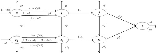
Figure 1.
Structure of Model (1).
Since the AIDS cases do not appear in other equations of (1), for dynamical analysis we only consider the subsystem
For stability analysis of the model (2), we obtain the fixed points of the system. Thus, we have to put . Therefore, the disease-free equilibrium point is obtained as
The endemic fixed point is , where
One can obtain as the answer of the non-linear algebraic system.
Definition 1.
The basic reproduction numberis the expected value of people in susceptible phase infected by an infective case [18,19].
means an infected individual produces on average less than one new infected person over its infectious period; therefore, the infection will not increase. Conversely, means each infected person causes more than one new infection on average. Thus, the disease will invade the population [19]. As mentioned in [16], by some calculation, for model (2), the education including basic reproduction number is obtained as
Theorem 1.
In model (2), if, then the disease-free fixed pointis locally asymptotically stable. If,is locally stable. If,is a saddle point with one eigenvalue having positive real part () and three eigenvalues having negative real part () [16].
2.2. Model without Education
If in model (2) we consider then, we obtain an HIV/AIDS epidemic model where education has no effect on the spread of infection. The model is as in the following ODE system [20]
Figure 2 explains the model structure.
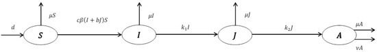
Figure 2.
Structure of Model (4).
As in the previous section, for stability analysis of the model, we consider the subsystem
The disease-free and endemic fixed points are and , respectively.
By some calculations, the reproduction number is obtained as
We can conclude that the relationship between the steady state of the system (5) and the corresponding reproduction number by the following theorem:
Corollary 1.
The disease-free fixed point of (5),, is locally asymptotically stable if , locally stable if, and is a saddle point if [20].
Corollary 2.
If, then, the positive fixed pointof the model (5) is locally asymptotically stable [20].
2.3. Impact of Education on HIV Transmission
To study the impact of public health education on preventing the growth of HIV/AIDS in society, we reconsider and as the basic reproduction number in the absence and presence of education, respectively, as
and
Therefore,
where
Notice that, due to , so , thus, by some calculations, we can conclude . Hence, is a factor to prevent the spread of HIV, which depends on educational parameters.
Now, public health education might be unnecessary if , because HIV/AIDS will not develop into an epidemic. Conversely, if , HIV will be epidemic, and the existence of education is undeniable. Therefore, we want to specify the necessary values for educational parameters to reduce the rate of development of HIV/AIDS.
3. Single and Multi-Objective Optimization
The optimization problem finds solution or solutions in a set of possible cases by observing the constraints of the problem with the conditions of optimizing the criteria for an optimization problem. The following problem is the optimization of a model to economize the expenses of education to obtain the best result in controlling the disease.
In general, it can be said that the data of the optimization problem is a function of variables or parameters of the model which is called cost function, the objective function (minimization) or utility function (maximization). The output of the optimization algorithm is defined as cost or profit.
A practical solution is called an optimal solution whenever it optimizes the objective function. In mathematics, common optimization problems are typically based on the minimization of cost functions.
Multi-objective optimization [21,22] deals with optimizing two or more conflicting objects simultaneously, which are dependent on a set of specific constraints. If the optimization of one objective results in the automatic optimization of the other one, it is not considered a multi-objective optimization problem.
In this paper, single and multi-objective optimization techniques are presented for optimizing the presented dynamic model (2).
3.1. Single Objective Optimization Problem
At first, we present the optimization problem as a single objective optimization problem according to the property of , and we focus on the Genetic Algorithm (GA) and Simulated Annealing (SA) optimization method to optimize the parameter , , and in a dynamic model (1). Our optimization strategy guarantees the as the main constraint. Hence, we keep as close as possible to , especially at the final time . Therefore, the optimization strategy will be finding the optimal values for parameters , , and such that the following nonlinear continuous time-cost function is minimized:
subject to the dynamic constraint (HIV/AIDS epidemic dynamic model (2)) and
where
Enumerative methods are the basis of the Guided Random Search (GRS) techniques, but they apply extra data about the study area to guide the search in the direction of the potential zone. SA technique that applies thermodynamic evolution to explore for the minimum-energy condition and evolutionary algorithms such as GA are good examples of GRS techniques.
The GRS methods, such as GA and SA, are beneficial in problems where the search area is huge, discontinuous, multi-modal, and where a near optimal solution is acceptable.
In this study, we use GA and SA methods to find the numerical solution of a presented optimal problem. To illustrate the stability analysis outlined in the previous section, we give some simulations using values of the parameters given in Table 2 [23]. We also obtain a reproduction number for these values of parameters. To obtain the phase diagrams, a fourth-order Runge-Kutta numerical code is applied using MATLAB software.
Table 2.
Explanation and values of parameter.
By considering the parameter values given in Table 2, simulation results are presented in Figure 3, Figure 4, Figure 5, Figure 6 and Figure 7.
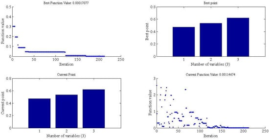
Figure 3.
Simulated Annealing (SA) optimization parameter of the model when c = 2.
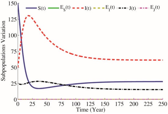
Figure 4.
Simulations of the model without education, when , and .
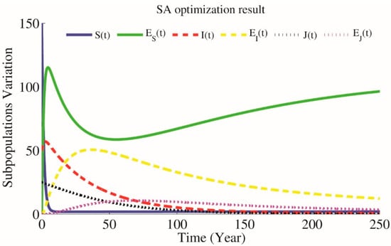
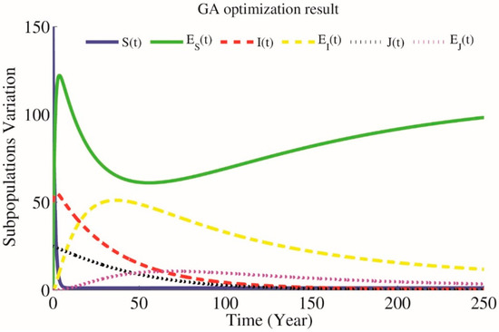
Figure 5.
Simulations of the model with public health education when , .
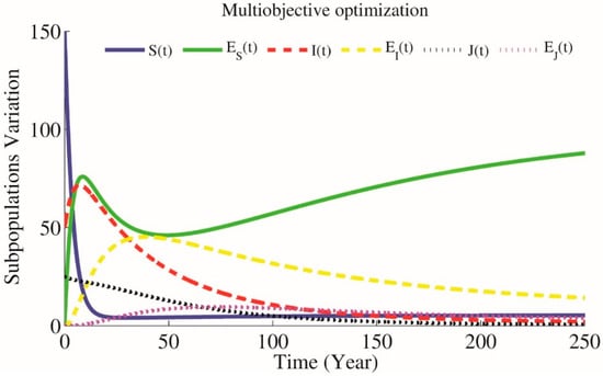
Figure 6.
Simulations of the model when parameters have been optimized by Genetic Algorithm (GA) multi optimization, , , , &
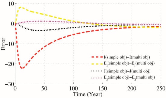
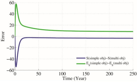
Figure 7.
Difference between GA simple and multi optimization results when , .
In SA simulation, when the average change is smaller than the function tolerance, the algorithm will stop. Also, note that the current schedule of the SA algorithm is not necessarily the optimal schedule explored until now. Thus, Figure 3 created a second plot that will show the optimal schedule explored until now. Figure 3 shows that the best point for parameters (, and ) is the final optimization point selected in the final schedule.
In Figure 4, we consider , and . It concludes that , which means that an infected individual over its infectious period produces on average new infected individuals. This means that when there is no public education to prevent HIV transmission, the disease will be developed into an epidemic state. As you can see in Figure 4, HIV-positive subpopulation is growing rapidly. In this situation, for reducing the spread of HIV infection, we obtain reasonable values of the parameter , and . According to the optimization problems (9)–(11), will be as close as possible to and by using SA technique for approximating the optimum of a given function (9) we will have parameters and as optimal parameters on which . Furthermore, by using the GA technique after generations we will have optimal parameters and as optimal parameters where . In Figure 5, we can see that by applying public health education and increasing educated individuals, the reproduction number equals , which is less than one, meaning that an infected individual produces on average new infected individual over its infectious period. Therefore, the HIV-positive subpopulation decreases and will approach zero in a long time, which means that the disease will be controlled in society. This shows that the education prevents susceptible people from HIV transmission.
Above: Simulations of the model when parameters have been optimized by SA optimization, , , , & . Bottom: Simulations of the model when parameters have been optimized by GA optimization, ,, , & .
3.2. Multi-Objective Optimization or Pareto Optimization Problem
In the next step, we replace the cost of single-objective optimization problems (9)–(11) with multi-objective cost function where the new optimization goal (cost) is to keep close to and as close as possible to , especially at the final time . Thus, our optimization problem can be formulated as follows:
where
subject to the dynamic constraint of HIV/AIDS epidemic dynamic model (2) and.
Our cost function consists of five objectives, each with three decision variables of , and . Also, bound constraint on the decision variables is imposed. Genetic algorithms are a kind of evolutionary algorithm, which are common instances of multiple-point search, in which random selection is applied as a tool to instruct an extremely explorative search via coding the parameter area. GA multi-objective optimization uses genetic algorithm to find a local Pareto front for multiple objective functions. In the following, we depend on multi-objective GA algorithm to find the numerical solution of the presented optimal problems (12)–(14).
Our multi-objective GA algorithm uses a variant of NSGA-II [21]. Fifty initial values are made randomly and the next production of the values is computed using the non-dominated rank and a distance measure of the amount in the current production. A non-dominated rank is specified to each amount using the relative compatibility. Also, the distance measure of an amount is used to compare amounts with equal rank. It is a measure of how far an amount is from the other amounts with the same rank.
According to the presented optimization problem that keeps close to and close to and using NSGA-II technique for approximating the optimum of a given function (12) we will have parameters , and as optimal parameters on which . Results are simulated in Figure 6. Also Figure 7 presents the difference between GA simple and multi optimization results.
4. Conclusions
We can understand from the above discussions that in an uneducated society, when , the spread of HIV/AIDS infection is unstoppable; therefore, the requirement of public health education is undeniable. In this condition, we should determine appropriate values for , , and . On the other hand, according to the dependence of education, reproduction number to , and , we can consider as to highlight the significant role of public health education in controlling HIV/AIDS. Since education about preventing HIV transmission is costly, we should consider optimizing the public health education parameters , and . We optimize these parameters by GA and SA. Note that, these values obtained in this paper are not unique, and some parameters might come forward, which are better or more applicable. We just explain a method to find suitable values for parameters of education. For future work, it is suggested to use stationary and cyclostationary time series models and regression analysis [24,25,26,27,28,29,30,31,32,33,34,35,36] to model and optimize the problem and compare their results to the those of the proposed technique in this work.
Author Contributions
M.H.O., S.B., and M.R.M. conceived and designed the experiments; M.H.O., S.B. carried out the experiments; M.R.M. analyzed the data; M.H.O., S.B. wrote the paper with aid of M.R.M. All authors have read and agreed to the published version of the manuscript.
Funding
This research received no external funding.
Conflicts of Interest
The authors declare no conflict of interest.
References
- Anderson, R.M. The role of mathematical models in the study of HIV transmission and the epidemiology of AIDS. J. Acq. Immun. Def. Synd. 1988, 1, 241–256. [Google Scholar]
- Anderson, R.M.; Medly, G.F.; May, R.M.; Johnson, A.M. A preliminary study of the transmission dynamics of the Human Immunodeficiency Virus (HIV), the causative agent of AIDS. Math. Med. Biol. 1986, 3, 229–263. [Google Scholar] [CrossRef] [PubMed]
- May, R.M.; Anderson, R.M. Transmission dynamics of HIV infection. Nature 1987, 326, 137–142. [Google Scholar] [CrossRef] [PubMed]
- Bachar, M.; Dorfmayr, A. HIV treatment models with time delay. C. R. Biol. 2004, 327, 983–994. [Google Scholar] [CrossRef]
- Blower, S. Calculating the consequences: HAART and risky sex. AIDS 2001, 15, 1309–1310. [Google Scholar] [CrossRef]
- Hethcote, H.W.; Van Ark, J.W. Modelling HIV Transmission and AIDS in the United States; Lectures Notes in Biomathematics; Springer: New York, NY, USA, 1992. [Google Scholar]
- Hsieh, Y.H.; Chen, C.H. Modelling the social dynamics of a sex industry: Its implications for spread of HIV/AIDS. Bull. Math. Biol. 2004, 66, 143–166. [Google Scholar] [CrossRef]
- Leenheer, P.D.; Smith, H.L. Virus dynamics: A global analysis. SIAM J. Appl. Math. 2003, 63, 1313–1327. [Google Scholar]
- McCluskey, C. A model of HIV/AIDS with staged progression and amelioration. Math. Biosci. 2003, 181, 1–16. [Google Scholar] [CrossRef]
- Perelson, A.S.; Nelson, P.W. Mathematical analysis of HIV-1 dynamics in vivo. SIAM Rev. 1999, 41, 3–44. [Google Scholar] [CrossRef]
- Samanta, G.P. Analysis of a nonautonomous HIV/AIDS epidemic model with distributed time delay. Math. Model. Anal. 2010, 15, 327–347. [Google Scholar] [CrossRef][Green Version]
- Samanta, G.P. Analysis of a nonautonomous HIV/AIDS model. Math. Model. Nat. Phenom. 2010, 5, 70–95. [Google Scholar] [CrossRef]
- Sharma, S.; Samanta, G.P. Dynamical Behaviour of an HIV/AIDS Epidemic Model. Differ. Equ. Dyn. Syst. 2014, 22, 369–395. [Google Scholar] [CrossRef]
- Wang, L.; Li, M.Y. Mathematical analysis of the global dynamics of a model for HIV infection of CD4^+ T-cells. Math. Biosci. 2006, 200, 44–57. [Google Scholar] [CrossRef] [PubMed]
- Wang, K.; Wang, W.; Liu, X. Viral infection model with periodic lytic immune response. Chaos Soliton Fractals 2006, 28, 90–99. [Google Scholar] [CrossRef]
- Ostadzad, M.H.; Shahmorad, S.; Erjaee, G.H. Dynamical analysis of public health education on HIV/AIDS transmission. Math. Methods Appl. Sci. 2014, 38, 3601–3614. [Google Scholar] [CrossRef]
- Ostadzad, M.H.; Shahmorad, S.; Erjaee, G.H. Study of public health education effect on spread of hiv infection in a density-dependent transmission model. Differ. Equ. Dyn. Syst. 2016. [Google Scholar] [CrossRef]
- Diekmann, O.; Heesterbeek, J.A.P.; Metz, J.A.J. On the definition and the computation of the basic reproduction ratio R_0 in models for infectious diseases in heterogeneous populations. J. Math. Biol. 1990, 28, 365–382. [Google Scholar] [CrossRef]
- Van Den Driessche, P.; Watmough, J. Reproduction numbers and sub-threshold endemic equilibria for compartmental models of disease transmission. Math. Biosci. 2002, 180, 29–48. [Google Scholar] [CrossRef]
- Cai, L.; Li, X.; Ghosh, M.; Guo, B. Stability analysis of an HIV/AIDS epidemic model with treatment. J. Comput. Appl. Math. 2009, 229, 313–323. [Google Scholar] [CrossRef]
- Deb, K. Multi-Objective Optimization Using Evolutionary Algorithms; John Wiley and Sons: Hoboken, NJ, USA, 2001. [Google Scholar]
- Del Valle, S.; Evangelista, A.M.; Velasco, M.C.; Kribs-Zaleta, C.M.; Hsu Schmitz, S.F. Effects of education, vaccination and treatment on HIV transmission in homosexuals with genetic heterogeneity. Math. Biosci. 2004, 187, 111–133. [Google Scholar] [CrossRef][Green Version]
- Mukandavire, Z.; Garira, W.; Tchuenche, J.M. Modelling effects of public health educational campaigns on HIV/AIDS transmission dynamics. Appl. Math. Model. 2009, 33, 2084–2095. [Google Scholar] [CrossRef]
- World Health Organization. UNAIDS Report on the Global AIDS Epidemic. 2004. Available online: http://unaids.org (accessed on 7 February 2020).
- Mahmoudi, M.R.; Nematollahi, A.R.; Soltani, A.R. On the detection and estimation of the simple harmonizable processes. Iran. J. Sci. Technol. A (Sci.) 2015, 39, 239–242. [Google Scholar]
- Mahmoudi, M.R.; Maleki, M. A new method to detect periodically correlated structure. Comput. Stat. 2017, 32, 1569–1581. [Google Scholar] [CrossRef]
- Nematollahi, A.R.; Soltani, A.R.; Mahmoudi, M.R. Periodically correlated modeling by means of the periodograms asymptotic distributions. Stat. Pap. 2017, 58, 1267–1278. [Google Scholar] [CrossRef]
- Mahmoudi, M.R.; Heydari, M.H.; Avazzadeh, Z.; Pho, K.H. Goodness of fit test for almost cyclostationary processes. Digit. Signal Process 2020, 96, 102597. [Google Scholar] [CrossRef]
- Mahmoudi, M.R.; Heydari, M.H.; Roohi, R. A new method to compare the spectral densities of two independent periodically correlated time series. Math. Comput. Simulat. 2019, 160, 103–110. [Google Scholar] [CrossRef]
- Mahmoudi, M.R.; Heydari, M.H.; Avazzadeh, Z. Testing the difference between spectral densities of two independent periodically correlated (cyclostationary) time series models. Commun. Stat. Theory Methods 2019, 48, 2320–2328. [Google Scholar] [CrossRef]
- Mahmoudi, M.R.; Maleki, M.; Pak, A. Testing the Difference between Two Independent Time Series Models. Iran. J. Sci. Technol. A (Sci.) 2017, 41, 665–669. [Google Scholar] [CrossRef]
- Mahmoudi, M.R.; Heydari, M.H.; Avazzadeh, Z. On the asymptotic distribution for the periodograms of almost periodically correlated (cyclostationary) processes. Digit. Signal Process 2018, 81, 186–197. [Google Scholar] [CrossRef]
- Mahmoudi, M.R.; Mahmoodi, M. Inferrence on the Ratio of Correlations of Two Independent Populations. J. Math. Ext. 2014, 7, 71–82. [Google Scholar]
- Mahmoudi, M.R.; Mahmoudi, M.; Nahavandi, E. Testing the Difference between Two Independent Regression Models. Commun. Stat. Theory Methods 2016, 45, 6284–6289. [Google Scholar] [CrossRef]
- Mahmoudi, M.R.; Maleki, M.; Pak, A. Testing the Equality of Two Independent Regression Models. Commun. Stat. Theory Methods 2018, 47, 2919–2926. [Google Scholar] [CrossRef]
- Mahmoudi, M.R. On Comparing Two Dependent Linear and Nonlinear Regression Models. J. Test. Eval. 2018, 47, 449–458. [Google Scholar] [CrossRef]
© 2020 by the authors. Licensee MDPI, Basel, Switzerland. This article is an open access article distributed under the terms and conditions of the Creative Commons Attribution (CC BY) license (http://creativecommons.org/licenses/by/4.0/).