A Heuristic Simulation–Optimization Approach to Information Sharing in Supply Chains

Abstract

The sustainability of the supply chain is possible only if the profitability of all the tiers participating in that supply chain is guaranteed. The profitability of each of these tiers is ensured if information sharing as well as an effective and seamless coordination system are realized between the tiers. This process reduces the influence of an important risk factor known as the bullwhip effect. The purpose of the current study is to determine the necessary information sharing level to optimize the supply chain that has asymmetric flows of input and output values and to examine the effects of information sharing on the order fill rate (OFR) and total inventory cost (TIC) of the supply chain through analysis of variance (ANOVA) testing. In this work, the supply chain was optimized by using the particle swarm optimization (PSO) technique, with an objective function that assumes the maximization of OFR and minimization of TIC. The proposed method showed excellent results in comparing the mean, variance, and coefficient of variation. In addition, the method used the ANOVA test with a 5% significance level to verify the impact of the information sharing level.

1. Introduction

Supply chain management (SCM) is defined as a way to maximize profitability while keeping the overall cost of the supply chain to a minimum and meeting the customer’s service requirements at the same time. SCM is described as a systematic method that can be used to effectively integrate suppliers, manufacturers, distributors, and retailers so that an optimal product can be delivered in optimal amounts, at an optimal location, and at the optimal time [1]. The most ideal supply chain is the symmetric chain in which the product quantity, equal to the order quantity of the tier, is transferred from the upstream tier to the downstream tier. However, information sharing is not enabled and shows asymmetric results that differ between input and output values. Supply chains are complicated systems, involving, for example, demand handling, lead-times, batch orders, payments, price changes, and promotions [2]. This means that unexpected problems can arise. The most prominent of these is the “bullwhip effect”, whereby errors in demand forecasts increase along the supply chain [3].

Typically, the bullwhip effect is influenced by the level of information sharing [4,5], lead time [6], forecasting method [7], and inventory policy [8]. Lee and Wu [8] showed that inventory management is significant in supply chain management, and efficient inventory management can improve customer satisfaction, balance product plans, and reduce operating costs. In another study, Graves [7] investigated the effect of forecasting methods on the bullwhip effect. Furthermore, Chen et al. [6] used a simulation to validate the idea that an increase in the bullwhip effect is directly associated with lead time, and explained that the lead time has an effect on the safety of the inventory level and demand forecasting. Lee and Whang [5] demonstrated that information sharing has a significant effect on the determination of order quantity for a supplier in terms of reducing the inventory level and cost.

One of the methods to resolve the bullwhip effect is to allow each tier such as the supplier, manufacturer, distributor, and retailer to share information [9,10]. However, Chatfield et al. [9] indicated that this may increase the bullwhip effect as the range of order fluctuation becomes wider if a tier completely trusts order information. Their research indicated that information sharing can be effective only if the downstream information has a certain level of reliability; however, the level of information sharing was not considered by the authors.

Earlier studies concentrated on the effects of information sharing, inventory policy, and forecasting policy on the bullwhip effect, rather than the reduction of the total inventory cost (TIC) or the enhancement of the order fill rate (OFR) by improving the performance of the entire supply chain [11,12]. A supply chain that is sustainable and robust should be able to address all the problems that arise from the supply chain, as described by the bullwhip effect, and achieve supply chain optimization from a global perspective to ensure that all tiers participating in the supply chain are profitable.

One of the most effective ways to increase the sustainability of a supply chain to accomplish overall optimization is to reduce uncertainty in the supply chain and strengthen the partnership with the tiers participating in the supply chain by allowing the maximum information sharing among those tiers. To this end, the current study analyzes the level of information sharing and its effect on the supply chain by varying the level. The particle swarm optimization (PSO) technique has been used to optimize the overall supply chain, and the objective assumes the minimization of TIC and maximization of OFR. The effect of θ, which is the level of information sharing, was verified via ANOVA.

In this paper, therefore, first, the level of information sharing (θ) that optimizes the TIC and OFR, which are the objectives of the supply chain, was determined using PSO. Second, this result was compared with the condition when the level of information sharing is different. Third, ANOVA was used to evaluate the impact between information sharing levels and significant impact on TIC and OFR.

The rest of this paper is organized as follows. Section 2 provides a literature review, and the characteristics of the proposed model are shown in Section 3. The simulation of the model and analysis of the results are presented in Section 4, and a discussion is presented in Section 5. Finally, the suggested method is formalized and future work is discussed in Section 6.

2. Literature Review

The problem considered in this study can be classified as a simulation–optimization problem in which the supply chain model used in the experiment was implemented as a simulation model and the result was obtained through the optimization process. In addition, the supply chain model used in this study was classified as a discrete stochastic simulation–optimization model that targets discrete decision variables rather than continuous decision variables.

The discrete stochastic simulation–optimization techniques with discrete decision variables include learning automata [13], ranking-and-selection [14], simulated annealing [15], stochastic comparison method [16], evolutionary algorithm [17], etc.

Among these methods, the meta-heuristic method that can be applied regardless of the type of problem or the size of decision variables are evolutionary algorithms, of which the genetic algorithm and PSO technique are representatives [18]. This study applies the PSO technique because it uses primitive and simple mathematical operators, is very efficient in terms of the memory requirements and execution speed of the computer, and is much more efficient than the genetic algorithm in certain specific areas [19,20]. The PSO is an efficient algorithm for feature selection areas because the method is faster to converge and easier to implement when compared to other meta heuristic algorithms [21]. Additionally, the PSO is one of the most important meta heuristic algorithms in the field of collective intelligence [22]. A detailed description of the PSO technique is described in detail in Section 3.

Members of the supply chain have a different range of information that needs to be shared, and sharing information is necessary to make good decisions, increase visibility among members, and increase profitability, but the risk of information leakage affects a company’s competitive advantage [23]. An important prerequisite for information sharing is supply chain integration (SCI), which is important in the information sharing process because SCI enhances the connectivity, coordination, and collaboration between members of the supply chain. Therefore, information sharing with customers, information sharing with suppliers, information sharing with functions, and information sharing with the organization should all be included [24]. Information sharing and technology are some of the main factors in coordination between parties in a supply chain. In particular, information sharing improves the efficiency of the supply chain because information sharing reduces the inventory and facilitates production, thereby increasing supply chain efficiency [25]. Information sharing provides the manufacturing sector with benefits such as reduced inventory and efficient inventory management, reduced costs, increased visibility (significantly reduced uncertainty), significantly reduced or eliminated bullwhip effects, improved resource utilization, improved productivity, improved organizational efficiency, improved service, social bond building and strengthening, early problem detection, rapid response, reduced time from ordering to delivery, and optimized capacity. However, there are also difficulties in implementing information sharing [26].

The studies presented above emphasized the importance of information sharing, but did not provide an optimization perspective that would make information sharing more efficient. Therefore, this study aims to provide the most desirable level of information sharing for participants in the supply chain by considering information sharing and non-sharing while applying the simulation–optimization approach.

3. The Proposed Model

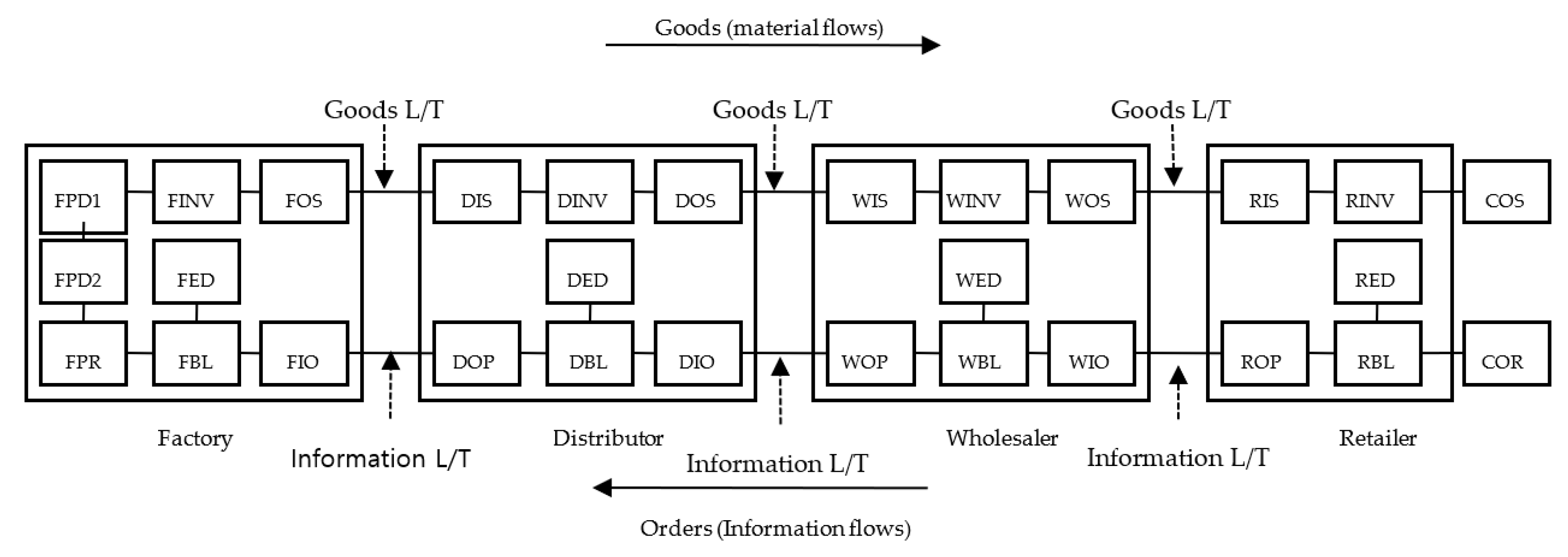
The supply chain we studied comprised a factory, distributor, wholesaler, and retailer, as depicted in Figure 1.

The decision variables used in this study (Figure 1) are illustrated as follows:

$\mathrm{FPD}{1}_{\mathrm{t}}$: the production delay 1 of a factory at time t

$\mathrm{FPD}{2}_{\mathrm{t}}$: the production delay 2 of a factory at time t

${\mathrm{FED}}_{\mathrm{t}}$: the expected demand of a factory at time t

${\mathrm{FOS}}_{\mathrm{t}}$: the outgoing shipment of a factory at time t

${\mathrm{FIO}}_{\mathrm{t}}$: the incoming order of a factory at time t

${\mathrm{FPR}}_{\mathrm{t}}$: the production of a factory at time t

${\mathrm{FBL}}_{\mathrm{t}}$: the backlog of a factory at time t

${\mathrm{FINV}}_{\mathrm{t}}$: the inventory of a factory at time t

${\mathrm{DED}}_{\mathrm{t}}$: the expected demand of a distributor at time t

${\mathrm{DOS}}_{\mathrm{t}}$: the outgoing shipment of a distributor at time t

${\mathrm{DIO}}_{\mathrm{t}}$: the incoming order of a distributor at time t

${\mathrm{DIS}}_{\mathrm{t}}$: the incoming shipment of a distributor at time t

${\mathrm{DOP}}_{\mathrm{t}}$: the order placed by a distributor at time t

${\mathrm{DBL}}_{\mathrm{t}}$: the backlog of a distributor at time t

${\mathrm{DINV}}_{\mathrm{t}}$: the inventory of a distributor at time t

${\mathrm{WED}}_{\mathrm{t}}$: the expected demand of a wholesaler at time t

${\mathrm{WOS}}_{\mathrm{t}}$: the outgoing shipment of a wholesaler at time t

${\mathrm{WIO}}_{\mathrm{t}}$: the incoming order of a wholesaler at time t

${\mathrm{WIS}}_{\mathrm{t}}$: the incoming shipment of a wholesaler at time t

${\mathrm{WOP}}_{\mathrm{t}}$: the order placed by a wholesaler at time t

${\mathrm{WBL}}_{\mathrm{t}}$: the backlog of a wholesaler at time t

${\mathrm{WINV}}_{\mathrm{t}}$: the inventory of a wholesaler at time t

${\mathrm{RED}}_{\mathrm{t}}$: the expected demand of a retailer at time t

${\mathrm{ROS}}_{\mathrm{t}}$: the outgoing shipment of a retailer at time t

${\mathrm{RIO}}_{\mathrm{t}}$: the incoming order of a retailer at time t

${\mathrm{RIS}}_{\mathrm{t}}$: the incoming shipment of a retailer at time t

${\mathrm{ROP}}_{\mathrm{t}}$: the order placed by a retailer at time t

${\mathrm{RBL}}_{\mathrm{t}}$: the backlog of a retailer at time t

${\mathrm{RINV}}_{\mathrm{t}}$: the inventory of a retailer at time t

${\mathrm{COR}}_{\mathrm{t}}$: the order of a customer at time t

In the supply chain (Figure 1), the factory receives orders from the distributor, the distributor from the wholesaler, the wholesaler from the retailer, and the retailer from the customers. In this sequence, an upstream tier interprets the information related to the order quantity received from a downstream tier. If there is no information sharing between the tiers, the upstream tier is severely affected by the bullwhip effect and experiences a much greater demand distortion and variance amplification than the downstream tier. On the other hand, if the upstream tier receives sufficient information from the downstream tier, the reliability of the received order is high. In such a case, when new expected demand (${\mathrm{ED}}_{\mathrm{t}}$) is determined, a large weight is put on the incoming order (${\mathrm{IO}}_{\mathrm{t}-1}$) which is the order placed (${\mathrm{OP}}_{\mathrm{t}-1}$) by the downstream tier, and less weight is put on past expected demand (${\mathrm{ED}}_{\mathrm{t}-1}$). In the present study, to evaluate the level of information sharing, Equation (1) is used for ${\mathrm{ED}}_{\mathrm{t}}$, ${\mathrm{ED}}_{\mathrm{t}-1}$, and ${\mathrm{IO}}_{\mathrm{t}-1}$ by the proper adjustment of their weight.

$${\mathrm{ED}}_{\mathrm{t}}=\mathsf{\theta }·{\mathrm{ED}}_{\mathrm{t}-1}+\left(1-\mathsf{\theta }\right)·{\mathrm{IO}}_{\mathrm{t}-1}$$

(1)

where ${\mathrm{ED}}_{\mathrm{t}}$ and ${\mathrm{ED}}_{\mathrm{t}-1}$ are the expected demand at time t and t − 1, respectively; ${\mathrm{IO}}_{\mathrm{t}-1}$ is the actual demand ordered at time t − 1; and $\mathsf{\theta }$ ($0\le \mathsf{\theta }\le 1$) is the relative weight between the expected demand and the actual demand. That is, expected demand (${\mathrm{ED}}_{\mathrm{t}}$) means the sum of the incoming order (${\mathrm{IO}}_{\mathrm{t}-1}$) from the downstream tier to the additional expected demand (${\mathrm{ED}}_{\mathrm{t}-1}$) determined through its own information to prevent a shortage due to uncertainties in information coming from the downstream tier. When θ = 0, there is 100% confidence in the information of the order (${\mathrm{IO}}_{\mathrm{t}-1}$) originating from the downstream tier. If θ = 1, the information coming from the downstream tier cannot be trusted, implying that ${\mathrm{ED}}_{\mathrm{t}}$ is self-determining, and there is no need for any shared information. Thus, the closer value θ is to 0, the higher the level of information sharing.

Equation (1) can be transformed to Equation (2) if the quantity ordered by the customer is disclosed at each tier. In Equation (2), ${\mathrm{COR}}_{\mathrm{t}-1}$ denotes the order quantity of the customer at time t − 1. If the upstream tier has sufficient information sharing with the downstream tier, it can reduce the dependence on the expected demand (${\mathrm{ED}}_{\mathrm{t}-1}$) because it can accurately identify and trust the attributes of the order (${\mathrm{COR}}_{\mathrm{t}-1}$) from the customer.

$${\mathrm{ED}}_{\mathrm{t}}=\mathsf{\theta }·{\mathrm{ED}}_{\mathrm{t}-1}+\left(1-\mathsf{\theta }\right)·{\mathrm{COR}}_{\mathrm{t}-1}$$

(2)

Since the supply chain involves many tiers and is exposed to various situations and problems, a value of θ close to 0 does not indicate that the entire supply chain is optimal. That is, θ, which satisfies the total tiers involved in the supply chain, may have a value other than zero. Therefore, to analyze the influence of information sharing in supply chains, the value of θ should be varied. This is because the satisfaction of a supply chain varies with changes in the θ-value, which signifies changes in the level of information sharing. As the tiers involved in the supply chain are all different and the levels of information are different, the θ value that satisfies the entire supply chain should be determined as appropriate for the supply chain situation, not θ = 0, as the ideal level of information sharing that reflects 100% of customer demand.

In this study, optimization is achieved by applying PSO, a meta-heuristic method based on the social behavior of biological groups such as a flock of birds or a school of fish, rather than a genetic algorithm, to imitate the natural evolutionary process [30]. The PSO method regards a decision variable as a particle, and the population of decision variables is considered as a swarm. It is important to note that the PSO algorithm finds the optimal solution by moving particles, and the movement of the particles are updated via the position equation, Equation (3), and the velocity equation, Equation (4).

$$\mathrm{Position}:{\mathrm{X}}_{\mathrm{nk}}^{\left(\mathrm{t}+1\right)}={\mathrm{X}}_{\mathrm{nk}}^{\left(\mathrm{t}\right)}+{\mathsf{\chi }\mathrm{V}}_{\mathrm{nk}}^{\left(\mathrm{t}\right)}+{\mathsf{ϵ}}^{\left(\mathrm{t}\right)}$$

(3)

$$\mathrm{Velocity}:{\mathrm{V}}_{\mathrm{nk}}^{\left(\mathrm{t}+1\right)}={\mathrm{wV}}_{\mathrm{nk}}^{\left(\mathrm{t}\right)}+{\mathrm{c}}_1{\mathrm{r}}_1\left({\mathrm{P}}_{\mathrm{nk}}-{\mathrm{X}}_{\mathrm{nk}}^{\left(\mathrm{t}\right)}\right)+{\mathrm{c}}_2{\mathrm{r}}_2\left({\mathrm{G}}_{\mathrm{nk}}-{\mathrm{X}}_{\mathrm{nk}}^{\left(\mathrm{t}\right)}\right)$$

(4)

The velocity of each particle, ${\mathrm{v}}_{\mathrm{nk}}^{\left(\mathrm{t}+1\right)}$, is updated considering both the particle optimum, ${\mathrm{P}}_{\mathrm{nk}}$, and the global optimum, ${\mathrm{G}}_{\mathrm{nk}}$. ${\mathrm{v}}_{\mathrm{nk}}^{\left(\mathrm{t}+1\right)}$ is the velocity of the kth component of the nth particle of the t + 1th generation.${\mathrm{P}}_{\mathrm{nk}}$ is the particle optimum that is found by each particle up to the present time, and ${\mathrm{G}}_{\mathrm{nk}}$ is the global optimum that is found by population to share information and search the place. ${\mathrm{r}}_1$ and ${\mathrm{r}}_2$ are random variables uniformly distributed on the interval [0, 1], and ${\mathrm{c}}_1$ and ${\mathrm{c}}_2$ are acceleration constants adjusting the effect of the particle optimum and the effect of the group optimum [12]. $\mathrm{w}$ is the inertia weight and limits this velocity.

Furthermore, the PSO prevents algorithms from converging to local optima by using the position, velocity, inertia weight, acceleration constants, and population size. The PSO, one of meta heuristic methods, is used as an optimization methodology in order to allow for the information sharing level. The method uses primitive and simple mathematical operators and is known to be highly efficient in memory requirement and running speed [18,19]. In addition, it shows superiority to genetic algorithm (GA) in some application areas [20]. The PSO is considered to be simpler and more efficient than a genetic algorithm [12,18].

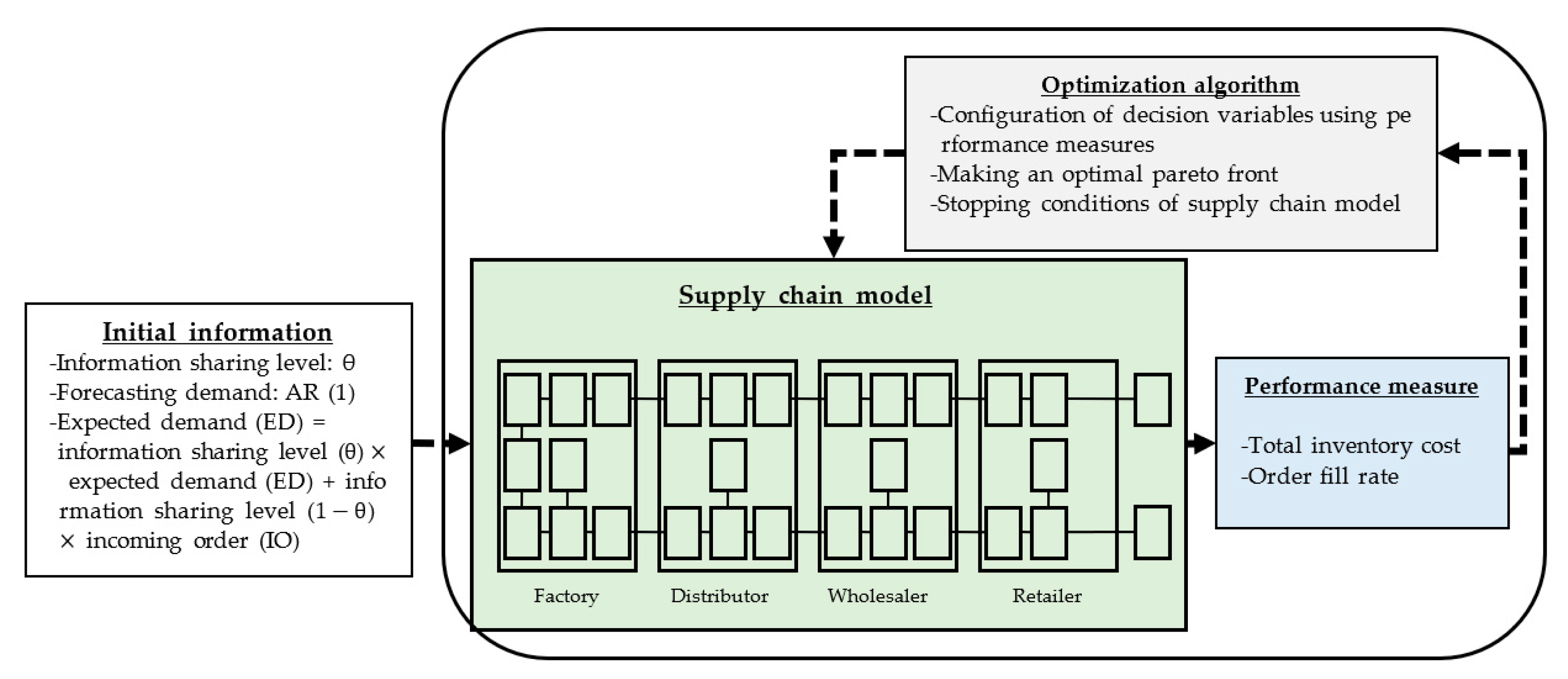
Our proposed model is graphically explained in Figure 2. The initial information for supply chain optimization is the information sharing level (θ), AR (1), which represents customer demand, and the expected demand reflecting the level of information sharing. The supply chain model accepts the initial information, performs the simulation, and confirms the values of TIC and OFR. The optimization process is performed using PSO as the optimization method. If the optimization condition of the supply chain model is satisfactory, the model execution is terminated. Otherwise, the model is executed until a satisfactory optimization condition is realized.

4. Experiment and Results Analysis

A demand from the end-customer was assumed to be stochastic and to follow a first-order autoregressive process (AR (1)) via the following expression:

$${\mathrm{D}}_{\mathrm{t}}=\mathsf{\mu }+{\mathsf{\rho }\mathrm{D}}_{\mathrm{t}-1}+{\mathsf{ϵ}}_{\mathrm{t}},\mathrm{where}\left|\mathsf{\rho }\right|<1$$

(5)

Furthermore, ${\mathrm{D}}_{\mathrm{t}}$ is the end-customer demand at time t; $\mathsf{\mu }$ is a non-negative constant; ${\mathsf{ϵ}}_{\mathrm{t}}$ is the error term following independent and identical distribution (i.i.d.) with a mean of 0 and a standard deviation ${\mathsf{\sigma }}^2$; and $\mathsf{\rho }$ is the first-order autocorrelation coefficient.

The expected demand for each tier was estimated by adding the actual order from the downstream to the expected demand of the current tier using Equation (1). Now, the smaller the $\mathsf{\theta }$ value, the higher the importance of the actual demand from downstream and the smaller the weight of the expected demand including uncertainty. If the end-customer demand is shared through the supply chain, the expected demand is calculated using Equation (2). The TIC for a supply chain is estimated by the following expression:

$${{\displaystyle \sum }}_{\mathrm{t}=1}^{\mathrm{n}}\left(\mathrm{BLC}\left({{\displaystyle \sum }}_{\mathrm{i}=1}^{\mathrm{m}}{\mathrm{BL}}_{\mathrm{t},\mathrm{i}}\right)+\mathrm{HIC}\left({{\displaystyle \sum }}_{\mathrm{i}=1}^{\mathrm{m}}{\mathrm{INV}}_{\mathrm{t},\mathrm{i}}\right)\right).$$

(6)

The TIC consists of the sum of the shortage cost (BLC) and inventory holding cost (HIC) at each tier (i = 1, …, m) during time t (t = 1, …, n). The shortage cost is assumed to be higher than the inventory holding cost, because a shortage causes a tier to forego a sales opportunity as well as the reliability of the tier. ${\mathrm{BL}}_{\mathrm{t},\mathrm{i}}$ is the amount of shortage and ${\mathrm{INV}}_{\mathrm{t},\mathrm{i}}$ is the amount of inventory in tier i at time t.

Typical inventory replenishment policies are implemented: order-up-to level policy, an order point-order quantity (s, Q) system, order point-order up to level (s, S) system, periodic review order up to level (R, S) system, and an (R, s, S) system [31]. In the (s, Q) system, a fixed Quantity Q is ordered whenever the inventory position drops to the reorder point s or lower. S means s + Q and R means every R units of time. We determined the optimal order quantity by using ${\mathrm{OP}}_{\mathrm{t},\mathrm{i}}=\max \left\{0,{\mathrm{OP}}_{\mathrm{t},\mathrm{i}}^{\ast }\right\}$ in tier i at time t considering the inventory adjustments for each tier and for the entire supply chain, and ${\mathrm{OP}}_{\mathrm{t}}^{\ast }$ is represented by Equation (7) [28]:

$${\mathrm{OP}}_{\mathrm{t},\mathrm{i}}^{\ast }={\mathrm{ED}}_{\mathrm{t},\mathrm{i}}+{\mathrm{AS}}_{\mathrm{t},\mathrm{i}}+{\mathrm{ASL}}_{\mathrm{t},\mathrm{i}}$$

(7)

where ${\mathrm{ED}}_{\mathrm{t},\mathrm{i}}$ is the expected demand for each tier i at time t, and ${\mathrm{AS}}_{\mathrm{t},\mathrm{i}}$ is the inventory adjustment for each tier i at time t, as shown in Equation (8). ${\mathrm{ASL}}_{\mathrm{t},\mathrm{i}}$ is the inventory adjustment for the whole supply chain at time t and is calculated by summing the inventory adjustment for each tier i at time t, as shown in Equation (9):

$${\mathrm{AS}}_{\mathrm{t},\mathrm{i}}={\mathsf{\alpha }}_{\mathrm{S}}\left({\mathrm{DINV}}_{\mathrm{t},\mathrm{i}}-{\mathrm{INV}}_{\mathrm{t},\mathrm{i}}+{\mathrm{BL}}_{\mathrm{t},\mathrm{i}}\right)$$

(8)

where ${\mathrm{DINV}}_{\mathrm{t},\mathrm{i}}$ is the ideal inventory quantity for each tier i at time t; ${\mathrm{INV}}_{\mathrm{t},\mathrm{i}}$ is the actual current inventory level for each tier i at time t; and ${\mathrm{BL}}_{\mathrm{t},\mathrm{i}}$ is the shortage quantity for each tier i at time t. Furthermore, ${\mathsf{\alpha }}_{\mathrm{S}}$ is the ratio of discordance between the ideal inventory and the actual inventory in each round.

$${\mathrm{ASL}}_{\mathrm{t},\mathrm{i}}={\mathsf{\alpha }}_{\mathrm{SL}}\left(\mathrm{DSL}-{\mathrm{SL}}_{\mathrm{t},\mathrm{i}}\right)$$

(9)

where DSL is the ideal inventory quantity for the entire supply chain; ${\mathrm{SL}}_{\mathrm{t},\mathrm{i}}$ is the actual current inventory for each tier i in the supply chain; and ${\mathsf{\alpha }}_{\mathrm{SL}}$ is the ratio of the ideal inventory quantity to the actual current inventory quantity in each round. Using Equations (8) and (9), Strozzi et al. [28] defined order quantity (Q) as follows:

$$\mathrm{Q}={\mathrm{DINV}}_{\mathrm{t},\mathrm{i}}+\mathsf{\beta }·\mathrm{DSL},\mathrm{where}\mathsf{\beta }={\mathsf{\alpha }}_{\mathrm{SL}}/{\mathsf{\alpha }}_{\mathrm{S}},{\mathsf{\alpha }}_{\mathrm{SL}}<{\mathsf{\alpha }}_{\mathrm{S}},\left(\frac{{\mathsf{\alpha }}_{\mathrm{SL}}}{{\mathsf{\alpha }}_{\mathrm{S}}}\right)\le 1.$$

(10)

In Equation (10), high values of ${\mathsf{\alpha }}_{\mathrm{SL}}$ explain the high attention to the inventory, and high $\mathsf{\beta }$ values mean high attention to the supply chain in comparison with the inventory.

In the optimization algorithm, the input data include the level of initial information sharing, the forecasted demand for each tier, and expected demand. The optimization model consists of the supply chain model and the optimization algorithm (Figure 2). The supply chain model fetches initial information, performs the simulation, and sends the optimization algorithm and simulation result. Subsequently, the optimization algorithm performs PSO and builds a population by selecting the decision variables, the relative weight of the expected demand information of $\mathsf{\theta }$, and other additional parameters. The population obtained from the optimization algorithm becomes the optimal Pareto candidate set to satisfy the objectives.

The population is composed of the initial inventory level, the relative weight of the expected demand information of $\mathsf{\theta }$, shortage cost, and inventory holding cost, all of which were added at each tier in the supply chain. The population of parameters and decision variables generated a set of Pareto candidates during the optimization process. The decision variables and parameters were automatically adjusted according to the objective function. The optimization process iteratively performed the computation based on the model in Figure 2, minimized the TIC, and maximized the OFR by considering the information sharing level and other parameters.

The assumptions used for this simulation of the supply chain model are as follows [28]:

①

The lead time for the distributor, wholesaler, and retailer is one week;

②

The lead time for the factory tier is three weeks, considering the lead time of the raw-material supplier;

③

The capacity of each tier is infinite;

④

The order requested is never canceled; and

⑤

The inventory left is never returned.

Since it is difficult to obtain a theoretical value for a dynamic supply chain, we applied the same parameter values used by Strozzi et al. [28]. Thus, the customer demand model is AR(1) with $\mathsf{\rho }$= −0.6, $\mathsf{\mu }$= 100, and ${\mathsf{ϵ}}_{\mathrm{t}}$ follows a normal distribution, N(0, 10²). The range of $\mathsf{\theta }$ is between 0 and 1. The size of the population is 200, and the number of generations is 100. The information lead time and the material lead time are one week, and the total replication length and warm-up period are 600 weeks and 100 weeks, respectively. Since $\mathrm{Q}=17$, ${\mathsf{\alpha }}_{\mathrm{S}}=0.317$, and $\left(\frac{{\mathsf{\alpha }}_{\mathrm{SL}}}{{\mathsf{\alpha }}_{\mathrm{S}}}\right)=0.317$, as suggested by Strozzi et al. [28], are reasonable, we applied those values in the present work. The shortage and inventory holding costs were kept unchanged so that the simulation results could be compared objectively. The inventory holding cost was 0.5 per unit, and the shortage cost was 2 per unit per period.

The roles of the objective functions are to minimize the total inventory holding cost and maximize the OFR, as shown in Equations (11) and (12).

$$\mathrm{Minimize}\mathrm{TIC}={{\displaystyle \sum }}_{\mathrm{t}=1}^{\mathrm{n}}\left(\mathrm{BLC}\left({{\displaystyle \sum }}_{\mathrm{i}=1}^{\mathrm{m}}{\mathrm{BL}}_{\mathrm{t},\mathrm{i}}\right)+\mathrm{HIC}\left({{\displaystyle \sum }}_{\mathrm{i}=1}^{\mathrm{m}}{\mathrm{INV}}_{\mathrm{t},\mathrm{i}}\right)\right)$$

(11)

$$\mathrm{Maximize}\mathrm{OFR}={{\displaystyle \sum }}_{\mathrm{i}=1}^{\mathrm{m}}{\mathrm{OFR}}_{\mathrm{i}}/\mathrm{m}$$

(12)

In Equations (11) and (12), m is the number of tiers, and the overall OFR in the entire supply chain is represented by dividing the sum of the order fill rate (${\mathrm{OFR}}_{\mathrm{i}}$) for each tier by the number of tiers (m). Note that the objective of the OFR is to maximize Equation (6) of the end-customer’s OFR instead of the overall OFR. The OFR means the percentage of the number of orders that are satisfied among the final customer’s orders during the entire simulation time. The TIC is determined by the sum of BLC and HIC at all tiers during the entire simulation time, and OFR is calculated as the average of order satisfaction at all tiers during the entire simulation time.

The simulation was tested in two ways: (1) using Equation (1) based on the information from downstream, and (2) using Equation (2) based on the information from the end-customer. For both cases, two scenarios were compared: (1) when the relative weight of the expected demand information of $\mathsf{\theta }$ is automatically adjusted from 0 to 1, and (2) when the relative importance of the expected demand information of $\mathsf{\theta }$ is fixed to 0.25, as suggested by Strozzi et al. [28]. The difference between the two cases in that the end-customer information is used in the second case, and the relative weight of the expected demand information of $\mathsf{\theta }$ is fixed to 0.

4.1. The Case of Using the Downstream Information

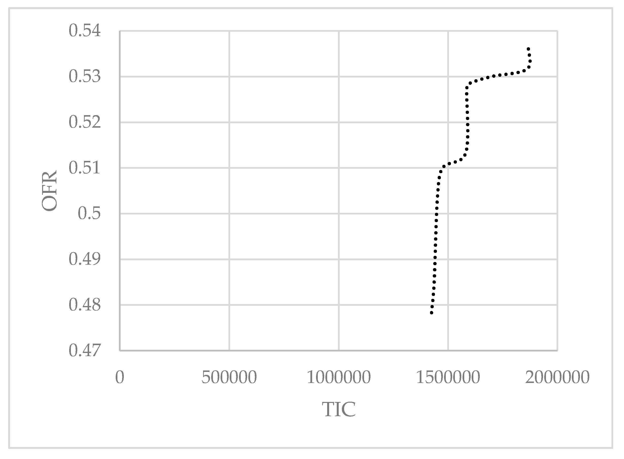
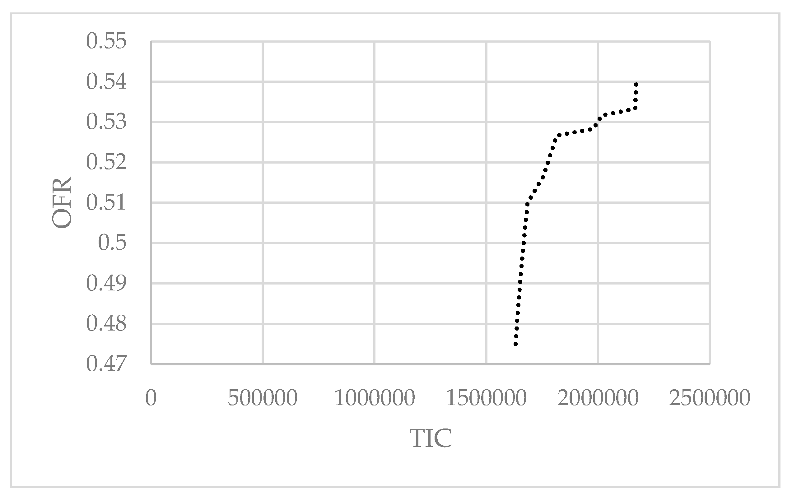
The simulation results for the first case are presented in Figure 3 and Figure 4, and the specific values are summarized in

Table 1. Total ranges of the inventory cost and order fill rate under non-information sharing conditions.

	$\mathsf{\theta }$	$\mathsf{\theta }\le 1$	$\mathsf{\theta }=0.25$
Objectives
Total inventory cost	Min	1,424,416.167	1,630,458.682
	Max	1,866,388.589	2,170,367.994
Order fill rate	Min	0.478	0.475
	Max	0.537	0.540

.

As shown in Table 1, the TIC, by adjusting $\mathsf{\theta }$ from 0 to 1, was between 1,424,416.167 and 1,866,388.589, and the TIC, when $\mathsf{\theta }$ was set to 0.25, was between 1,630,458.682 and 2,170,367.994. The range of OFR, when $\mathsf{\theta }$ has a constant value of 0.25, was 0.475 to 0.54, and the range of the OFR, by adjusting $\mathsf{\theta }$ from 0 to 1, was 0.478 to 0.537.

A detailed comparison of TIC was carried out by summarizing the statistical total inventory cost data for both scenarios (see

Table 2. Statistical analysis of total inventory cost under non-information sharing conditions.

Factor	N	Total	Mean	Variance
TIC(0 $\le$ θ $\le$ 1)	200	324,948,399.5	1,624,741.998	25,534,935,240
TIC(θ = 0.25)	200	378,125,334.5	1,890,626.672	39,302,200,428

).

As shown in Table 2, both the mean and variance of TIC were lower when θ was automatically adjusted, and it seems that adjusting $\mathsf{\theta }$ from 0 to 1 is a more effective solution than fixing $\mathsf{\theta }$ to 0.25 in terms of TIC. This was validated further by performing an ANOVA test at the 0.05 level of significance to determine whether any significant difference in the TIC between the two scenarios could be found. The result of the ANOVA test is summarized in

Table 3. ANOVA test result for total inventory cost under non-information sharing conditions.

Cause of Variance	Sum of Squares	df	Mean Square	F	Sig.	Pr > F
Treatment (factor)	7.06947 × 1012	1	7.06947 × 1012	218.1	1.16374 × 10−39	3.9
Residual	1.29026 × 1013	398	32,418,567,834
Total	1.99721 × 1013	399

.

As shown in Table 3, since p = 1.16374 × 10⁻³⁹, the p-value is lower than the α-level. Thus, it can be concluded that there is a difference between adjusting $\mathsf{\theta }$ from 0 to 1 and fixing $\mathsf{\theta }$ to 0.25. Consequently, the method of determining the relative weight of the expected demand information is a more effective solution for TIC under non-information sharing conditions.

As TIC is described, it is necessary to find OFRs for both scenarios, viz. adjusting $\mathsf{\theta }$ from 0 to 1 and fixing $\mathsf{\theta }$ to 0.25. The results of the statistical analysis of the OFRs are summarized in

Table 4. Statistical analysis of the order fill rate (OFR) under non-information sharing conditions.

Factor	N	Total	Mean	Variance
OFR(0 $\le$ θ $\le$ 1)	200	103.585	0.517925	0.000289
OFR(θ = 0.25)	200	104.05833	0.5202917	0.0002969

.

As shown in Table 4, the values of the mean and variance of the OFRs are not considerably different. That is, the coefficient of variance for adjusting θ, 0.0328225, does not differ greatly from that for fixing θ, 0.0331152. The ANOVA test was further employed at the 0.05 level of significance to determine whether there was any significant difference in the TIC between the two scenarios. The ANOVA test results are summarized in

Table 5. ANOVA test results for order fill rate under non-information sharing conditions.

Cause of Variance	Sum of Squares	df	Mean Square	F	Sig.	Pr > F
Treatment (factor)	0.0005601	1	0.0005601	1.9121508	0.1674999	3.9
Residual	0.116583	398	0.0002929
Total	0.1171431	399

.

As shown in Table 5, since p = 0.1674999, the p-value is higher than the α-level. Thus, it cannot be inferred that there is a significant difference between adjusting θ and fixing θ. Consequently, the relative importance of the expected demand information does not affect the OFR.

In summary, adjusting the relative weight of the expected demand information has no real influence on the OFR. On the other hand, the results confirmed that the relative importance of the expected demand information reduced the TIC by more than 16%. Therefore, it may be concluded that the method of adjusting the relative weight of the expected demand information can improve TIC while maintaining the same OFR.

4.2. The Case of Using the Information from the End-Customer

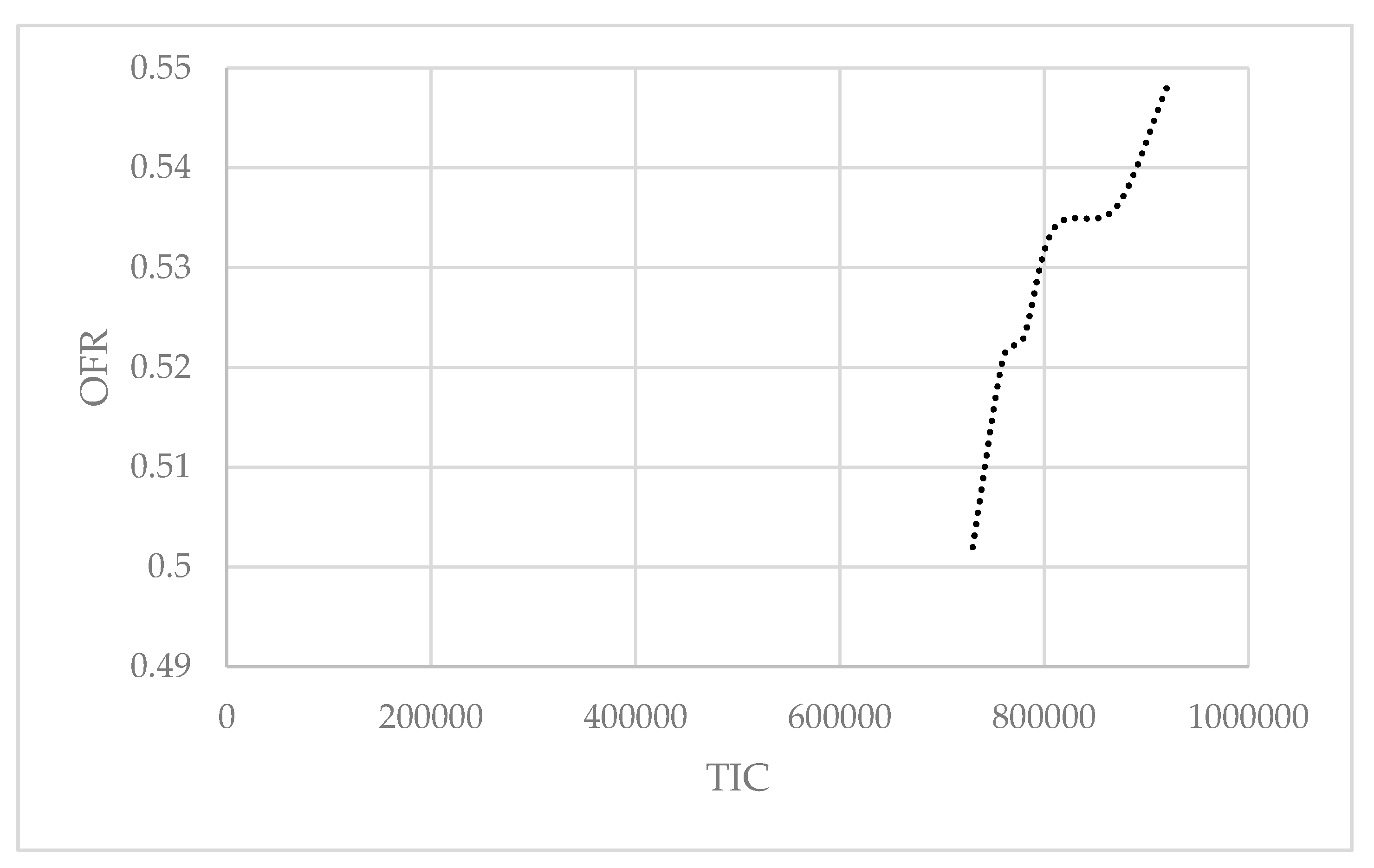
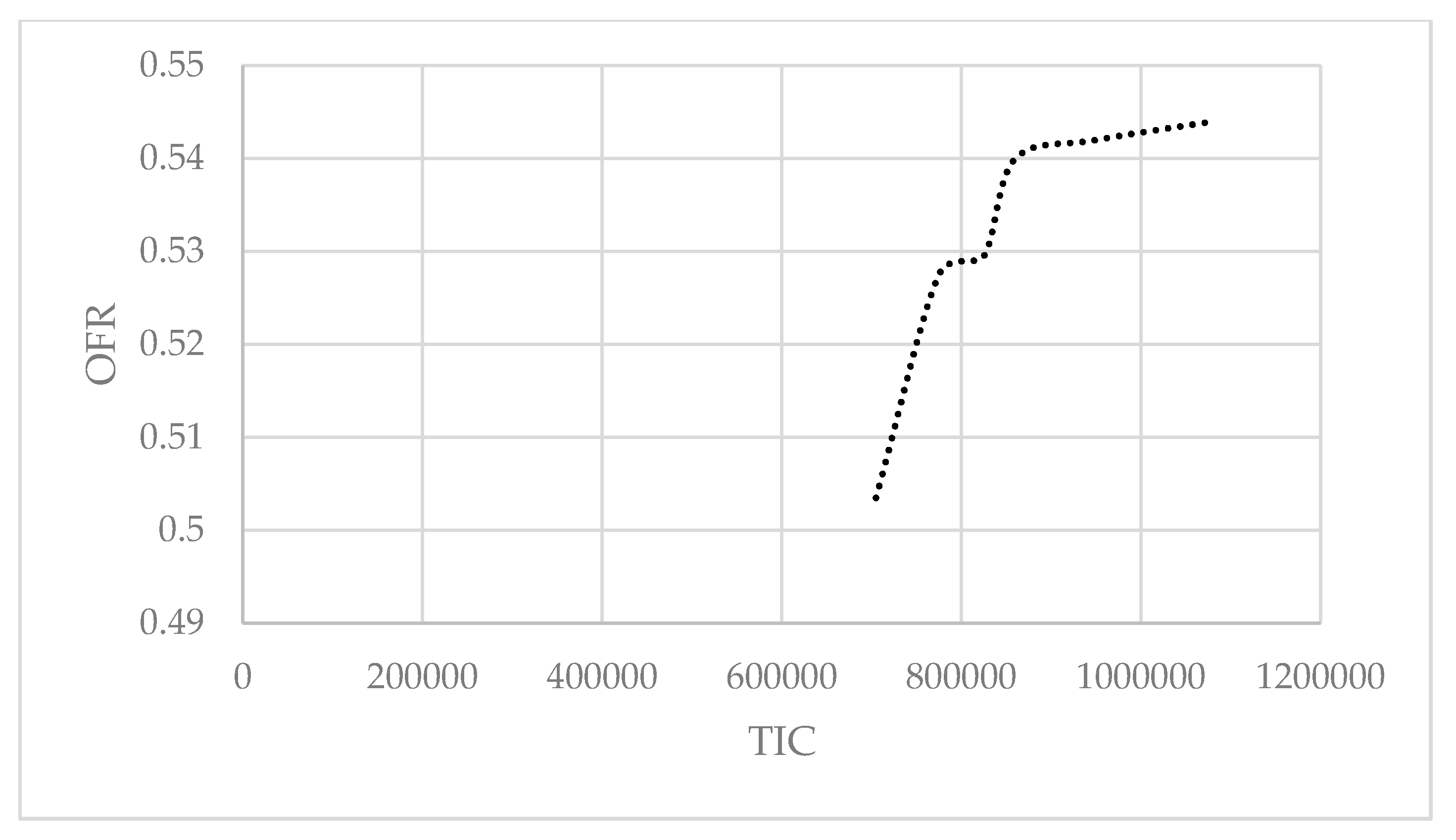
As already mentioned, the purpose of this simulation is to test the case in which the information from the end-customer is used regarding two scenarios: (1) when the relative weight of the expected demand information of $\mathsf{\theta }$ is automatically adjusted from 0 to 1, and (2) when the relative weight of the expected demand information of $\mathsf{\theta }$ is fixed to 0. The simulation results are plotted in Figure 5 and Figure 6, and the specific values are summarized in

Table 6. Ranges of total inventory cost and order fill rate considering the level of information quality under information sharing conditions.

	$\mathsf{\theta }$	$\mathsf{\theta }\le 0$	$\mathsf{\theta }=1$
Objective Function
Total inventory cost	Min	707,502.4	747,763.7
	Max	1,072,705.1	909,893.5
Order fill rate	Min	0.503	0.502
	Max	0.543	0.548

.

As shown in Table 6, the TIC for $\mathsf{\theta }\le 1$ was between 707,502.4 and 1,072,705.1, whereas for $\mathsf{\theta }=0$, the TIC was between 747,763.7 and 909,893.5. The ranges of the OFR for $\mathsf{\theta }$ fixed at 0 and $\mathsf{\theta }\le 1$ were 0.502 to 0.548 and 0.503 to 0.543, respectively.

A detailed comparison of the TIC for both scenarios is shown in

Table 7. Statistical analysis of total inventory cost under information sharing conditions.

Factor	N	Total	Mean	Variance
TIC($\mathsf{\theta }\le 1$)	200	168517700	842,588.4999	15,474,607,605
TIC($\mathsf{\theta }=0$)	200	161474921	807,374.6062	3,400,844,185

.

As shown in Table 7, the mean and variance of the TIC were 842,588.4999 and 15,474,607,605, respectively, when θ was automatically adjusted. When θ was zero, the mean and variance of the TIC were 807,374.6062 and 3,400,844,185, respectively. The ANOVA test at a 0.05 level of significance was performed to identify whether any significant difference in the TIC existed between the two scenarios. The ANOVA test results are summarized in

Table 8. ANOVA test results for total inventory cost under information sharing conditions.

Cause of Variance	Sum of Squares	df	Mean Square	F	Sig.	Pr > F
Treatment (factor)	1.24002 × 1011	1	1.24002 × 1011	13.13895233	0.0003267	3.8649292
Residual	3.75621 × 1012	398	9437725895
	3.88022 × 1011	399

.

As shown in Table 8, since p = 0.0003267, the p-value was lower than the α-level. Thus, it can be concluded that there was a difference between adjusting θ and fixing θ. Consequently, the TIC varied according to the relative weight of the expected demand information.

Furthermore, it is necessary to understand the OFRs for both the adjusted θ and fixed-value θ. The results of the statistical analysis of the OFRs are summarized in

Table 9. Statistical analysis of order fill rate under information sharing conditions.

Factor	N	Total	Mean	Variance
OFR($\mathsf{\theta }\le 1$)	200	106.3083	0.531542	0.000163
OFR($\mathsf{\theta }=0$)	200	105.3917	0.526958	0.000205

.

As shown in Table 9, when the $\mathsf{\theta }$ was adjusted from 0 to 1, the mean and variance of the OFR were 0.531542 and 0.000163, respectively. When the value of $\mathsf{\theta }$ was fixed to 0, the mean and variance of the OFR were 0.526958 and 0.000205, respectively. An ANOVA test was also performed at a 0.05 level of significance to find out whether there was any significant difference in the TIC between these two scenarios. The ANOVA test results are summarized in

Table 10. ANOVA test results for order fill rate under information sharing conditions.

Cause of Variance	Sum of Squares	df	Mean Square	F	Sig.	Pr > F
Treatment (factor)	0.002101	1	0.002101	11.42235	0.000797	3.864929
Residual	0.073197	398	0.000184
Total	0.075297	399

.

As shown in Table 10, since p = 0.000797, the p-value was lower than the α-level. Thus, it can be concluded that there was a difference between adjusting θ and fixing θ. Consequently, the level of information quality affects the OFR when end-customer information is shared.

In summary, adjusting the relative importance of the expected demand information has an influence on OFR. The coefficient of variance for adjusting $\mathsf{\theta }$ was 0.024 and for fixing $\mathsf{\theta }$ to 0, it was 0.027. Thus, adjusting the relative weight of the expected demand information is considered to improve and stabilize OFR. In terms of total inventory cost, this adjustment indicates that trusting the level of downstream information quality completely may reduce the bullwhip effect.

The data presented above are rearranged in

Table 11. Statistical information on total inventory cost and order fill rate under both information non-sharing and sharing conditions.

Sharing Condition	Objective Function		$\mathsf{\theta }\le 1$	$\mathsf{\theta }=0.25$
Non-Information Sharing	Total inventory cost	Min	1,424,416.167	1,630,458.682
		Max	1,866,388.589	2,170,367.994
		Mean	1,624,741.998	1,890,626.672
		Variance	2,553,493,5240	39,302,200,428
	Order fill rate	Min	0.478	0.475
		Max	0.537	0.540
		Mean	0.517925	0.5202917
		Variance	0.000289	0002969
			$\mathsf{\theta }\le 1$	$\mathsf{\theta }=0$
Information Sharing	Total inventory cost	Min	707,502.400	747,763.700
		Max	1,072,705.100	909,893.500
		Mean	842,588.4999	807,374.6062
		Variance	15,474,607,605	3,400,844,185
	Order fill rate	Min	0.503	0.502
		Max	0.543	0.548
		Mean	0.531542	0.526958
		Variance	0.000163	0.000205

to compare the two cases of sharing and non-sharing information.

In terms of TIC, adjusting the relative weight of the expected demand information offers a more effective solution in the absence of information sharing, and fixing the relative importance of the expected demand information to zero offers an improved solution when information is shared. To identify whether there was any significant difference in the TIC between these two scenarios, an ANOVA test was performed at a 0.05 level of significance, and the results are summarized in

Table 12. ANOVA test results for inventory holding costs with and without information sharing.

Cause of Variance	Sum of Squares	df	Mean Square	F	Sig.	Pr > F
Treatment(factor)	6.68 × 1013	1	6.68 × 1013	4617.739	4.3 × 10−221	3.864929
Residual	5.76 × 1012	398	1.45 × 1010
Total	7.26 × 1013	399

.

As shown in Table 12, the p-value was lower than the α-level, because p = 4.3 × 10⁻²²¹. Thus, it can be concluded that there is a difference between adjusting the relative weight without information sharing and fixing the relative importance to 0 when information is shared. When comparing the mean values of TIC as shown Table 11, the TIC for adjusting the relative weight without information sharing was 101.2% higher than that for fixing the relative importance with information sharing. The coefficient of variance for adjusting the relative weight without information sharing was 0.098, and the coefficient of variance for fixing the relative importance to 0 with information sharing was 0.072. Thus, fixing the relative weight of the expected demand information to 0 can be considered to be more stable.

Consequently, adjusting the initial conditions and the relative weight of the expected demand information offers a better solution than fixing the initial conditions by referring to existing valid values when information is not shared via the supply chain. When information sharing is allowed, fixing the relative importance of the expected demand information to 0 offers a more optimal solution than adjusting the relative weight, although the TIC only improved by 4.2%. This suggests that the proposed optimization method is as efficient as the method that uses 100% of information from the end-customer.

5. Discussion

A supply chain is affected by the extent to which information from downstream tiers is shared. The current study introduced a method that automatically adjusts the conditions by considering the level of information shared in terms of TIC and OFR in the supply chain. The TICs and OFRs were analyzed with and without end-customer information sharing. Without information sharing, viz. adjusting and fixing the relative weight of the expected demand information, different levels of information quality were developed. Likewise, these two scenarios were also investigated under information sharing conditions. The best solutions for information sharing and non-sharing were also compared in terms of TIC.

When comparing the best solution for information sharing with that of information non-sharing, the ANOVA test showed that there is evidence of a significant difference between the total inventory cost of adjusting the relative weight of the expected demand information without information sharing and that of fixing the relative weight of the expected demand information to 0 with information sharing at a 0.05 level of significance. The TIC of adjusting the relative importance without information sharing was higher than that of fixing the relative importance to 0 with information sharing. Additionally, fixing the relative weight to 0 with information sharing offers a more stable solution than adjusting the relative weight without information sharing because the coefficient of variance for fixing the relative importance to 0 is smaller than that of adjusting the relative importance.

Consequently, adjusting the relative weight of the expected demand information offers an improved solution without information sharing, and fixing the relative importance of the expected demand information to 0 improves the solution when sharing information. Furthermore, adjusting the relative importance could still be considered to be more efficient than the proposed method, although the scenario of fixing the relative importance produces an improved solution when sharing information.

6. Conclusions

The current study suggested a method for supply chain optimization by considering the conditions and level of information quality under conditions of information sharing and non-information sharing. In this regard, PSO was applied as the algorithm for supply chain optimization, and OFR and TIC were used as objective functions. The customer demand was assumed to be the AR (1) model with normal distribution $\mathrm{N}\left(0,{\mathsf{\sigma }}^2\right)$ with a mean value of 0, standard deviation ${\mathsf{\sigma }}^2$, and $\mathsf{\rho }$ as the first-order autocorrelation coefficient. Both information sharing and non-sharing were compared, and the level of information sharing, expressed as the θ value, was adjusted while performing supply chain optimization.

In conclusion, this study performed an overall optimization of the supply chain to satisfy the objective functions TIC and OFR when the θ value, which means the level of information sharing in the upstream and downstream tiers of the supply chain, is fixed and varied. When the information was not shared, when the θ value was changed, it was superior to when it was fixed. When information sharing was permitted, θ = 1 was better than when it was changed, but there was no significant difference. The effect of the level of information sharing on the objective functions TIC and OFR was analyzed using ANOVA and was found to have a significant effect on OFR and TIC.

Since the level of information sharing depends on factors and effects associated with the supply chain, it may be necessary to not only consider end-customer information, but also various other forms of information in the supply chain.