Research on Shear Behavior and Crack Evolution of Symmetrical Discontinuous Rock Joints Based on FEM-CZM

Abstract

The discontinuous joints are an essential type of natural joints. The normal force, joint persistency, and distribution exert great influences on the shear resistance of the rock joints. By simulating the uniaxial compression experiment and Brazilian test, the material parameters and the basic size standard for meshing were determined. The symmetrical discontinuous joint distribution of three types were established, the cohesive elements were inserted between the solid elements, and the numerical simulation of the shear test was conducted. The effects of joint distribution, joint continuity, and normal stress on the shear resistance of joint rock were investigated, and the law of crack evolution was analyzed. The results showed that the shear process of discontinuous joints can be divided into four stages: elastic stage, strengthening stage, plastic stage, and residual stress stage. For the scattered joint distribution, the rock bridge can provide more reinforcement for the joints, which enhances the shear resistance of the joints, the stress concentration point at the end of the joint is easy to accumulate more fracture energy, which induces the initiation of the cracks, and under the influence of unbalanced torque, the both-sided joint distribution is more likely to produce tension damage.

1. Introduction

In nature, when deformed to a certain degree, the rock mass is no longer continuous and intact, with cracks of different sizes initiated inside. If there is no significant displacement of the rock mass on both sides of the fracture surface, the crack surface is called the joint. A lot of engineering projects have shown that the joint features the weak part of the natural rock mass, and the natural rock mass failure starts from the joints [1,2,3,4,5]. The evolution, distribution, lengths, and mechanical properties of joints affect the stability of rock mass. From the perspective of engineering application, the jointed rock mass can be divided into the rock mass with continuous joints and the rock mass with discontinuous joints. Discontinuous joints are commonly seen in nature. The discontinuous joint rock mass contains rock bridge and joints, whose responses under mechanical conditions constitute the overall mechanical properties of the discontinuous joint rock mass. The mechanical properties, deformation characteristics, and crack evolution characteristics of the discontinuous joints are closely related to their size, density, and spatial distribution characteristics [6]. For underground geotechnical engineering, the study on the shear characteristics of symmetrical discontinuous joints will provide a basis for the reinforcement and support design of jointed rock mass.

Many theoretical, experimental, and numerical simulation studies have been carried out on the jointed rock mass [7,8,9,10,11]. The formula for calculating the shear strength of the discontinuous joints based on the Mohr-Coulomb criterion serves as a guide for engineering applications. Lajtai [12] divided the failure modes of the rock bridge into three types: tensile, shear, and ultimate, through extensive experiments and theoretical studies, and proposed corresponding failure criteria. The Jennings criterion [13], due to its simultaneous consideration of the resistance of rock bridges and joints to shear, has been widely used in engineering practices. Yang et al. [14] discussed the effects of joint persistence and the UCS/Ts (the ratio of unconfined compressive strength to tensile strength) ratio on the shear properties of the discontinuous joints through laboratory tests and numerical simulations. They discovered three failure modes, including the tensile failure, the shear failure, and the compressive-shear failure. With the rapid development of computer technology, the numerical simulation has been widely used in the studies on the mechanical properties and crack evolution of brittle rock mass [15,16,17]. Based on the different assumptions about the rock mass continuity, the numerical simulation technologies are divided into continuum- and discontinuous-based methods [18,19,20]. Based on the assumption of the discontinuous medium, the discrete element method (DEM), by solving the equation of motion, achieves the simulation of elastic dynamics such as stress field evolution and acoustic emission. During the process, the particle flow code (PFC) can well simulate the crack evolution and energy diffusion of the rock mass and the flow displacement of the particles by setting certain mass or physical and mechanical parameters to the disc or sphere [21,22,23,24]. Though the discrete element technology can effectively simulate the process of crack evolution of brittle materials [25,26], it still has great difficulty in objectively describing the internal micro-geometric characteristics of the rock mass fracture process [27], with low computational efficiency of the discrete element, which fails to deliver satisfactory performance in engineering practices. In addition to the discrete element technology, the finite element method (FEM) based on the continuum assumption has also been employed to the studies on the dynamic fracture and deformation of rock masses [28,29,30]. However, in the dynamic simulation of large deformation, the reconstruction of element deformation and mesh requires a large amount of calculation, which, to a certain extent, is unable to reflect the dynamic fracturing and crack evolution process of the rock mass [31]. To solve these defects facing the finite element method, many scholars have attempted to improve it, such as the extended finite element method (XFEM) [32,33] and the generalized finite element method (GFEM) [34]. However, the finite element method based on the continuum medium is still unable to simulate the microstructural damage of the materials well.

Considering that the rock mass cannot be simply divided into continuous or discontinuous mass, but a combination of them instead [35], and also for overcoming the deficiencies of discrete elements and finite elements, the scholars began to adopt the finite element-discrete element coupling method (FDEM) [36] in engineering projects such as roadway excavation and support [37,38], surrounding rock reinforcement [39], and slope stability analysis [40]. Dugdale [41] and Barenblatt [42] proposed a new theoretical model named the cohesive zone model (CZM), which considers the microstructure of the rock material and enables the demonstration of rock discontinuity and the simulation of the crack initiation and evolution process of brittle materials. Yang et al. [43] developed an algorithm that can insert the zero-thickness cohesive element into solid finite element mesh, thereby forming a potential crack surface in the model, which provides the possibility of achieving complex crack evolution. Jiang et al. [44] inserted the cohesive element into the finite element, established a three-dimensional numerical model to investigate the fracture, penetration, and the chip shape of the rock during cone rock breaking, and discovered through comparison that the numerical simulation shares great similarity with laboratory tests in results. Chang et al. [45] established a two-dimensional Brazilian test model and embedded a zero-thickness cohesive element to investigate the complex crack behaviors in a layered disc with interfacial cracks. Through the comparison between their results with those obtained in laboratory tests, it was found that they are quite consistent in crack development mode and mechanical properties. Besides, they analyzed the mesh sensitivity of cohesive elements. Haddad et al. [46] established a two-dimensional hydraulic fracturing model and analyzed the effects of the initial crack length and mesh refinement on calculation convergence. Wang et al. [47] used the CZM to model the shearing process of bolted jointed rock. The numerical model is verified by the comparison with the experiment results, which demonstrated that it can be effectively applied to the simulation of joint shearing process. Han et al. [48] studied the shear behavior of rock-like materials with cracks by using the FEM-CZM method. The mechanical properties, shear deformation, and cracking behaviors of specimen were respectively discussed.

At present, considering the discontinuity of the jointed rock mass, most scholars prefer to use discrete element software to simulate the shear of discontinuous joints, and it is relatively rare to use the FEM-CZM method. This paper adopted the finite element software ABAQUS to establish shear models with different joint persistence, densities, and spatial distributions, and inserted cohesive elements thoroughly to generate potential crack surfaces inside the model. By simulating the uniaxial compression test and the Brazilian test, and comparing the results with those by laboratory experiments, we determined the material parameters and the basis for mesh division. In addition, we investigated the effect of joint distribution, joint persistence, and normal stress on the shear resistance of rock, and analyzed the crack evolution law during the shear process of discontinuous joints of three different distribution forms.

2. FEM-CZM Simulation of Rock Shear

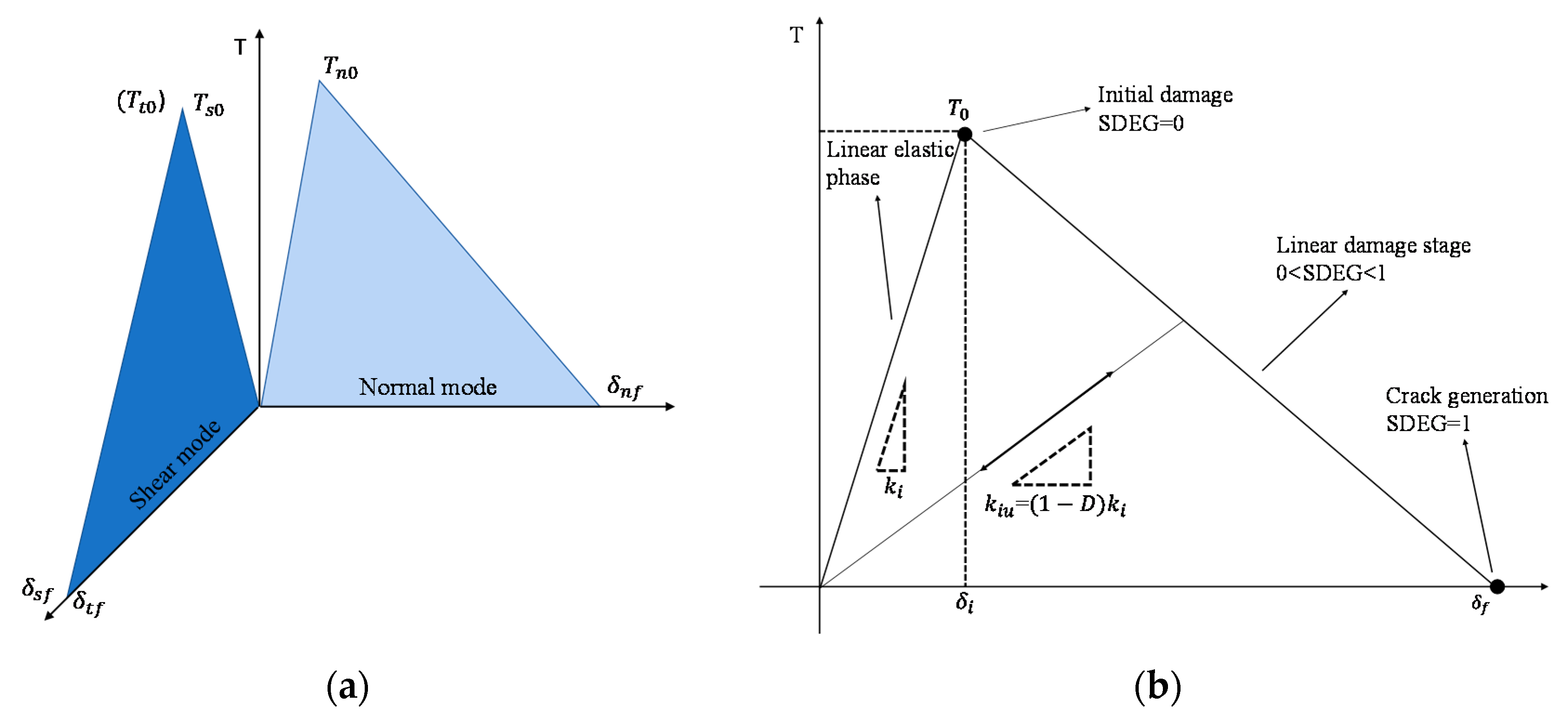
2.1. Initial Linear Elastic Traction-Displacement

Several constitutive relationships of the CZM have been developed on the basis of an effective displacement and an effective traction, and different constitutive models have their own applicable conditions [49]. Cong [50] discovered that the energy-based Separation-Traction linear model (S-T model) delivers better performance in simulating fracture of brittle materials with good applicability. Alfano [51] concluded that the S-T linear model features better simulation accuracy and calculation efficiency through comparative analysis. Therefore, this paper selected the S-T linear model as the criterion for the damage of cohesive elements, whose constitutive relationship is shown in Figure 1.

The S-T model includes two stages: (1) the linear elastic stage, in which no damage occurs to the cohesive element and the element stiffness remains constant, and (2) the linear damage stage, in which the cohesive element damage evolves, and the element stiffness decreases continuously. In the first stage, we can use a matrix containing nominal strain and nominal stress for description. In order to facilitate parameter calibration, the constitutive thickness of the cohesive element was set to 1, and the geometric thickness was set to 0 by default, which can make the node separation displacement equal to the nominal strain. The elastic stage of the S-T criterion can be expressed as:

$$t=\left\{\begin{array}{c}{t}_n\\ t_s\\ t_t\end{array}\right\}=\left[\begin{array}{ccc}{E}_{nn}& E_{ns}& E_{nt}\\ E_{ns}& E_{ss}& E_{st}\\ E_{nt}& E_{st}& E_{tt}\end{array}\right]\left\{\begin{array}{c}{\epsilon }_n\\ {\epsilon }_s\\ {\epsilon }_t\end{array}\right\}=E\epsilon =\frac{1}{T_0}K\delta$$

(1)

where $t$ is the nominal traction stress vector consisting of three components, $t_n$, $t_s$, and $t_t$, $\epsilon$ is the nominal strain consisting of ${\epsilon }_n,$ ${\epsilon }_s,$ and ${\epsilon }_t$, $T_0$ is initial thickness of the cohesive element, δ is the displacement of the cohesive element, and K is the corresponding stiffness matrix.

2.2. Linear Damage Stage of Cohesive Element

It was assumed that there are three traction forces on the crack surface, namely the normal traction force $t_n$ and two tangential traction forces $t_s$ and $t_t$, all of which gradually decrease as the crack propagates. When the traction force becomes 0, the element will be wholly damaged. This study utilized type I and type II fracture to study the rock properties. The fracture energy can be represented by the triangular area in Figure 1a, which is type I fracture energy and type II fracture energy, respectively.

Describing the damage evolution process of cohesive elements entails at least three of the four parameters, including the initial stiffness, $K_0$, the ultimate strength, $t_0$, the critical fracture energy, $G_f$, and the final failure displacement, ${\delta }_f$. In this paper, we selected $K_0$, $t_0$, and $G_f$ as the research parameters. The quadratic nominal stress criterion (QUADS) was used for judging the start of damage evolution, and, according to it, the damage starts to evolve when the quadratic interaction function involving the nominal stress ratios (as defined in the expression below) is equal to 1.

$${\left\{\frac{<t_n>}{t_{n0}}\right\}}^2+{\left\{\frac{t_s}{t_{s0}}\right\}}^2+{\left\{\frac{t_t}{t_{t0}}\right\}}^2=1$$

(2)

where the < > is a Macaulay bracket, which ensures that the damage evolution only occurs under the action of forwarding tension and the compressive stress will not cause damage to the cohesive element. The QUADS criterion ensures that the damage of the cohesive element be generated under the combined action of normal stress and tangential stress.

To describe the degree of damage evolution, we introduced a damage variable, D, the value of which gradually changes from 0 to 1 as the load increases. When D reaches 1, the cohesive element also reaches the ultimate bearing capacity with the cohesive element automatically deleted, and the free edges are formed in the continuously arranged elements, which means the cracks are initiated. The calculation of the damage variable, D, is shown as follows:

$$D=\frac{{\delta }_{mf}\left({\delta }_m-{\delta }_{m0}\right)}{{\delta }_m\left({\delta }_{mf}-{\delta }_{m0}\right)}$$

(3)

where ${\delta }_{mf}$ is the corresponding displacement at the moment of complete failure$, {\delta }_{m0}$ is related to the displacement at damage initiation, and ${\delta }_m$ denotes the maximum displacement attained during the loading, which is expressed below:

$${\delta }_m=\sqrt{{<{\delta }_n>}^2+{\delta }_s{}^2+{\delta }_t{}^2}$$

(4)

Therefore, the changes of the parameters of the T-S model with the cumulative damage are as follows:

Traction:

$$t_n=\{\begin{array}{ll}\left(1-D\right)t_{n0},& t_{n0}\ge 0\\ t_{n0},& t_{n0}<0\end{array}$$

(5a)

when $t_{n0}$ < 0, there is no damage.

$$t_s=\left(1-D\right)t_{s0}$$

(5b)

$$t_t=\left(1-D\right)t_{t0}$$

(5c)

Stiffness:

$$k_n=\left(1-D\right)k_{n0}$$

(6a)

$$k_s=\left(1-D\right)k_{s0}$$

(6b)

$$k_t=\left(1-D\right)k_{t0}$$

(6c)

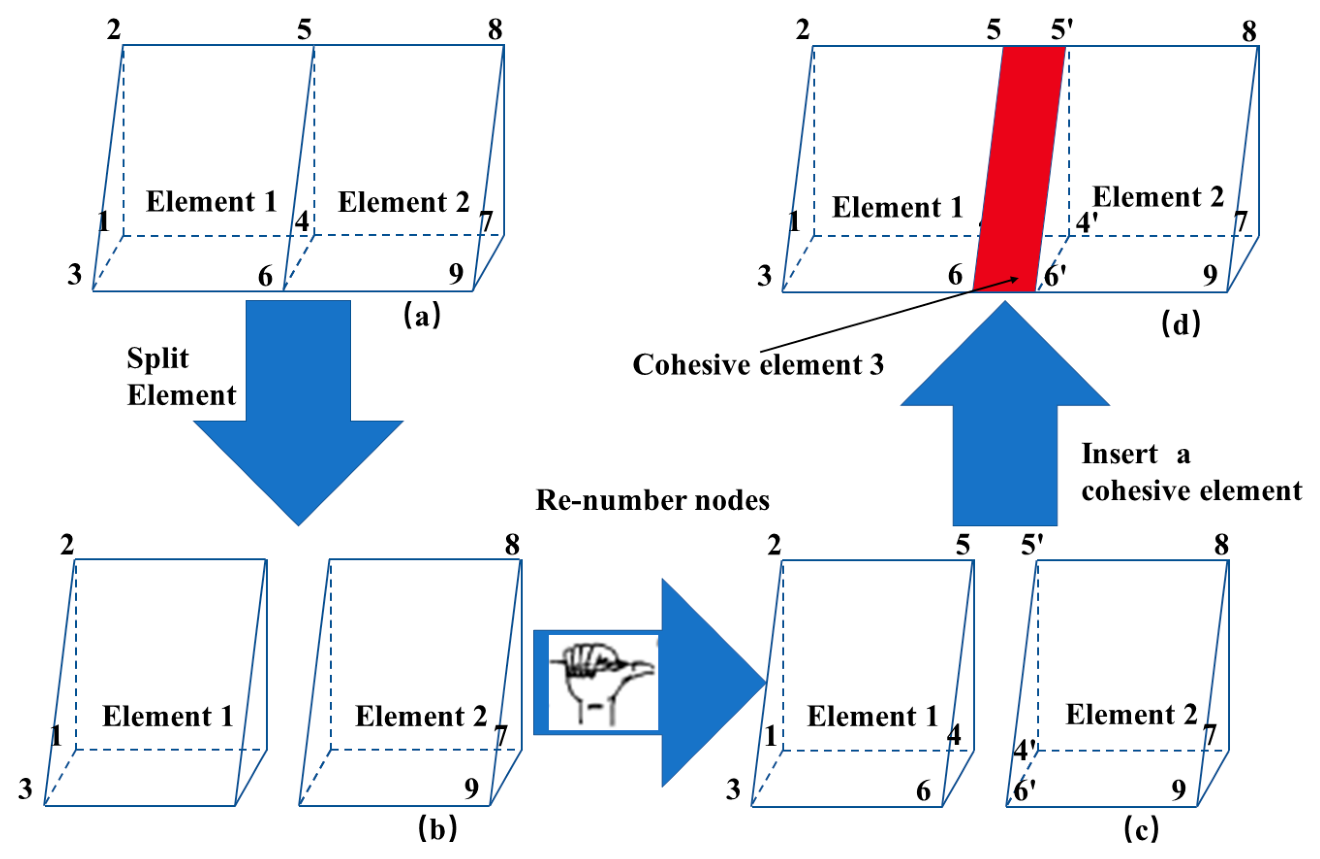
2.3. Cohesive Element Inserting Process

In order to simulate the random development progress of cracks, the cohesive element was inserted into the solid elements to form a potential crack surface. In the simulation model, the solid discrete elements form a continuum through zero-thickness cohesive elements. The top and bottom surfaces of each zero-thickness cohesive element are connected to the solid element, with the nodes shared. The process of embedding cohesive elements is shown in Figure 2. The node renumbering follows the right-hand rule to ensure that each node has a unique number. Since the model has a large number of solid elements, it is infeasible to manually insert cohesive elements. Therefore, a calculation program was developed based on the Python language, which can automatically insert cohesive elements into the solid elements.

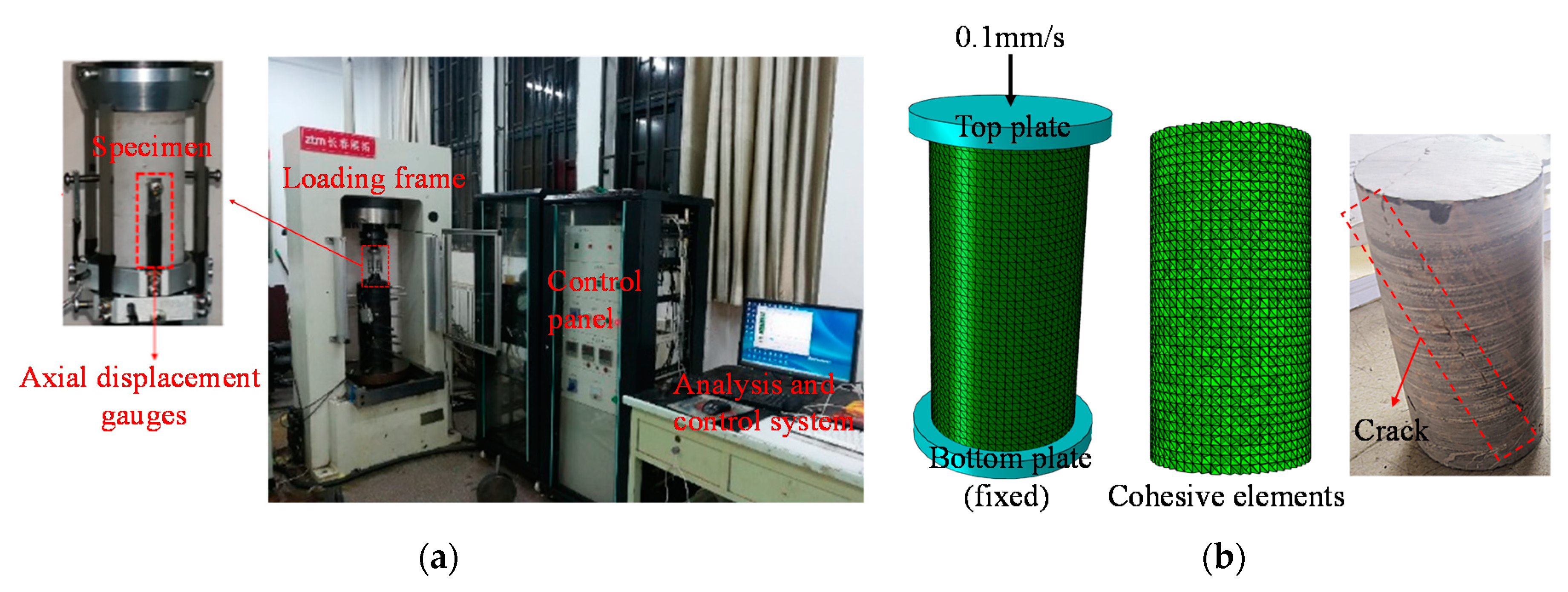
3. Model Establishment

3.1. Parameters Determination

To obtain the main mechanical parameters of sandstone, according to the recommendations of the International Society for Rock Mechanics (ISRM), we prepared a cylindrical specimen with the diameter of 50 mm and the height of 100 mm for the uniaxial compression test, as shown in Figure 3a. The loading rate was set to 0.01 mm/min and we stopped the loading after the test piece was obviously damaged and the loading curve exceeded the peak [52]. During the test, we kept other variables unchanged and did not apply the confining pressure. Then, we established a three-dimensional uniaxial compression numerical model with the same dimensions as the laboratory experiment, which was inserted into the cohesive element by the finite element plug-in. Besides, we set a loading plate, which was given the stiffness much higher than that of the specimen, to ensure that the load can be evenly applied on the top of the test piece, as shown in Figure 3b. When the lower loading plate was fixed, the upper one moved downward at a speed of 0.1 mm/s until the specimen was destroyed. Under ideal conditions, the numerical simulation should set the same loading speed as the laboratory experiment, which, however, requires a smaller time step and longer calculation time. Thus, we amplified the loading speed by ten times. Through the parameter comparison, the parameters of cohesive elements were determined. Multiple sets of parameters were used for simulation, whose results were compared with those obtained by laboratory experiment. If the parameters are similar, the parameters are considered to be finally determined.

After many attempts, the uniaxial compression numerical model obtained the mechanical properties and crack evolution characteristics of the numerical simulation similar to the laboratory experiment, as shown in Figure 4. It can be found from the results that the peak compressive strength of the laboratory experiment is 43.4 MPa with the corresponding axial strain being 0.41%, while the peak compressive strength of the numerical simulation is 45.6 MPa with the corresponding axial strain being 0.43%, both of which are very close. Both of the stress-strain curves obtained from the numerical simulation and the laboratory experiment show a trend of sudden stress drop after reaching the peak.

At the same time, through a summary of the crack evolution process in the numerical simulation, we found that the small cracks first appeared in the middle part of the specimen. As the axial load increased, the small cracks further propagated, gradually connected with each other, and finally formed the main fissure penetrated through the specimen. This phenomenon is the same with the uniaxial compression crack growth process observed by Basu et al. [53]. Simultaneously, we monitored SDEG, defined as the scalar stiffness degradation variable of the cohesive element during the uniaxial compression process, which can reflect the damage degree of the cohesive element. It can be found that the damage of the cohesive element derived from the inner part of the specimen, and under the action of tensile stress, extended along the diagonal of the specimen and eventually penetrated the entire specimen. This process corresponds to the crack propagation process. The comparison between the results of the numerical simulation and those of the laboratory experiment reveals the reasonableness of the selection of the parameters. The final parameters of the numerical simulation element are shown in

Table 1. Numerical simulation material parameters.

Materials	Parameters	Value
Solid element	Density (kg·m−3)	2.5 × 10 3
	Young’s modulus (GPa)	15
	Poisson’s ratio	0.3
Cohesive element	Initial tensile stiffness (GPa·m−1)	15
	Initial shear stiffness (GPa·m−1)	5.28
	Normal traction force (MPa)	6
	Tangential traction force (MPa)	22
	Model-I fracture energy (N·mm−1)	6 × 10−2
	Model-II fracture energy (N·mm−1)	1.65 × 10−1
Loading plate	Density (kg·m−3)	7.8 × 10 3
	Young’s modulus (GPa)	2.1 × 10 2
	Poisson’s ratio	0.3

.

Since the crack evolution characteristics and mechanical characteristics of the specimen are closely related to the size of the cohesive element, it is necessary to perform the mesh sensitivity analysis of the specimen. As shown in Figure 5a, a two-dimensional Brazilian test numerical model was established with the disc’s diameter of 50 mm and the plane’s outer thickness of 40 mm. The sizes of the mesh sizes were set respectively to 0.5, 1, 2, and 3 mm to carry out the Brazilian test simulation, through which we obtained the load-displacement curve in the process of simulation, as shown in Figure 6. With the mesh of 1 mm, when the normal displacement is 0.39 mm, the maximum load along the normal direction is 9.85 kN, while the peak value of the load obtained in the laboratory experiment is 10.0 kN with the corresponding normal displacement of 0.41 mm. Besides, we obtained the final fracture form of the numerical simulation specimen, as shown in Figure 5b, which is similar to the laboratory experiment result and consistent with the research of Chang et al. [44]. It was found that after the load reached the peak, a vertically penetrated fissure was generated in the middle of the specimen. Therefore, we set the mesh size to 1 mm, with the consideration of the calculation efficiency.

3.2. Model Establishment

Since the shear-induced cracks can cause collision and misalignment between the elements, we adopted global contact to define the contact behaviors. The global contact algorithm, however, can only be applied to the three-dimensional surface contact, thus we utilized a three-dimensional model for analysis. A model with the dimensions of 200 × 100 × 1 mm was established, and the zero-thickness cohesive elements were inserted into the specimens, as shown in Figure 7. During the numerical simulation, we simulated the loading process of the shear box through setting appropriate boundary conditions. During the shearing process, we applied a constant normal load, $\mathsf{\sigma },$ to the top and an appropriate shear speed, $\mathsf{\tau },$ to the upper part, with the lower part remaining static.

To accurately describe the characteristics of the discontinuous joints, we introduced the joint persistence, $p_j$, as shown below:

$$p_j=\frac{2L_j}{2L_j+L_r}=\frac{2L_j}{L}$$

(7)

where $L_r$ is the length of the rock bridge, and $L_j$ is the length of the joint.

In this paper, 0 < $p_j$ < 1, which means that all the specimens are composed of joints and rock bridges.

To analyze the effect of the discontinuous joint distribution, joint persistence, and normal stress on the shear resistance of rock, we established joint distribution models of three types, namely, both sided (type-I), scattered (type-II), and central (type-III), as shown in Figure 8. Among them, only the type-I joints are open, and there are two discontinuous joints in the type-II and type-III, both of which share the same length (joint persistence) and are symmetrical about the central axis. We set three normal stresses of 0.5, 1.0, and 1.5 MPa respectively, and set four different joint persistences of 0.2, 0.4, 0.6, and 0.8 respectively, with the corresponding rock bridge lengths of 160, 120, 80, and 40 mm. In this paper, a total of 36 discontinuous joint shear models under different conditions were established. It should be stated that this paper did not take consideration of the effect of shear rate on shear performance. The displacement method was used to control the application of the shear load. The shear rate was set to 0.06 mm/min to ensure that the shear be performed under quasi-static conditions. Since the model owns a large number of calculation elements, in order to improve the calculation efficiency, we set a dynamic explicit step and employed the mass scaling technology, which can change the discrete mass matrix by setting mass scaling factor, leading to a corresponding improvement in the calculation efficiency. Mass scaling mainly affects the inertial force of the element; especially, the generated virtual inertial force can easily affect the calculation accuracy and convergence. For quasi-static simulations, it is usually necessary to ensure that the ratio of kinetic energy to potential energy do not exceed 0.1. The load application method adopted in this paper can satisfy this condition.

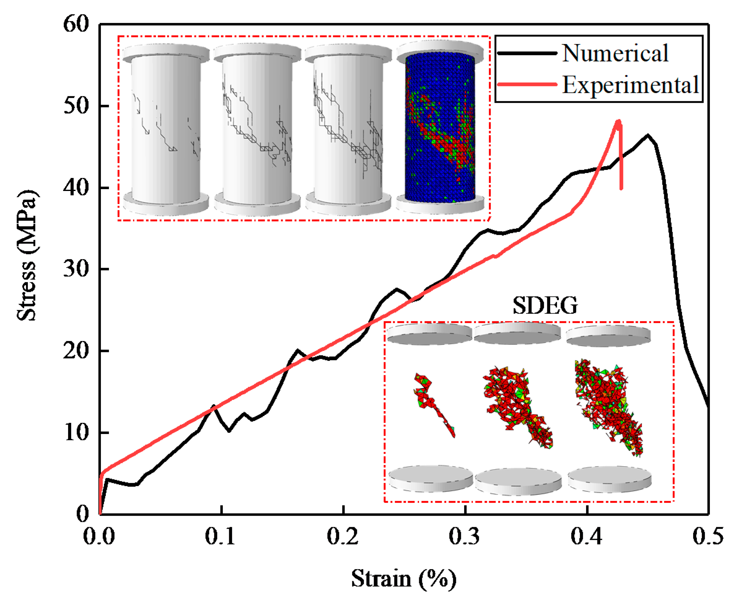
4. Simulation Results and Analysis

4.1. Influence of Joint Distribution on Shear Resistance

The stress-strain curves of the specimens with the persistence of 0.2 are shown in Figure 9. It can be divided into the elastic stage, strengthening stage, plastic stage, and residual stress stage (I–IV). By comparing the curves with different normal stresses, it can be found that the elastic modulus does not change with the variation of the normal stress (I), as proved by the fact that the change of normal stress has little effect on the elastic stage. During this stage, the cohesive elements remained intact with no crack appearing on the specimen. As the shear load was applied, the shear curve enters the strengthening stage (II), and the curve slope increases with the increase of normal stress. During this stage, part of the cohesive elements began to enter the linear damage stage (0 < D < 1), with the damaged cohesive elements (D = 1) deleted and initial cracks appearing. It is worth noting that the local failure of the specimen induced the sudden reduction of the shear resistance, which is shown as a sudden variation of the stress-strain curve in Figure 9a,c. As the shear load increases further, the curve enters the plastic stage (III). During this stage, the cracks further propagated, the shear resistance of the specimen began to decrease, and the peak shear stress showed a positive correlation with the normal stress. As the crack propagated further to form a continuous fissure, the curve enters the residual stage (IV). During this stage, the shear strength is provided by the mechanical bite force and the friction of the test piece.

Comparing the peak strength of joints with different distributions, as shown in Figure 10a, it was found that the shear strengths of the type-II and type-III are the highest, with that of the type-I being the lowest. Stress concentration tends to occur at the ends of joints, from which the cracks are generated and propagated. Compared with the type-II and type-III, the type-I is more likely to produce tensile fractures at the joint ends, resulting in tensile cracks. As the cracks gradually extend through the rock bridge, the specimen enters the residual strength stage. Though the cracks of the type-II and type-III also start from the joint end, they can result in shear failure. Since the rock is more resistant to shear than the tension, the type-I cracks grow with the highest speed, also the specimen enters the residual strength stage. The difference between the strength peak and the residual strength was analyzed, as shown in Figure 10b. It was found that the type-II intensity decreased the most, followed by the type-III, and the type-I decreased the least. In the stress-strain curve, the type-II residual strength stage has a higher slope. It can be seen that type-II features the highest brittleness, while type-I features the highest plastic properties. This is due to more dispersed distribution of the type-II joints and more joint reinforcement provided by the rock bridge, thereby restraining the deformation of the specimen under the shear load. When the shear stress reaches the peak, the penetrated crack is formed in the rock bridge and the accumulated fracture energy is quickly released, making the shear strength decrease more rapidly.

Specimens with the persistence of 0.6 and the normal stress of 1.0 MPa were selected to obtain the vertical displacement field, U2. Figure 11a is the displacement field with no shear load applied, and Figure 11b is the displacement field when the specimen finally fails. The largest vertical displacement always occurs above the joint, while the displacement at the rock bridge is the smallest. During the final failure stage, the vertical displacement of type-I is the largest, while that of type-II is the smallest, which can reflect the degree of the specimen affected by the dilatancy effect. For type-I, since the joints are open, the upper part of the specimen is similar to a cantilever beam, and under normal stress, a negative vertical displacement was generated. During the final failure stage, under the action of the shear stress, a clockwise moment around the centroid of the specimen was generated. Under the effect of the moment, the two ends of the specimen produced vertical displacements in opposite directions. Since the rock bridge can provide a certain degree of reinforcement, the vertical displacement on the side away from the loading site is smaller, and the overall displacement field of type-I is not center-symmetric. For type-II and type-III, during the initial stage, the stress in type-II is more dispersed, making the vertical displacement smaller. During the final failure stage, the whole upper part of the specimen has a positive vertical displacement. In type-II, the three-segmented rock bridge provides more reinforcement for the joint, and the specimen has a smaller deformation. In summary, the type-II has the smallest dilatancy effect during the shearing process, and the specimen has higher rigidity and stability. In comparison, type-I is more likely to produce unbalanced moments, which leads to the instability of the specimen.

4.2. Effect of Joint Persistence on Shear Resistance

Taking the specimen with the normal stress of 1.0 MPa as an example, we investigated the effect of different joint persistence on the joint shear performance. The stress-strain curves of different types of joints distributed under 1 MPa normal stress are shown in Figure 12a–c. With the increase of the joint persistency, the shear stress and shear modulus are gradually decreasing. This is attributed to the fact that the rock bridge provides less reinforcement during the shearing process, with the stiffness of the specimen becoming lower. At the same time, the ratio of peak stress to residual stress gradually decreases, the curves become smoother, and the plasticity of the specimen is higher. The lower the joint persistence is, the steeper the stress-strain curve is, and the more brittle the specimen will be, which shows that the numerical simulation is closer to the direct shear test. The lower joint persistence can result in larger contact area of the specimen after the formation of the penetrated joint, which can provide more friction and mechanical bite force, thus the residual strength of the test piece is higher. The peak shear strengths of these twelve specimens were summarized, as shown in Figure 12d. It can be found that for the specimens with the three joint distribution forms, the peak shear strength and the joint continuity are negatively correlated. The type-II features the highest shear strength with different joint persistence, followed by type-III, and the type-I is the lowest. This shows that with the same overall length of the rock bridge, the scattered rock bridge can play a more significant role in strengthening the joint. In engineering practices, this finding may provide new ideas for strengthening joints by grouting.

We summarized the relationship of the peak shear strength of all specimens with the joint continuity and normal stress, as shown in Figure 13. It can be found that the shear strength of the specimen rises with the increase of the normal stress and drops with the increase of joint continuity. Compared with type-II and type-III, the type-I always has the lowest shear strength. This is because the rock bridge in the type-I cannot provide effective reinforcement for the joints, resulting in the specimen being more prone to fail from the joint tip, especially in the form of tensile failure.

4.3. Crack Evolution Analysis

Under the action of shear load, the cohesive elements fail, and cracks appear on the specimen. The process of crack evolution can reflect the internal mechanical characteristics of the specimen. By modifying the model file, the ratio parameter of the mixed mode of initial damage MMIXDMI is defined. Its initial value was set to –1.0, and it can be expressed as follows:

$$\mathrm{MMIXDMI}=1-m_1$$

(8)

$$m_1=\frac{G_{\mathrm{I}}}{G_T}$$

(9a)

$$m_2=\frac{G_{\mathrm{II}}}{G_T}$$

(9b)

$$m_3=\frac{G_{\mathrm{III}}}{G_T}$$

(9c)

where $G_T$ is the sum of three types of fracture energy, $\mathrm{and} m_1$, $m_2,$ and $m_3$ are the ratios of type I, II, and III fracture energy to total fracture energy, respectively.

Cohesive elements can effectively simulate the three forms of failure, including open cracks, slip cracks, and tear cracks. The last two forms of failure can be collectively referred to as a shear failure. Therefore, we can analyze the driving force for cracking by calculating $m_1$. With the application of shear load, the cohesive elements begin to bear shear stress, tensile stress, or mixed stresses. At this time, $m_1$ changes from 0 to 0.5, the fracture energy accumulated by shearing accounts for most of the total fracture energy of cohesive elements, corresponding to the MMIXDMI value of 1~0.5, and the cohesive elements fail mainly in the form of shear failure. When $m_1$ changes from 0.5 to 1, the fracture energy accumulated by traction accounts for most of the total fracture energy of cohesive elements, corresponding to the MMIXDMI value of 0.5~0, and the cohesive elements fail mainly in the form of tensile failure. In particular, when the value of $m_1$ is 1, 0.5, and 0, the corresponding failure modes of cohesive elements are pure shear failure, tensile-shear failure, and pure tensile failure.

When the joint persistence is 0.6 and the normal load is 1.0 MPa, the stress field S11 of the specimen along the shear direction and the MMIXDMI of the cohesive elements are shown in Figure 14. The crack evolution process of the specimen can be divided into three stages, namely the crack initiation stage (a), crack evolution stage (b), and final failure stage (c).

Firstly, when the shear load is just applied, the cohesive elements begin to accumulate fracture energy. At this time, the cohesive elements are in the linear elastic stage, and the traction force does not reach the initial damage stress, $T_0$. No cracks appear on the specimen, which corresponds to the elastic stage in the stress-strain curve.

As the shear load continues to be applied, the cohesive elements accumulate more fracture energy. Due to the presence of joints inside the specimen, the stress concentration tends to occur at the end of the joint. As shown in Figure 15a, the stress gradually decreases from the joint end to other directions. The cohesive elements near the stress concentration point tend to accumulate more fracture energy, and thus reach the stage of crack evolution, as shown in Figure 15b. The stiffness degradation rate SDEG of the cohesive element at the joint end reaches 1.0 as the first, which is deleted to generate the initial crack, and the specimen enters the crack initiation stage. For the three different types of joint distribution, the initial cracks all appear at the joint ends.

As the load continues to be applied, the tip of the initial crack becomes a new stress concentration point, and the cohesive element at the crack tip quickly reaches the stage of damage evolution, which is thus deleted. The crack continues to grow, and the specimen enters the crack evolution stage. For type-I, the joint ends are more prone to stretching, while for type-II and type-III, the joint ends are more subjected to shearing, thus the crack evolution of type-I joints is faster. Furthermore, under load, the cracks continue to propagate and eventually form the main fissure through the rock bridge, and the specimen enters the final failure stage. At this stage, the type-I joint produces the largest shear deformation, followed by the type-III joint, and the type-II joint has the smallest. Only type-I produces tensile through cracks, which is mainly attributed to the clockwise moment around the centroid of the specimen. For type-II and type-III, the penetrated crack extends along the rock bridge and eventually merges with the joint to form a new joint through the specimen. At this time, the shear resistance of the test piece consists of two parts, one is the mechanical engagement force from the irregular protrusions on both sides of the crack, and the other is the friction resistance on the fracture surface. Through the comparison between the type-II and type-III, it can be found that more cracks are produced on the rock bridge of the type-II joint, and there are even completely free solid elements in the rock bridge on the left, from which it can be inferred that the fracture surface of the type-II rock bridge is rougher.

5. Conclusions

This study used the FEM-CZM method, established the symmetrical discontinuous joint shear model, and inserted cohesive elements into the solid elements to form potential crack surfaces. This method can not only show the mechanical deformation of the element but also have unique advantages in the simulation of complex cracks. Through the uniaxial compression test and the Brazilian tests, we determined the material parameters and the basis for meshing. Three types of discontinuous joints with different distribution forms were established, including both-sided, scattered, and central. The influence of the distribution form, joint persistence, and normal stress on the shear resistance of rock was investigated. The law of crack propagation during the shear process of the joints with three different distribution forms was analyzed. Based on this method, the following main conclusions can be obtained:

(1)

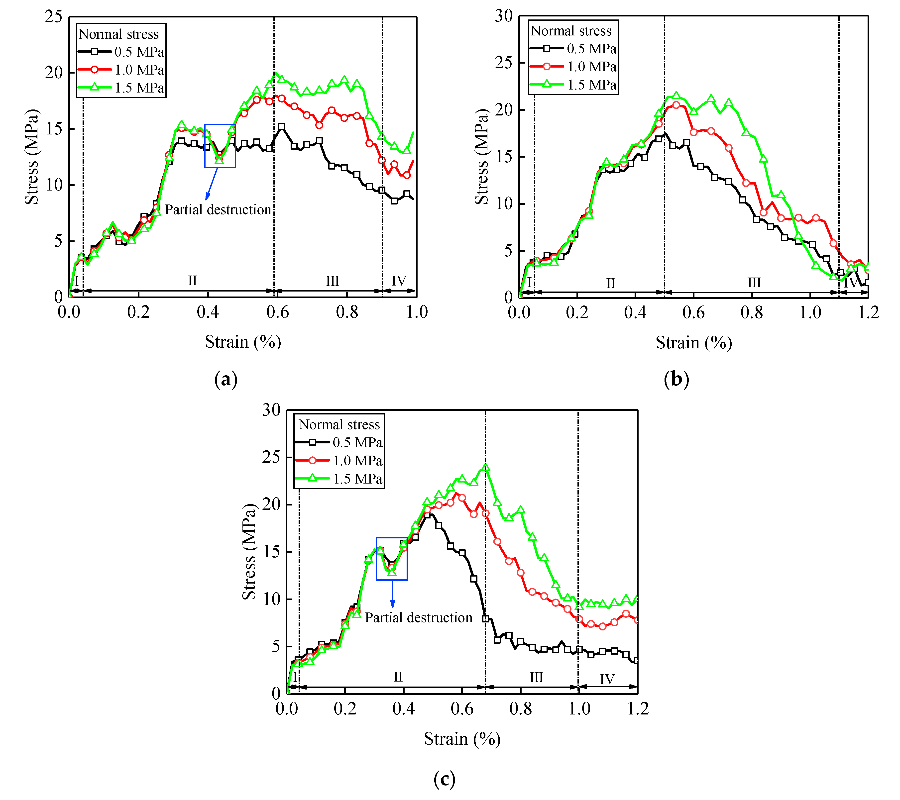
The shearing process can be divided into four stages: elastic stage, strengthening stage, plastic stage, and residual stress stage. In the stress-strain curve, the residual stress stage of type-II has a higher slope, which shows that the type-II has more brittleness and the type-I has higher plasticity. At the same time, with the decrease of joint persistence, the specimen turns more brittle, and the joint shear is closer to the direct shear test of intact rock.

(2)

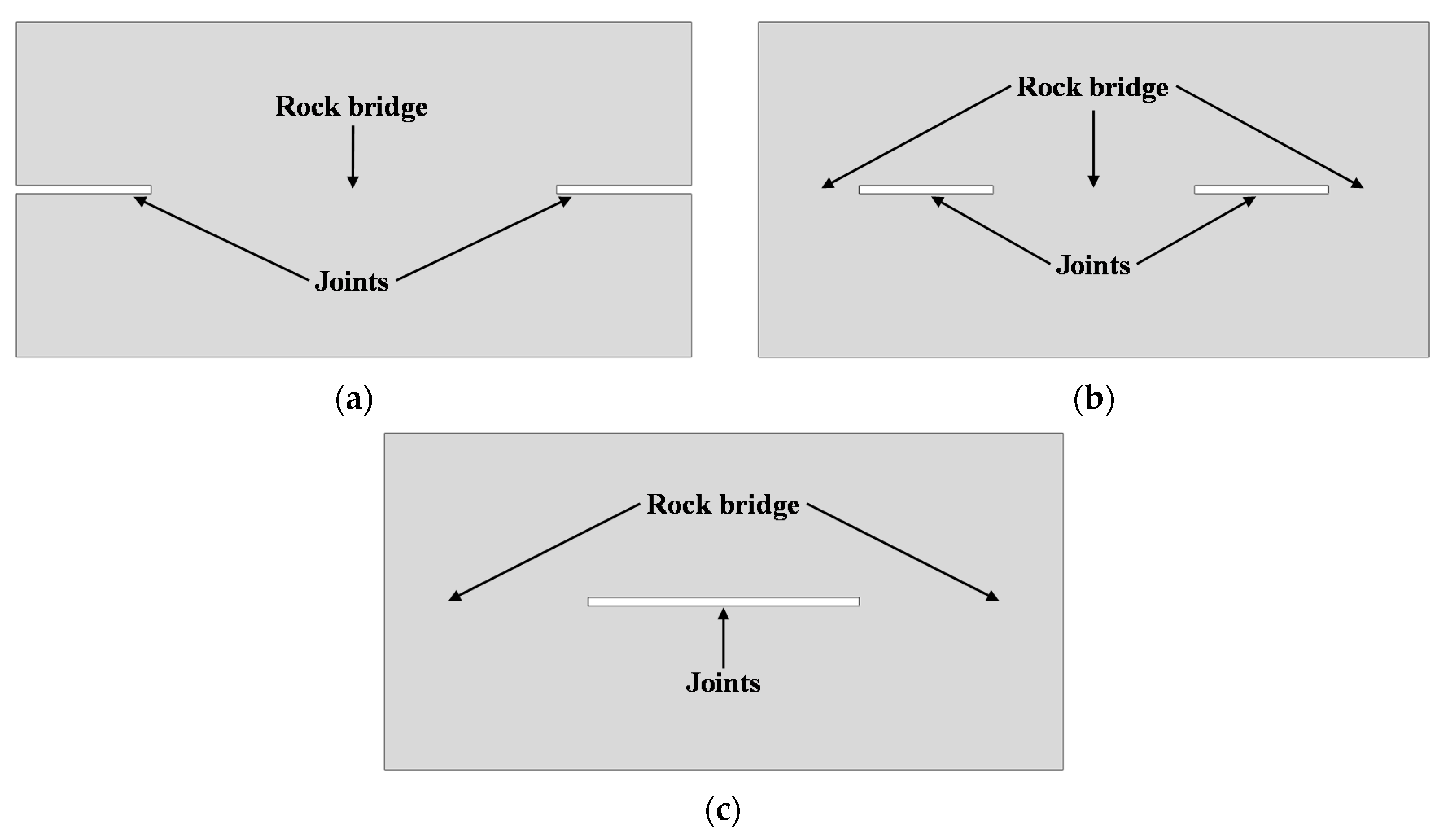
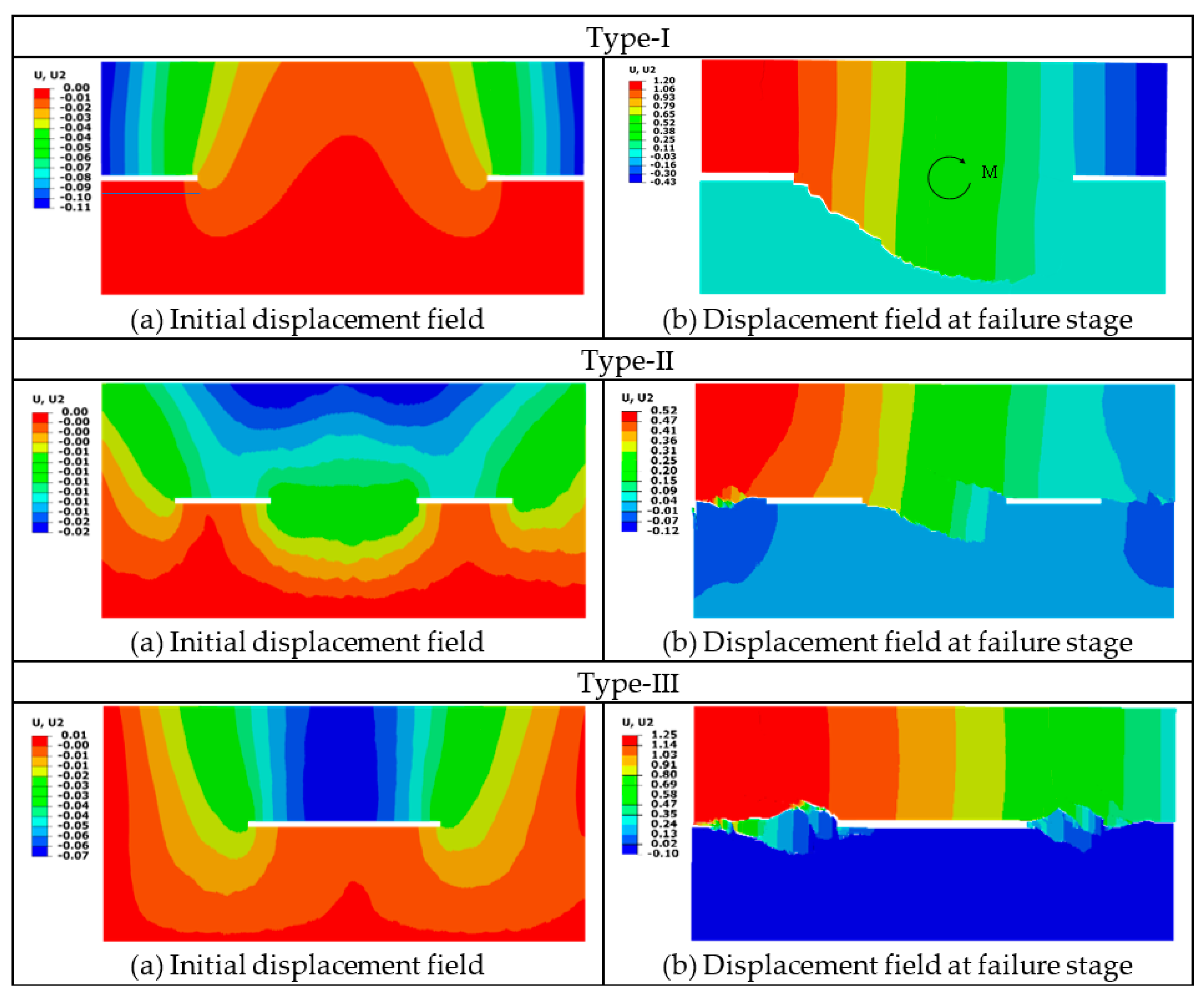
Under the same conditions, the specimen in the type-I is more likely to produce an unbalanced moment around the centroid of the specimen, which causes the opposite ends of the specimen to produce vertical displacements in opposite directions. Due to the strengthening effect of the rock bridge, the vertical displacement on the side away from the loading site is smaller, and as a result, the overall displacement field of the specimen is not simply center-symmetric. At the same time, the distribution of rock bridges in type-II is more dispersed, providing more reinforcement for the joints, and the specimens are subjected to lower dilatancy.

(3)

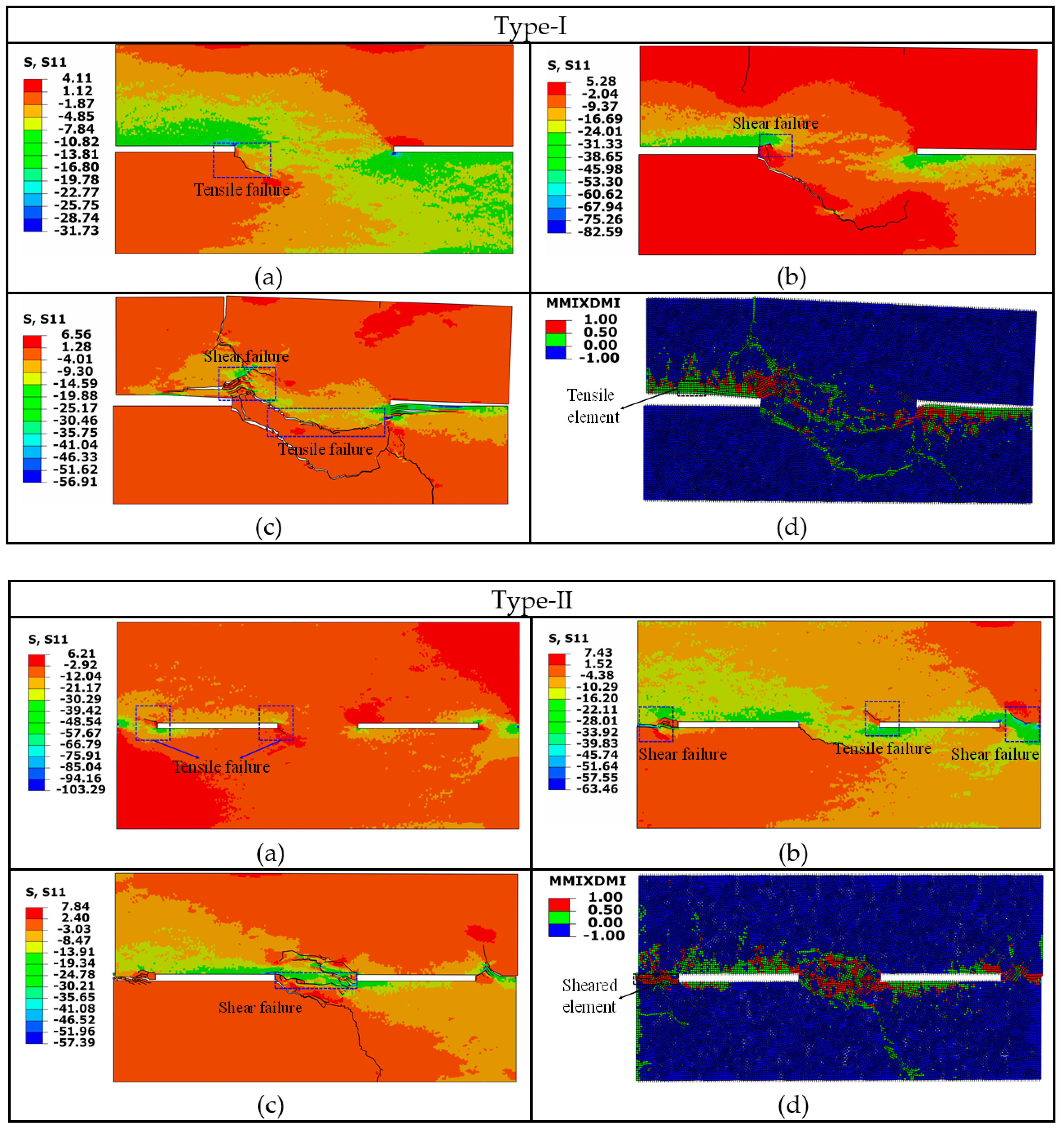
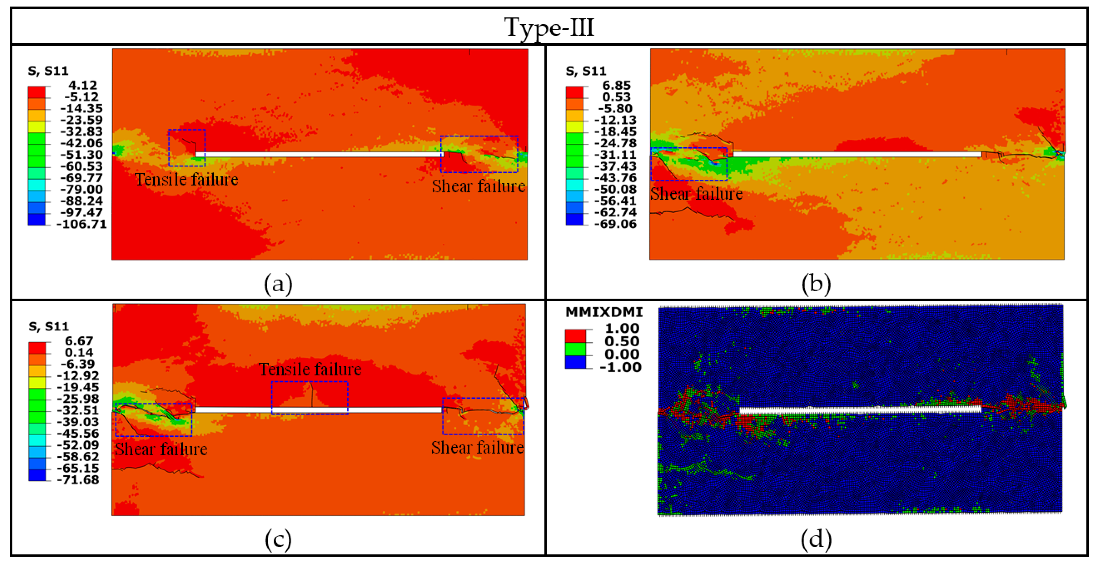
The crack propagation process can be divided into three stages: crack initiation stage, crack evolution stage, and final failure stage. Under the load, the joint tips are prone to stress concentration, where the cohesive elements accumulate more fracture energy and reach the damage evolution stage faster. Initial cracks always start from the joint ends. Affected by the unbalanced moment, more tensile cracks are generated in type-I, while the type-II and type-III penetrated cracks are all shear cracks, and the cracks mainly propagate along the rock bridge.

References

1. Singh, H.K.; Basu, A. A comparison between the shear behavior of ‘real’ natural rock discontinuities and their replicas. Rock Mech. Rock Eng. 2018, 51, 329–340. [Google Scholar] [CrossRef]
2. Niktabar, S.M.; Rao, K.S.; Seshagiri, R.; Shrivastava, A.K. Effect of rock joint roughness on its cyclic shear behavior. J. Rock Mech. Geotech. Eng. 2017, 9, 1071–1084. [Google Scholar] [CrossRef]
3. Li, L.; Chen, D.; Li, S.; Shi, S.; Zhang, M. Numerical analysis and fluid-solid coupling model test of filling-type fracture water inrush and mud gush. Geomech. Eng. 2017, 13, 1011–1025. [Google Scholar]
4. Wang, G.; Han, W.; Jiang, Y.; Luan, H.; Wang, K. Coupling analysis for rock mass supported with CMC or CFC rockbolts based on viscoelastic method. Rock Mech. Rock Eng. 2019, 52, 4565–4588. [Google Scholar] [CrossRef]
5. Li, L.; Sun, S.; Wang, J.; Yang, W.; Fang, Z. Experimental study of the precursor information of the water inrush in shield tunnels due to the proximity of a water-filled cave. Int. J. Rock Mech. Min. Sci. 2020, 130, 104320. [Google Scholar] [CrossRef]
6. Lin, H.; Ding, X.; Yong, R.; Xu, W. Effect of discontinuous joints distribution on shear behavior. C. R. Mec. 2019, 347, 477–489. [Google Scholar] [CrossRef]
7. Chang, L.; Konietzky, H.; Frühwirt, T. Strength Anisotropy of Rock with Crossing Joints: Results of Physical and Numerical Modeling with Gypsum Models. Rock Mech. Rock Eng. 2019, 52, 2293–2317. [Google Scholar] [CrossRef]
8. Guo, S.; Zhou, W.S.; Li, Y.; Jian, C. DDARF analysis on shear tests of jointed rock mass. Appl. Mech. Mate. 2013, 353, 507–510. [Google Scholar] [CrossRef]
9. Yang, J.; Rong, G.; Cheng, L.; Hou, D.; Peng, J. Experimental study on peak shear strength of rock joints. Rock Mech. Rock Eng. 2015, 49, 821–835. [Google Scholar] [CrossRef]
10. Bahrani, N.; Peter, K.; Valley, B. Distinct element method simulation of an analogue for a highly interlocked, non-persistently jointed rockmass. Int. J. Rock Mech. Min. Sci. 2014, 71, 117–130. [Google Scholar] [CrossRef] [Green Version]
11. Pariseau, W.G.; Puri, S.; Schmelter, S.C. A new model for effects of impersistent joint sets on rock slope stability. Int. J. Rock Mech. Min. Sci. 2008, 45, 122–131. [Google Scholar] [CrossRef]
12. Lajtai, E.Z. Shear strength of weakness planes in rock. Int. J. Rock Mech. Min. Sci. Geomech. Abs. 1969, 6, 499–515. [Google Scholar] [CrossRef]
13. Stimpson, B. Failure of slopes containing discontinuous planar points. In 19th U.S. Symposium on Rock Mechanics (USRMS); American Rock Mechanics Association: Reno, NE, USA, 1978. [Google Scholar]
14. Yang, X.; Qiao, W. Numerical investigation of the shear behavior of granite materials containing discontinuous joints by utilizing the flat-joint model. Comput. Geotech. 2018, 104, 69–80. [Google Scholar] [CrossRef]
15. Lisjak, A.; Grasselli, G. A review of discrete modeling techniques for fracturing processes in discontinuous rock masses. J. Rock Mech. Geotech. Eng. 2014, 6, 301–314. [Google Scholar] [CrossRef] [Green Version]
16. Han, W.; Li, G.; Sun, Z.; Luan, H. Numerical investigation of a foundation pit supported by a composite soil nailing structure. Symmetry 2020, 12, 252. [Google Scholar] [CrossRef] [Green Version]
17. Wang, C.; Jiang, Y.; Liu, R.; Wang, C.; Zhang, Z.; Sugimoto, S. Experimental Study of the Nonlinear Flow Characteristics of Fluid in 3D Rough-Walled Fractures During Shear Process. Rock Mech. Rock Eng. 2020, 53, 2581–2604. [Google Scholar] [CrossRef]
18. Jing, L.; Hudson, J.A. Numerical methods in rock mechanics. Int. J. Rock Mech. Min. Sci. 2002, 39, 409–427. [Google Scholar] [CrossRef]
19. Li, L.; Sun, S.; Wang, J. Development of compound EPB shield model test system for studying the water inrushes in karst regions. Tunn. Undergr. Space Technol. 2020, 101, 103404. [Google Scholar] [CrossRef]
20. Song, S.; Li, S.; Li, L. Model test study on vibration blasting of large cross-section tunnel with small clearance in horizontal stratified surrounding rock. Tunn. Undergr. Space Technol. 2019, 92, 103013. [Google Scholar] [CrossRef]
21. Potyondy, D.O.; Cundall, P.A.; Lee, C.A. Modelling rock using bonded assemblies of circular particles. In 2nd North American Rock Mechanics Symposium; American Rock Mechanics Association: Montreal, QC, Cananda, 1996. [Google Scholar]
22. Potyondy, D.O.; Cundall, P.A. A bonded-particle model for rock. Int. J. Rock Mech. Min. Sci. 2004, 41, 1329–1364. [Google Scholar] [CrossRef]
23. Hazzard, J.F.; Collins, D.S.; Pettitt, W.S.; Young, R.P. Simulation of unstable fault slip in granite using a bonded-particle model. Pure Appl. Geophys. 2002, 159, 221–245. [Google Scholar] [CrossRef]
24. Wang, X.; Yuan, W.; Yan, Y.; Zhang, X. Scale effect of mechanical properties of jointed rock mass: A numerical study based on particle flow code. Geomech. Eng. 2020, 21, 259–268. [Google Scholar]
25. Zhang, Y.; Wang, G.; Jiang, Y.; Wang, S.; Zhao, H.; Jing, W. Acoustic emission characteristics and failure mechanism of fractured rock under different loading rates. Shock. Vib. 2017, 2017, 5387459. [Google Scholar] [CrossRef] [Green Version]
26. Zhao, Z. Gouge particle evolution in a rock fracture undergoing shear: A microscopic DEM study. Rock Mech. Rock Eng. 2013, 46, 1461–1479. [Google Scholar] [CrossRef]
27. Liu, S.Y. Simulation of high-speed scratching process of marble based on finite element/discrete element coupling method. Diam. Abr. Eng. 2019, 1, 18. [Google Scholar]
28. Cho, S.H.; Ogata, Y.; Kaneko, K. Strain-rate dependency of the dynamic tensile strength of rock. Int. J. Rock Mech. Min. Sci. 2003, 40, 763–777. [Google Scholar] [CrossRef]
29. Dong, S.; Wang, Y.; Xia, Y. A finite element analysis for using brazilian disk in split hopkinson pressure bar to investigate dynamic fracture behavior of brittle polymer materials. Polym. Test. 2006, 25, 943–952. [Google Scholar] [CrossRef]
30. Hao, Y.; Hao, H. Finite element modelling of mesoscale concrete material in dynamic splitting test. Adv. Struct. Eng. 2016, 19, 1027–1039. [Google Scholar] [CrossRef]
31. Wu, Z.; Cui, W.; Fan, L.; Liu, Q. Mesomechanism of the dynamic tensile fracture and fragmentation behaviour of concrete with heterogeneous mesostructured. Constr. Build. Mater. 2019, 217, 573–591. [Google Scholar] [CrossRef]
32. Zhou, X.P.; Yang, H.Q. Multiscale numerical modeling of evolution and coalescence of multiple cracks in rock masses. Int. J. Rock Mech. Min. Sci. 2012, 55, 15–27. [Google Scholar] [CrossRef]
33. Khosravani, M.R.; Silani, M.; Weinberg, K. Fracture studies of ultra-high performance concrete using dynamic Brazilian tests. Theor. Appl. Fract. Mech. 2018, 93, 302–310. [Google Scholar] [CrossRef]
34. Strouboulis, T.; Copps, K.; Ka, I.B. The generalized finite element method: An example of its implementation and illustration of its performance. Int. J. Numer. Methods Eng. 2000, 47, 1401–1417. [Google Scholar] [CrossRef]
35. Fan, L.F.; Wu, Z.J.; Wan, Z.; Gao, J.W. Experimental investigation of thermal effects on dynamic behavior of granite. Appl. Therm. Eng. 2017, 125, 94–103. [Google Scholar] [CrossRef]
36. Munjiza, A. The Combined Finite-Discrete Element Method; John Wiley & Sons: Hoboken, NJ, USA, 2004. [Google Scholar] [CrossRef]
37. Lisjak, A.; Figi, D.; Grasselli, G. Fracture development around deep underground excavations: Insights from FDEM modelling. J. Rock Mech. Geol. Eng. 2014, 6, 493–505. [Google Scholar] [CrossRef] [Green Version]
38. Lisjak, A.; Garitte, B.; Grasselli, G.; Muller, H.; Vietor, T. The excavation of a circular tunnel in a bedded argillaceous rock (Opalinus Clay): Short-term rock mass response and FDEM numerical analysis. Tunn. Undergr. Space. Technol. 2015, 45, 227–248. [Google Scholar] [CrossRef] [Green Version]
39. Tatone, B.; Lisjak, A.; Mahabadi, O.; Vlachopoulos, N. Incorporating Rock Reinforcement Elements into Numerical Analyses Based on the Hybrid Finite-Discrete Element Method (FDEM); International Society of Rock Mechanics: Montreal, QC, Cananda, 2015. [Google Scholar] [CrossRef]
40. Mahabadi, O.; Lisjak, A. Application of FEMDEM to analyze fractured rock masses. Int. Dis. Frac. Network. Eng. Conf. 2014. [Google Scholar] [CrossRef]
41. Dugdale, D.S. Yielding of steel sheets containing slits. J. Mech. Phys. Solids 1960, 8, 100–104. [Google Scholar] [CrossRef]
42. Barenblatt, G.I. The mechanical theory of equilibrium cracks in brittle fracture. Adv. Appl. Mech. 1962, 7, 55–129. [Google Scholar]
43. Su, X.T.; Yang, Z.; Liu, G. Monte Carlo simulation of complex cohesive fracture in random heterogeneous quasi-brittle materials. Int. J. Sol. Struct. 2009, 46, 3222–3234. [Google Scholar]
44. Jiang, H.; Meng, D. 3D numerical modelling of rock fracture with a hybrid finite and cohesive element method. Eng. Fract. Mech. 2018, 199, 280–293. [Google Scholar] [CrossRef]
45. Chang, X.; Guo, T.; Zhang, S. Cracking behaviours of layered specimen with an interface crack in Brazilian tests. Eng. Fract. Mech. 2020, 228, 106904. [Google Scholar] [CrossRef]
46. Haddad, M.; Sepehrnoori, K. XFEM-Based CZM for the Simulation of 3D Multiple-Stage Hydraulic Fracturing in Quasi-Brittle Shale Formations. Rock Mech. Rock Eng. 2016, 49, 4731–4748. [Google Scholar] [CrossRef]
47. Zhang, S.; Wang, G.; Jiang, Y. Study on Shear Mechanism of Bolted Jointed Rocks: Experiments and CZM-Based FEM Simulations. Appl. Sci. 2019, 10, 62. [Google Scholar] [CrossRef] [Green Version]
48. Han, W.; Jiang, Y.; Luan, H.; Du, Y.; Zhu, Y.; Liu, J. Numerical investigation on the shear behavior of rock-like materials containing fissure-holes with FEM-CZM method. Comput. Geotech. 2020, 125, 103670. [Google Scholar] [CrossRef]
49. Park, K.; Paulino, G.H. Cohesive zone models: A critical review of traction-separation relationships across fracture surfaces. Appl. Mech. Rev. 2011, 64, 060802. [Google Scholar] [CrossRef]
50. Cong, Y. Experimental study on shear strength of concrete. Concrete 2015, 5, 40–45. [Google Scholar]
51. Alfano, G. On the influence of the shape of the interface law on the application of cohesive-zone models. Compos. Sci. Technol. 2006, 66, 723–730. [Google Scholar] [CrossRef]
52. Du, Y.; Li, T.; Li, W.; Ren, Y. Experimental study of mechanical and permeability behaviors during the failure of sandstone containing two preexisting fissures under triaxial compression. Rock Mech. Rock Eng. 2020, 53, 3673–3697. [Google Scholar] [CrossRef]
53. Basu, A.; Mishra, D.A.; Roychowdhury, K. Rock failure modes under uniaxial compression, brazilian, and point load tests. Bull. Eng. Geol. Environ. 2013, 72, 457–475. [Google Scholar] [CrossRef]
Figure 1. Separation-Traction (S-T) model: (a) mixed-mode cohesive traction response, and (b) constitutive Model of S-T model.
Symmetry 12 01314 g001
Figure 2. Insertion process of cohesive elements: (a) continuous solid elements, (b) split solid elements, (c) re-number nodes, and (d) insert a cohesive element.
Symmetry 12 01314 g002
Figure 3. The uniaxial compression test: (a) uniaxial compression experiment, and (b) numerical model and failure pattern.
Symmetry 12 01314 g003
Figure 4. Uniaxial compression experiment and simulation results.
Symmetry 12 01314 g004
Figure 5. Numerical model of the Brazilian test: (a) numerical simulation model, (b) failure pattern, and (c) experimental results.
Symmetry 12 01314 g005
Figure 6. The Brazilian test and simulation results.
Symmetry 12 01314 g006
Figure 7. Symmetrical calculation model used in this paper. σ : Normal stress, τ : Shear stress, L j : Joint length, L r : Rock bridge length, H : Model width, L : Model length, e j : Joint aperture.
Symmetry 12 01314 g007
Figure 8. Symmetrical three types of joint distribution: (a) Type-I: both sided, (b) Type-II: scattered, and (c) Type-III: central.
Symmetry 12 01314 g008
Figure 9. Stress-strain curve at the persistence of 0.2: (a) Type-I, (b) Type-II, (c) Type-III.
Symmetry 12 01314 g009
Figure 10. Peak strength and decrease value: (a) peak strength and (b) decrease value.
Symmetry 12 01314 g010
Figure 11. The vertical displacement field of specimens: (a) initial displacement field and (b) displacement field at failure stage.
Symmetry 12 01314 g011
Figure 12. Stress-strain curve at normal stress of 1.0 MPa: (a) Type-I, (b) Type-II, (c) Type-III, and (d) peak stress.
Symmetry 12 01314 g012
Figure 13. Relationship of the peak shear strength of the specimens with joints’ persistence and normal stress.
Symmetry 12 01314 g013
Figure 14. Crack evolution process: (a) crack initiation stage, (b) crack evolution stage, (c) final failure stage, and (d) failure form of cohesive elements.
Symmetry 12 01314 g014aSymmetry 12 01314 g014b
Figure 15. Stress concentration: (a) stress concentration at joint ends, and (b) accumulation of fracture energy.
Symmetry 12 01314 g015