The Response of Nanobeams with Temperature-Dependent Properties Using State-Space Method via Modified Couple Stress Theory

Abstract

At present, with the development in nanotechnology, nanostructures with temperature-dependent properties have been used in nano-electromechanical systems (NEMS). Thus, introducing an accurate mathematical model of nanobeams with temperature-dependent properties is a major and important topic for the design of NEMS. This paper aims to discuss nonlocal nanobeams analysis depending on the theories of Euler–Bernoulli and modified couple-stress (MCS). It also is assumed that the thermal conductivity of the nanobeam is dependent on the temperature. Physical fields of the nanobeam are obtained utilizing Laplace transform and state-space techniques. The effects of the size and nonlocal parameters, variability of thermal conductivity and couple stress on various distributions are presented graphically and studied in detail. Numerical results are presented as application scales and the design of nanoparticles, nanoscale oscillators, atomic force microscopes, and nanogenerators, in which nanoparticles as nanobeams act as essential and basic elements.

1. Introduction

The coupled thermoelasticity theory was expressed by Biot [1] to dispense with the contradiction intrinsic in the classical uncoupled model that deformation variations have no influence on the field of temperature. The heat conduction equations for coupled and uncoupled models are of the diffusion kind expecting unlimited speeds of spread for thermal waves inconsistent with physical phenomena. The coupled thermoelasticity theory is connecting with the theory of Lord and Shulman (LS) [2] as well as Green and Lindsay (GL) [3] by including the temperature relaxing up time in the foundational relations.

Nanotechnology is now considered one of the greatest encouraging advanced technologies to be studied. This important modern technology will have major impacts on many sciences such as human health, space, civil structures, defense industries, mechanical devices, and others. Many endeavors have been committed to constructing nanogadgets with superior physical, electromechanical, and chemical properties. From the point of functionality, the nanodevices could generally be categorized as nanowires, nanorods, nanotubes, nanoplates, and nanoshells. Many efforts have been paid to building nanoscale devices with superior electromechanical, physical, and chemical properties. Nanoscale devices can generally be classified as nanowires, nanotubes, nanorods, and nanopanels [4,5,6,7,8,9].

Microscale and nanomechanical resonators (M/NEMS) that have a quick response and also high sensitivity are generally utilized as modulators and sensors. M/NEMS have suitable significant notice lately due to many significant industrial applications. Careful analysis of different consequences of resonator features, for instance, resonant frequencies and quality factors, is vital to designing the component’s high performance. Several authors have studied the process of heat transfer and the behavior of vibrations of microbeams [10,11,12,13,14,15,16,17,18,19,20,21].

The nonlocal microbeam models got increasing regard in the previous few years. In 1972, Eringen [22,23] has proposed the idea of nonlocal continuum mechanics to deal with problems of small-scale structural materials. Eringen and Edelen [24] constructed a constitutive relation to the nonlocal stress at any point in an integral form depending on the complete assumption that the stress at any point is a function of the strains at the same point. The presented nonlocal theory depends on the strengths amongst atoms and the inside length scale, which are taken into consideration in the constitutive equations like a material parameter. The nonlocal principle of elasticity has been used to investigate the applications inclusive of lattice dispersion of elastic waves, nanomechanics, wave spread in composites, fracture mechanics, surface strain fluids, and decoupling mechanics [25].

Recently, some contradictory results and some inconsistencies in the non-local elasticity approaches have been observed through some recent studies. These observations and paradoxical results have motivated researchers in this field to discuss and deal with these contradictory results. It has been shown through studies in this field that these non-local paradoxes can appear when comparing the results of models based on non-local differentials under different loading boundary conditions. Recently, Romano et al. [26] have introduced some new concepts, including the concept of constitutive boundary conditions, and through the study, they demonstrated that achieving these boundary conditions is a necessary condition for non-local beam models. In order to address the shortcomings of the previous theory and overcome these paradoxes, many studies have been presented and many efforts were made [27,28,29,30,31].

State-space strategies are the basis of the novel theory of control. The important advantage of state-space techniques is the characterization of approaches of importance through differential equations in favoring transport functions. This may appear to be a return to the previous primitive period where the differential equations likewise formed a way to represent the method of dynamic operations. However, in the previous duration, the processes were easy and sufficient to them with only one differential equation for a reasonably low order. The potential function technique is frequently employed to solve some problems of thermoelasticity theory. However, this has various shortcomings as described in [32,33].

Sherief and Anwar [34] treated a generalized thermoelastic problem based on LS theory without heat sources. Additionally, Zenkour and Abouelregal [35] investigated the response of nanobeams of temperature-dependent thermal conductivity subjected to sine wave heating.

The size effect can be circumvented by higher-order continuum theories. In this study, Euler–Bernoulli microbeams are analyzed with modified strain gradient theory (MSGT) and modified couple stress theory (MCST). A few models are considered for small scale and nanostructures, including strain gradient and couple stress models. The modified couple-stress (MCS) theory can be observed as an exceptional instance of the strain gradient model [36]. The MCS theory considers the revolutions as a variable to delineate curvature, while the strain inclination model considers the strains as a variable to pronounce curvature. Different investigations about these theories have been available in the scientific literatures [37,38,39,40,41,42].

Micromorphic mechanics is currently a very active field of research both from theoretical and applied perspectives. Therefore, it is possible to reflect on concerning the foundations of the current state of the art and checking the requirements of essential mechanical well-posedness. Romano et al. [43] investigated the kinematics of generalized continuity and made the main points regarding the definition of a tangential strain measure in general. Barbagallo et al. [44] and Neff et al. [45] studied the anisotropic classes of the fourth-tiered elastic tensors of the relaxed micromorphic model and also introducing their second-order counterpart Voigt-type vector notation.

In the present paper we introduce a generalized thermoelastic model for nanobeams when thermal conductivity is variable depending on the model of nonlocal elasticity and thermoelasticity. The technique of Laplace transform can be applied to get the distributions of the displacement, temperature, deflection, and the stress of the nanobeam. The influences of nonlocal parameter (size effect), the thermal conductivity variation, and the term of the modified couple-stress model will be considered and represented graphically. In addition, numerical results for different boundary conditions, different engineering parameters, and non-local parameter values are presented to explain in detail the effects of each of them on different fields of the nanobeam.

2. Mathematical Modeling for Nonlocal Beam Theory

Despite previous studies in the non-local field, it has also been proven that the fully non-local constitutive laws and the local/non-local mixture represent the same non-local constitutive model, but with different degrees of singularity. Additionally, some results demonstrated that the ill-posedness of Eringen’s could not be eliminated since homogeneous parts of the non-local fields could not be formed correctly using the non-local constitutive model.

In this paper, we used the theory of nonlocal elasticity, proposed by Eringen [22,23,24]. In this model, the constitutive relations can be written as

$${\sigma }_{kl}-\xi {\nabla }^2{\sigma }_{kl}={\tau }_{kl},$$

(1)

where ${\sigma }_{kl}$ and ${\tau }_{kl}$ are respectively, nonlocal and stress tensors, ${\nabla }^2$ is the Laplacian operator, and $\xi ={\left(e_{0}a\right)}^2$ is the small scale coefficient. The parameter $a$ is the interior characteristic length and $e_0$ is a constant suitable to each material and obtained by experiment. We can also note that when the parameter $a$ is ignored $\left(\xi =0\right)$ Equation (1) reduces to constitutive equations in elasticity theory.

The stress–strain–temperature relations can be written as

$${\tau }_{kl}=\lambda {\epsilon }_{mm}{\delta }_{kl}+\mu {\epsilon }_{kl}-\gamma {\delta }_{kl}\theta$$

(2)

where $\theta =T-T_0$ is the of temperature, $T$ is the temperature distribution and $T_0$ is the environmental temperature, ${\epsilon }_{kl}$ are the classical Cauchy relations at a point $x^{\prime }$ in the body, $\lambda$ and $\mu$ are the Lamé’s constants, $\gamma ={\alpha }_t\left(3\lambda +2\mu \right)=E{\alpha }_t/\left(1-2\nu \right)$, ${\alpha }_t$ is the coefficient of thermal expansion, $E$ denotes the Young’s modulus, $\nu$ being the Poisson’s ratio, and ${\delta }_{kl}$ is the Kronecker delta function. The Lamé constants $\lambda$ and $\mu$ can be expressed as $\lambda =E\nu /\left(1+\nu \right)\left(1-2\nu \right)$ and $\mu =E/2\left(1+\nu \right)$.

The classical Cauchy relations are given by

$$2{\epsilon }_{kl}=\frac{\partial u_k}{\partial x_l}+\frac{\partial u_l}{\partial x_k}$$

(3)

where $u_k$ are the displacement vector components.

Based on the MSC theory, the $m_{kl}$ deviatoric part of the couple stress (CS) tensor and ${\chi }_{kl}$ the homogeneous part of the curvature tensor satisfy the relations [46,47]:

$$m_{kl}=2l^2\mu {\chi }_{kl}=2\alpha {\chi }_{kl}$$

(4)

$$2{\chi }_{kl}=\frac{\partial {\omega }_k}{\partial x_l}+\frac{\partial {\omega }_l}{\partial x_k}$$

(5)

where $l$ denotes the length scale parameter and ${\omega }_k$ is the rotation vector, which is given by [47]:

$$2{\omega }_k={\epsilon }_{kji}{u}_{i,j}.$$

(6)

The generalized Fourier law supplanted by the Maxwell-Cattaneo can be written as

$$\left(1+{\tau }_0\frac{\partial }{\partial t}\right)\mathit{q}=-\nabla \left(K\left(\theta \right)\theta \left(x,t\right)\right),$$

(7)

where $\mathit{q}$ is the vector of the heat flux, $K\left(\theta \right)$ denotes the temperature-dependent thermal conductivity, and ${\tau }_0$ is the relaxation time. Based on Equation (7), the generalized heat conduction corresponding to LS model can be expressed as [2]

$${\left(K{\theta }_{,i}\right)}_{,i}+\left(1+{\tau }_0\frac{\partial }{\partial t}\right)\left(\rho Q\right)=\left(1+{\tau }_0\frac{\partial }{\partial t}\right)\left(\rho C_E\left(\theta \right)\frac{\partial \theta }{\partial t}+\gamma T_0\frac{\partial e}{\partial t}\right).$$

(8)

where $C_E\left(\theta \right)$ is the temperature-dependent specific heat, $Q$ is the heat source, and $e={\epsilon }_{mm}$ is the volumetric strain.

3. Formulation of the Problem

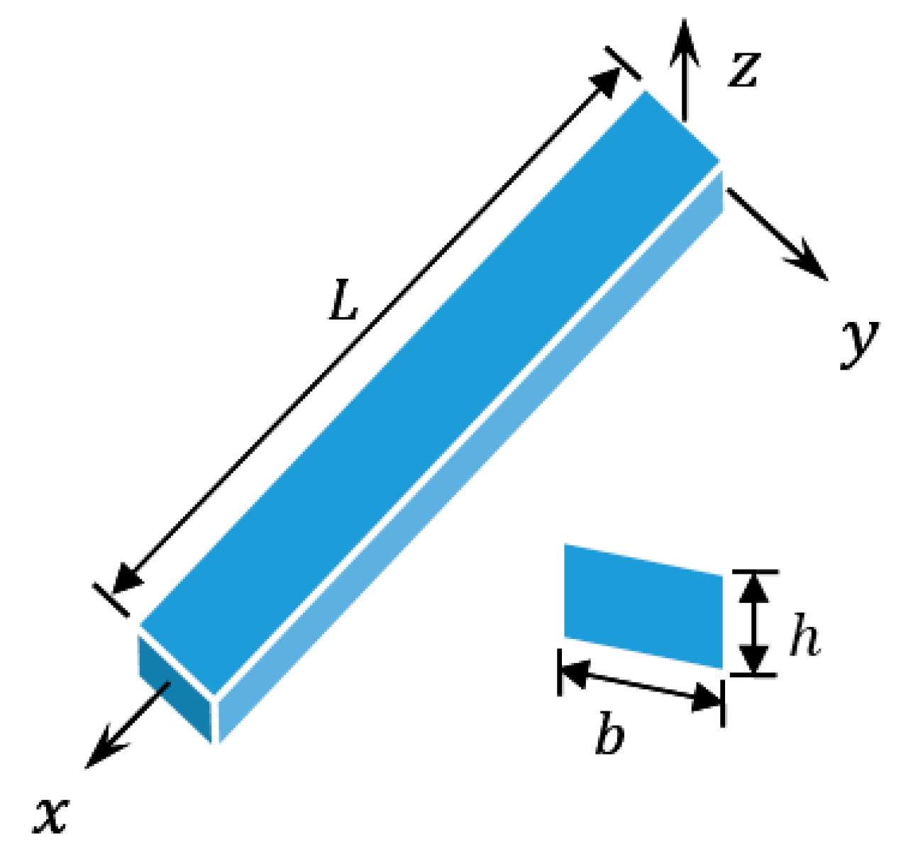
Figure 1 illustrates a thermoelastic Euler–Bernoulli nanobeam isotropic nanobeam. As shown in the Figure the nanobeam has the length $\left(0\le x\le L\right)$, width $b$ $\left(-b/2\le y\le b/2\right)$, thickness $h$ $\left(-h/2\le z\le h/2\right)$, Young’s modulus $E,$ and cross-sectional area $A$. Upon the Euler–Bernoulli beams model and considering that the problem is one-dimensional, the displacement field and the axial strain of the beam can be presented as [47]

$$u=-z\frac{\partial w}{\partial x},\hspace{1em}v=0,\hspace{1em}w=w\left(x,t\right),\hspace{1em}{\epsilon }_{xx}=-z\frac{{\partial }^{2}w}{\partial x^2},$$

(9)

where $w$ is the lateral deflection (displacement in the $z$ direction).

The components of rotation vector are expressed as:

$${\omega }_y=-\frac{\partial w}{\partial x}, {\omega }_x={\omega }_z=0$$

(10)

Additionally, putting Equation (10) in Equation (5), we obtained the curvature tensor components as:

$$2{\chi }_{xy}=-\frac{{\partial }^{2}w}{\partial x^2}, {\chi }_{xz}={\chi }_{zx}={\chi }_{zy}={\chi }_{yz}=0.$$

(11)

Considering conditions of the plane stress, the local constitutive relations along the $x$-axis has only the nonzero components

$${\tau }_{xx}=-E\left(z\frac{{\partial }^{2}w}{\partial x^2}+{\alpha }_T\theta \right),m_{xy}=-l^2\mu \frac{{\partial }^{2}w}{\partial x^2}$$

(12)

As indicated by Eringen theory [22], the constitutive equations (nonlocal) can be presented as:

$${\sigma }_x-\xi \frac{{\partial }^2{\sigma }_x}{\partial x^2}={\tau }_{xx}=-E\left(z\frac{{\partial }^{2}w}{\partial x^2}+{\alpha }_T\theta \right),$$

(13)

$${\mu }_{xy}-\xi \frac{{\partial }^2{\mu }_{xy}}{\partial x^2}=m_{xy}=-l^2\mu \frac{{\partial }^{2}w}{\partial x^2}$$

(14)

where ${\mu }_{xy}$ is the nonlocal couple stress and ${\alpha }_T={\alpha }_t/\left(1-2\nu \right)$.

The motion equation for transverse vibration of nanobeams can be rewritten as

$$\frac{\partial V\left(x,t\right)}{\partial x}=\rho A\frac{{\partial }^{2}w}{\partial t^2}$$

(15)

$$V\left(x,t\right)=\frac{\partial M\left(x,t\right)}{\partial x}$$

(16)

where $V\left(x,t\right)$ is the resultant shear force and $M\left(x,t\right)$ is bending moment of the nanobeam.

From Equations (15) and (16), we get:

$$\frac{{\partial }^{2}M}{\partial x^2}=\rho A\frac{{\partial }^{2}w}{\partial t^2}.$$

(17)

Depending on the MCS model and Euler–Bernoulli nanobeam theories, the stress $M_m$ and couple stress $M_{\sigma }$ resultants can be presented as [46,47]

$$\begin{array}{c}{M}_{\sigma }=b{{\displaystyle \int }}_{-h/2}^{h/2}z{\sigma }_x\mathrm{d}z,\\ M_m=b{{\displaystyle \int }}_{-h/2}^{h/2}{\mu }_{xy}\mathrm{d}z.\end{array}$$

(18)

The total resultant nonlocal bending moment $M$ of the nanobeam on the $x$ direction can be calculated using the relation [47]:

$$M=M_{\sigma }+M_m$$

(19)

If the thermal moment $M_T$ is defined as

$$M_T=\frac{12}{h^3}{\int }_{-h/2}^{h/2}\theta \left(x,z,t\right)z\mathrm{d}z,$$

(20)

then the equation of bending moment $M$ given in Equation (19) after using Equations (13), (14), and (18) reduces to

$$M\left(x,t\right)-\xi \frac{{\partial }^{2}M\left(x,t\right)}{\partial x^2}=-EI\left(\frac{{\partial }^{2}w}{\partial x^2}+{\alpha }_T{M}_T\right)-l^2\mu A \frac{{\partial }^{2}w}{\partial x^2},$$

(21)

where $I=b{h}^3/12$ and $EI$ are respectively, the inertia moment of the cross-section and the flexural rigidity.

By substituting Equation (21) into Equation (17), motion Equation (17) can be rewritten in the form

$$\left[\left(1+\frac{6l^2}{h^2\left(1+\nu \right)}\right)\frac{{\partial }^4}{\partial x^4}+\frac{\rho A}{EI}\frac{{\partial }^2}{\partial t^2}\left(1-\xi \frac{{\partial }^2}{\partial x^2}\right)\right]w+{\alpha }_T\frac{{\partial }^2{M}_T}{\partial x^2}=0.$$

(22)

Additionally, substituting Equation (17) into Equation (21) we have:

$$M\left(x,t\right)=\xi \rho A\frac{{\partial }^{2}w}{\partial t^2}-EI\left((1+\frac{6l^2}{h^2\left(1+\nu \right)})\frac{{\partial }^{2}w}{\partial x^2}+{\alpha }_T{M}_T\right).$$

(23)

Using Equation (9), the generalized non-Fourier equation of heat conduction (8) in under LS model [2] can be given as

$$\frac{\partial }{\partial x}\left(K\left(\theta \right)\frac{\partial \theta }{\partial x}\right)+\frac{\partial }{\partial z}\left(K\left(\theta \right)\frac{\partial \theta }{\partial z}\right)=\left(1+{\tau }_0\frac{\partial }{\partial t}\right)\left(\rho C_E\left(\theta \right)\frac{\partial \theta }{\partial t}-\gamma T_{0}z\frac{\partial }{\partial t}\left(\frac{{\partial }^{2}w}{\partial x^2}\right)\right)$$

(24)

In applied engineering problems, the thermal conductivity coefficient depends on the heat in that the numerical estimation of thermal conductivity changes with temperature. Therefore, the equation of heat conduction in this case is a nonlinear equation. The determination of the thermal conductivity is important in numerous thermal management frameworks. Particularly, an exact forecast of the thermal conductivity is important to attain an ideal thermal governor system [48].

One of our objectives in this paper was to explain the effect of the temperature dependency of thermal conductivity, taking into consideration that the other of the parameters are constant. We assumed that thermoelastic materials have temperature-dependent properties on the formula (Zhang [48])

$$\rho C_E\left(\theta \right)=\frac{K\left(\theta \right)}{k}$$

(25)

where $k$ is the thermal diffusivity. Introducing Equation (25) into Equation (24), the conduction equation can be rewritten as

$$\frac{\partial }{\partial x}\left(K\left(\theta \right)\frac{\partial \theta }{\partial x}\right)+\frac{\partial }{\partial z}\left(K\left(\theta \right)\frac{\partial \theta }{\partial z}\right)=\left(1+{\tau }_0\frac{\partial }{\partial t}\right)\left(\frac{K\left(\theta \right)}{k}\frac{\partial \theta }{\partial t}-\gamma T_{0}z\frac{\partial }{\partial t}\left(\frac{{\partial }^{2}w}{\partial x^2}\right)\right).$$

(26)

4. Analytical Solution

Considering the following mapping (Kirchhoff’s transform), which to convert the nonlinear terms of the temperature to be linear, we considered the following mapping [35]:

$$\phi =\frac{1}{K_0}{{\displaystyle \int }}_0^{\theta }K\left(\vartheta \right)\mathrm{d}\vartheta ,$$

(27)

where $K_0$ denotes the temperature-independent thermal conductivity. With the utility of Equation (26), Equation (30) is reduced to the linear partial differential equation

$$\left(\frac{{\partial }^2}{\partial x^2}+\frac{{\partial }^2}{\partial z^2}\right)\phi =\left(1+{\tau }_0\frac{\partial }{\partial t}\right)\left(\frac{1}{k}\frac{\partial \phi }{\partial t}-\frac{\gamma T_0}{K_0}z\frac{\partial }{\partial t}\left(\frac{{\partial }^{2}w}{\partial x^2}\right)\right)$$

(28)

We considered that the top and bottom surfaces of the nanobeam have no heat flow. This means that at $z=\pm h/2$, $\frac{\partial \theta }{\partial z}=\frac{\partial \phi }{\partial z}=0$. Additionally, we assumed that the variation of the functions $\theta \left(x,z,t\right)$ and $\phi \left(x,t,z\right)$ are in a sinusoidal variation during the thickness direction given by

$$\left\{\begin{array}{c}\theta \left(x,z,t\right)\\ \phi \left(x,t,z\right)\end{array}\right\}=\left\{\begin{array}{c}\mathsf{\Theta }\left(x,t\right)\\ \mathsf{\Phi }\left(x,t\right)\end{array}\right\}\sin \left(pz\right), p=\frac{\pi }{h}.$$

(29)

This leads to the following equations

$$M_T=\frac{12}{h^3}{{\displaystyle \int }}_{-h/2}^{h/2}\theta \left(x,z,t\right)z\mathrm{d}z=\frac{24}{{\pi }^{2}h}\mathsf{\Phi }\left(x,t\right)$$

(30)

Using the previous equation we get Equations (22) and (23) as

$$\left[S_1\frac{{\partial }^4}{\partial x^4}+\frac{\rho A}{EI}\frac{{\partial }^2}{\partial t^2}\left(1-\xi \frac{{\partial }^2}{\partial x^2}\right)\right]w+\frac{24{\alpha }_T}{{\pi }^{2}h}\frac{{\partial }^2\mathsf{\Phi }}{\partial x^2}=0.$$

(31)

$$M\left(x,t\right)=\xi \rho A\frac{{\partial }^{2}w}{\partial t^2}-EI\left(S_1\frac{{\partial }^{2}w}{\partial x^2}+\frac{24{\alpha }_T}{{\pi }^{2}h}\frac{{\partial }^2\mathsf{\Phi }}{\partial x^2}\right),$$

(32)

where

$$S_1=\left(1+\frac{6l^2}{h^2\left(1+\nu \right)}\right)$$

Substituting Equation (29) into Equation (28) and integrating with respect to $z$ from $-h/2$ to $-h/2$ and with, we get

$$\frac{{\partial }^2\mathsf{\Phi }}{\partial x^2}-\frac{{\pi }^2}{h^2}\mathsf{\Phi }=\left(1+{\tau }_0\frac{\partial }{\partial t}\right)\frac{\partial }{\partial t}\left(\frac{1}{k}\mathsf{\Phi }-\frac{\gamma T_0{\pi }^{2}h}{24K_0}\frac{{\partial }^{2}w}{\partial x^2}\right).$$

(33)

The following non-dimensional values can be used to convert basic equations in non-dimensional form:

$$\begin{array}{c}\left\{x^{\prime },w^{\prime },u^{\prime },z^{\prime }\right\}=\frac{1}{L}\left\{x,w,u,z\right\}, \left\{t^{\prime },{\tau }_0^{\prime }\right\}=\frac{c}{L}\left\{t,{\tau }_0\right\},{\mathsf{\Theta }}^{\prime }=\frac{\gamma }{E}\mathsf{\Theta },\\ {\mathsf{\Phi }}^{\prime }=\frac{\gamma }{E}\mathsf{\Phi }, {\xi }^{\prime }=L^2\xi , M^{\prime }=\frac{1}{bEI}M, c^2=\frac{E}{\rho }. \end{array}$$

(34)

Consequently, Equations (31)–(33) will be in the form (neglecting the dashes)

$$\left[\frac{{\partial }^4}{\partial x^4}+\frac{{\partial }^2}{\partial t^2}\left(A_1-A_3\frac{{\partial }^2}{\partial x^2}\right)\right]w+A_2\frac{{\partial }^2\mathsf{\Theta }}{\partial x^2}=0,$$

(35)

$$\frac{{\partial }^2\mathsf{\Phi }}{\partial x^2}-A_4\mathsf{\Phi }=\left(1+{\tau }_0\frac{\partial }{\partial t}\right)\frac{\partial }{\partial t}\left(A_6\mathsf{\Phi }-A_5\frac{{\partial }^{2}w}{\partial x^2}\right),$$

(36)

$$M\left(x,t\right)=A_7\frac{{\partial }^{2}w}{\partial t^2}-A_8\frac{{\partial }^{2}w}{\partial x^2}-A_9\mathsf{\Theta }.$$

(37)

The constants $A_i$, ($i=1,2,3,4)$ in Equations (35)–(37) are

$$\begin{array}{c}{A}_1=\frac{12L^2}{S_1{h}^2},\hspace{1em}{A}_2=\frac{24L}{S_1{\pi }^{2}h},\hspace{1em}{A}_3=\xi A_1,\hspace{1em}{A}_4=\frac{L^2{\pi }^2}{h^2},\hspace{1em}{A}_5=\frac{\gamma {\alpha }_T{\pi }^{2}Lh}{24K_0},\hspace{1em}\\ A_6=\frac{cL}{k},\hspace{1em}{A}_7=\frac{\xi }{h{L}^3},\hspace{1em}{A}_8=\frac{hS}{12L},\hspace{1em}{A}_9=\frac{2}{{\pi }^2}\end{array}$$

(38)

Initial conditions are assumed to be homogeneous in the form

$${w\left(x,t\right)|}_{t=0}={\frac{\partial w\left(x,t\right)}{\partial t}|}_{t=0}=0, {\mathsf{\Phi }\left(x,t\right)|}_{t=0}={\frac{\partial \mathsf{\Phi }\left(x,t\right)}{\partial t}|}_{t=0}=0.$$

(39)

The following mechanical boundary conditions are assumed:

$${w\left(x,t\right)|}_{x=0,L}=0, {\frac{{\partial }^{2}w\left(x,t\right)}{\partial x^2}|}_{x=0,L}=0.$$

(40)

Additionally, we assumed that the surface $x=0$ is thermally loaded, i.e.,

$${\mathsf{\Theta }\left(x,t\right)|}_{x=0}=f\left(t\right)={\mathsf{\Theta }}_{0}H\left(t\right),$$

(41)

where ${\mathsf{\Theta }}_0$ is a constant and $H\left(t\right)$ is Heaviside unite step function. Additionally, the thermal conductivity $K\left(\theta \right)$ is considerd to be a linear function of the temperature $\theta$ as [35]

$$K\left(\theta \right)=K{ }_0\left(1+K_1\theta \right), K_1\ge 0.$$

(42)

where the parameters $K_0$ and $K_1$ are constants.

By using the mapping in Equation (17), one gets

$$\phi =\theta +\frac{K_1{\theta }^2}{2}.$$

(43)

Using Equation (41), then one gets

$$\phi \left(0,t\right)={\theta }_0+\frac{K_1{\theta }_0^2}{2}{\left(H\left(t\right)\right)}^2$$

(44)

5. Laplace Transform Technique

To solve the problem, the Laplace transform technique is applied to Equations (35)–(37) to obtain

$$\left[\frac{{\mathrm{d}}^4}{\mathrm{d}{x}^4}-A_3{s}^2\frac{{\mathrm{d}}^2}{\mathrm{d}{x}^2}+A_1{s}^2\right]\overline{w}=-A_2\frac{{\mathrm{d}}^2\overline{\mathsf{\Phi }}}{\mathrm{d}{x}^2},$$

(45)

$$\left(\frac{{\mathrm{d}}^2}{\mathrm{d}{x}^2}-B_1\right)\overline{\mathsf{\Phi }}=-B_2\frac{{\mathrm{d}}^2\overline{w}}{\mathrm{d}{x}^2},$$

(46)

$$\overline{M}\left(x,s\right)=-\left(A_8\frac{{\mathrm{d}}^2}{\mathrm{d}{x}^2}-A_7{s}^2\right)\overline{w}-A_9\overline{\mathsf{\Theta }},$$

(47)

where

$$B_1=A_4+s\left(1+{\tau }_{0}s\right), B_2=s\left(1+{\tau }_{0}s\right)A_5.$$

By introducing a new function $\overline{\psi }$, satisfies the following equation

$$\frac{{\mathrm{d}}^2\overline{w}}{\mathrm{d}{x}^2}=\overline{\psi }.$$

(48)

Substituting the previous equation in Equations (41) and (42), then one obtains

$$\frac{{\mathrm{d}}^2\overline{\mathsf{\Phi }}}{\mathrm{d}{x}^2}=B_1\overline{\mathsf{\Phi }}-B_2\overline{\psi },$$

(49)

$$\frac{{\mathrm{d}}^2\overline{\psi }}{\mathrm{d}{x}^2}=-B_3\overline{w}-B_4\overline{\mathsf{\Phi }}+B_5\overline{\psi },$$

(50)

where

$$B_3=A_{1}s\left(1+{\tau }_{0}s\right), B_4=B_1{A}_2 B_5=s\left(1+{\tau }_{0}s\right)A_3+B_2{A}_2.$$

6. Mathematical Method of State-Space Approach

The state space technique of linear frameworks has been utilized widely in several fields of mechanics, for example, the examination of systems control. This method suggests an interesting technique to avert the complications in the classical linear model approach. This methodology aids one to utilize the procedure of advanced model of control in taking care of problems of elasticity and thermoelasticity theories. Bahar and Hetnarski [32] introduced technique of the state-space approach in the field of thermoelasticity. Their work dealing with the coupled thermoelasticity problems does not including any heat sources.

Taking as a state variables in the $x$-direction the following functions and gradients

$$\overline{w}, \overline{\mathsf{\Phi }}, \overline{\psi }, {\overline{w}}^{\prime }=\frac{\mathrm{d}\overline{w}}{\mathrm{d}x}, {\overline{\mathsf{\Phi }}}^{\prime }=\frac{\mathrm{d}\overline{\mathsf{\Phi }}}{\mathrm{d}x} \mathrm{and}{\overline{\psi }}^{\prime }=\frac{\mathrm{d}\overline{\psi }}{\mathrm{d}x}.$$

(51)

Equations (48)–(50) can be demonstrated in matrix form as

$$\begin{array}{c}\frac{\mathrm{d}\overline{V}\left(x,s\right)}{\mathrm{d}x}=A\left(s\right)\overline{V}\left(x,s\right),\\ \frac{\mathrm{d}\overline{V}\left(x,s\right)}{\mathrm{d}x}=A\left(s\right)\overline{V}\left(x,s\right),\end{array}$$

(52)

where $\overline{V}\left(x,s\right)$ indicates the state vector in the transform and

$$\overline{V}\left(x,s\right)=\left[\begin{array}{c}\overline{w}\\ \overline{\mathsf{\Phi }}\\ \overline{\psi }\\ {\overline{w}}^{\prime }\\ {\overline{\mathsf{\Phi }}}^{\prime }\\ {\overline{\psi }}^{\prime }\end{array}\right]\mathrm{and}A\left(s\right)=\left[\begin{array}{cccccc}0& 0& 0& 1& 0& 0\\ 0& 0& 0& 0& 1& 0\\ 0& 0& 0& 0& 0& 1\\ 0& 0& 1& 0& 0& 0\\ 0& B_1& -B_2& 0& 0& 0\\ -B_3& -B_4& B_5& 0& 0& 0\end{array}\right].$$

(53)

The differential Equation (53) may be integrated using the matrix exponential to give

$$\overline{V}\left(x,s\right)=\exp \left[A\left(s\right).x\right]\overline{V}\left(0,s\right),$$

(54)

where $\exp \left[A\left(s\right).x\right]$ is the exponential transfer matrix and $\overline{V}\left(0,s\right)$ is given by

$$\overline{V}\left(0,s\right)=\left[\begin{array}{c}\overline{w}\left(0,s\right)\\ \overline{\mathsf{\Phi }}\left(0,s\right)\\ \overline{\psi }\left(0,s\right)\\ {\overline{w}}^{\prime }\left(0,s\right)\\ {\overline{\mathsf{\Phi }}}^{\prime }\left(0,s\right)\\ {\overline{\psi }}^{\prime }\left(0,s\right)\end{array}\right]$$

(55)

We will use Cayley–Hamilton theorem to obtain the formula of $\exp \left[A\left(s\right).x\right]$. The characteristic equation corresponding to the matrix $A\left(s\right)$ is given by

$$k^6-l{k}^4+m{k}^2-m=0,$$

(56)

where $k$ the root of Equation (56) and

$$l=B_1+B_5, m=B_1{B}_5-B_2{B}_4+B_3, n=B_1{B}_3.$$

(57)

The roots $k_1$, $k_2,$ and $k_3$ of Equation (56), satisfy the relations:

$$k_1^2+k_2^2+k_3^2=l, k_1^2{k}_2^2+k_2^2{k}_3^2+k_3^2{k}_1^2=m, k_1^2{k}_2^2{k}_3^2=n.$$

(58)

The expansion of Taylor series for the matrix $\exp \left[A\left(s\right).x\right]$ can be expressed as

$$\exp \left[A\left(s\right).x\right]={\sum }_{n=0}^{\infty }\left(\frac{{\left(\exp \left[A\left(s\right).x\right]\right)}^n}{n!}\right).$$

(59)

The Taylor series expansion of the matrix $\exp \left[A\left(s\right).x\right]$ can be obtaind in the following form based on the Caley–Hamilton theorem

$$\exp \left[A\left(s\right).x\right]=a_{0}I+a_{1}A+a_2{A}^2+a_3{A}^3+a_4{A}^4+a_5{A}^5=L\left(x,s\right)$$

(60)

where $a_j, \left(j=0,1,\dots ..,5\right)$ are functions of the parameter $s$ and distance $x$. Using the theorem of Cayley–Hamilton, the roots $k_i$ of Equation (56) must satisfy Equation (60). Thus, we obtained the system equations:

$$\exp \left[\pm k_i.x\right]=a_{0}I+a_1{k}_i+a_2{k}_i{}^2+a_3{k}_i{}^3+a_4{k}_i{}^4+a_5{k}_i{}^5, i=1,2,3.$$

(61)

The solution of the system equations (61) is provided in the Appendix A.

Therefore, $\exp \left[A\left(s\right).x\right]$ is given by

$$\exp \left[A\left(s\right).x\right]=L\left(x,s\right)=\left[L_{ij}\left(x,s\right)\right], i,j=1,2,\dots .,6,$$

(62)

where the coefficient of the matrix $\left[L_{ij}\left(x,s\right)\right]$ are given in Appendix B.

The boundary conditions Equations (40), (41) and (44) in the Laplace transform domain will be

$${\overline{w}\left(x,s\right)|}_{x=0}=0,\hspace{1em}{\frac{{\mathrm{d}}^2\overline{w}\left(x,s\right)}{\mathrm{d}{x}^2}|}_{x=0}={\overline{\psi }\left(x,s\right)|}_{x=0}=0,$$

(63)

$${\overline{\mathsf{\Phi }}\left(x,s\right)|}_{x=0}=\frac{{\mathsf{\Theta }}_0}{s}\left(1+K_1{\theta }_0\right)=\overline{G}\left(s\right).$$

(64)

To get ${\overline{w}}^{\prime }\left(0,s\right)$, ${\overline{\mathsf{\Phi }}}^{\prime }\left(0,s\right),$ and ${\overline{\psi }}^{\prime }\left(0,s\right)$, the boundary conditions at $x=L$ is used as follows:

$${w\left(x,t\right)|}_{x=L}={\mathsf{\Phi }\left(x,t\right)|}_{x=L}={\psi \left(x,t\right)|}_{x=L}=0.$$

(65)

After using Laplace transform, one gets

$${\overline{w}\left(x,s\right)|}_{x=L}={\overline{\mathsf{\Phi }}\left(x,s\right)|}_{x=L}={\overline{\psi }\left(x,s\right)|}_{x=L}=0.$$

(66)

Hence, the functions ${\overline{w}}^{\prime }\left(0,s\right)$, ${\overline{\mathsf{\Phi }}}^{\prime }\left(0,s\right),$ and ${\overline{\psi }}^{\prime }\left(0,s\right)$ are determined by

$$\left[\begin{array}{c}{\overline{w}}^{\prime }\left(0,s\right)\\ {\overline{\mathsf{\Phi }}}^{\prime }\left(0,s\right)\\ \overline{\psi }\prime \left(0,s\right)\end{array}\right]=-\overline{G}\left(s\right)\left[\begin{array}{ccc}{L}_{14}\left(L,s\right)& L_{15}\left(L,s\right)& L_{16}\left(L,s\right)\\ L_{24}\left(L,s\right)& L_{25}\left(L,s\right)& L_{26}\left(L,s\right)\\ L_{34}\left(L,s\right)& L_{35}\left(L,s\right)& L_{36}\left(L,s\right)\end{array}\right]\left[\begin{array}{c}{L}_{12}\left(L,s\right)\\ L_{22}\left(L,s\right)\\ L_{32}\left(L,s\right)\end{array}\right].$$

(67)

The final solutions in the transformed domain becomes

$$\begin{array}{c}\overline{w}\left(x,s\right)=\frac{G\left(s\right)\left(B_1-k_1^2\right)\left(B_1-k_2^2\right)\left(B_1-k_3^2\right)}{B_1{B}_2}[\frac{\text{sinh}\left(k_1\left(L-x\right)\right)}{\left(k_1^2-k_2^2\right)\left(k_1^2-k_3^2\right)\text{sinh}\left(k_{1}L\right)}\\ +\frac{\text{sinh}\left(k_2\left(L-x\right)\right)}{\left(k_2^2-k_1^2\right)\left(k_2^2-k_3^2\right)\text{sinh}\left(k_{2}L\right)}+\frac{\text{sinh}\left(k_3\left(L-x\right)\right)}{\left(k_3^2-k_2^2\right)\left(k_3^2-k_1^2\right)\text{sinh}\left(k_{3}L\right)}],\end{array}$$

(68)

$$\begin{array}{c}\overline{\varphi }\left(x,z,s\right)=-\frac{G\left(s\right)\left(B_1-k_1^2\right)\left(B_1-k_2^2\right)\left(B_1-k_3^2\right)\sin \left(\pi \hspace{0.17em}z/h\right)}{B_1}[\frac{k_1^2\sinh \left(k_1\left(L-x\right)\right)}{\left(k_1^2-B_1\right)\left(k_1^2-k_2^2\right)\left(k_1^2-k_3^2\right)\sinh \left(k_{1}L\right)}\\ +\frac{k_2^2\sinh \left(k_2\left(L-x\right)\right)}{\left(k_2^2-B_1\right)\left(k_2^2-k_3^2\right)\left(k_2^2-k_1^2\right)\sinh \left(k_{2}L\right)}+\frac{k_1^2\sinh \left(k_1\left(L-x\right)\right)}{\left(k_3^2-B_1\right)\left(k_3^2-k_1^2\right)\left(k_3^2-k_2^2\right)\sinh \left(k_{3}L\right)}]\end{array}$$

(69)

Additionally, the displacement after using Equation (68) can be written as

$$\begin{array}{c}\overline{u}\left(x,z,s\right)=\frac{zG\left(s\right)\left(B_1-k_1^2\right)\left(B_1-k_2^2\right)\left(B_1-k_3^2\right)}{B_1{B}_2}[\frac{k_1\text{cosh}\left(k_1\left(L-x\right)\right)}{\left(k_1^2-k_2^2\right)\left(k_1^2-k_3^2\right)\text{sinh}\left(k_{1}L\right)}\\ +\frac{k_2\text{cosh}\left(k_2\left(L-x\right)\right)}{\left(k_2^2-k_1^2\right)\left(k_2^2-k_3^2\right)\text{sinh}\left(k_{2}L\right)}+\frac{k_3\text{cosh}\left(k_3\left(L-x\right)\right)}{\left(k_3^2-k_2^2\right)\left(k_3^2-k_1^2\right)\text{sinh}\left(k_{3}L\right)}]\end{array}$$

(70)

Finally, the solution of the temperature $\theta$ can be acquired by solving Equation (42)

$$\overline{\theta }=\frac{-1+\sqrt{1+2K_0\overline{\varphi }}}{K_1},\hspace{1em}\hspace{1em}1+2K_0\overline{\varphi }\ge 0\hspace{0.17em}\hspace{0.17em}.$$

(71)

The bending moment $\overline{M}$ can be obtained after introducing (46), (47), (86), and (86) in Equation (47).

7. Laplace Transforms Inversion

The solution of the physical domain for the displacement, deflection, temperature, and bending moment can be obtained in the real domain by using a numerical inversion technique. In this process, the numerical results of any function can be inverted to the time domain using the relation [49]

$$g\left(x,t\right)=\frac{e^{\omega t}}{t}\left(\frac{1}{2}\overline{g}\left(x,\omega \right)+Re{\sum }_{n=1}^{N_f}\overline{g}\left(x,\omega +\frac{in\pi }{t}\right){\left(-1\right)}^n\right).$$

(72)

For quicker convergence, numerical tests have demonstrated that the value that fulfills Equation (72) is $\omega t\cong 4.7$ (see [49]).

8. Numerical Results

To validate the present results, we compared our results with that of that available in the literature.

For the validation purpose, we considered the following material and geometrical parameters of silicon nanobeam that have been used

$$\begin{array}{c}E=169 \mathrm{GPa}, \rho =2330 \mathrm{kg}/{\mathrm{m}}^3, C_E=713 \mathrm{J}/\left(\mathrm{kg}\mathrm{K}\right),T_0=293 \mathrm{K}\\ {\alpha }_T=2.59\times {10}^{-6}\left(\frac{1}{\mathrm{K}}\right), \nu =0.22, K=156\frac{\mathrm{W}}{\mathrm{mK}},\\ L=100 \mathrm{nm}, h=10 \mathrm{nm}, b=5 \mathrm{nm}, l=4 \mathrm{nm}.\end{array}$$

Unless otherwise stated herein, we assumed the non-dimensional parameters $L,h, b,$ and $l$ satisfies the relations $L/h=10$, $b/h=0.5,$ and $h/l=2.5$. When the non-dimensional scale coefficient $l$ is ignored $\left(l=0\right)$, the governing equation for local Euler–Bernoulli beams can be attained as a special case from the modified couple stress (MCS) theory. The solutions of the studied fields are obtained numerically using the relation (72). The numerical results are displayed graphically along the $x$-axis. The results are discussed in three different cases.

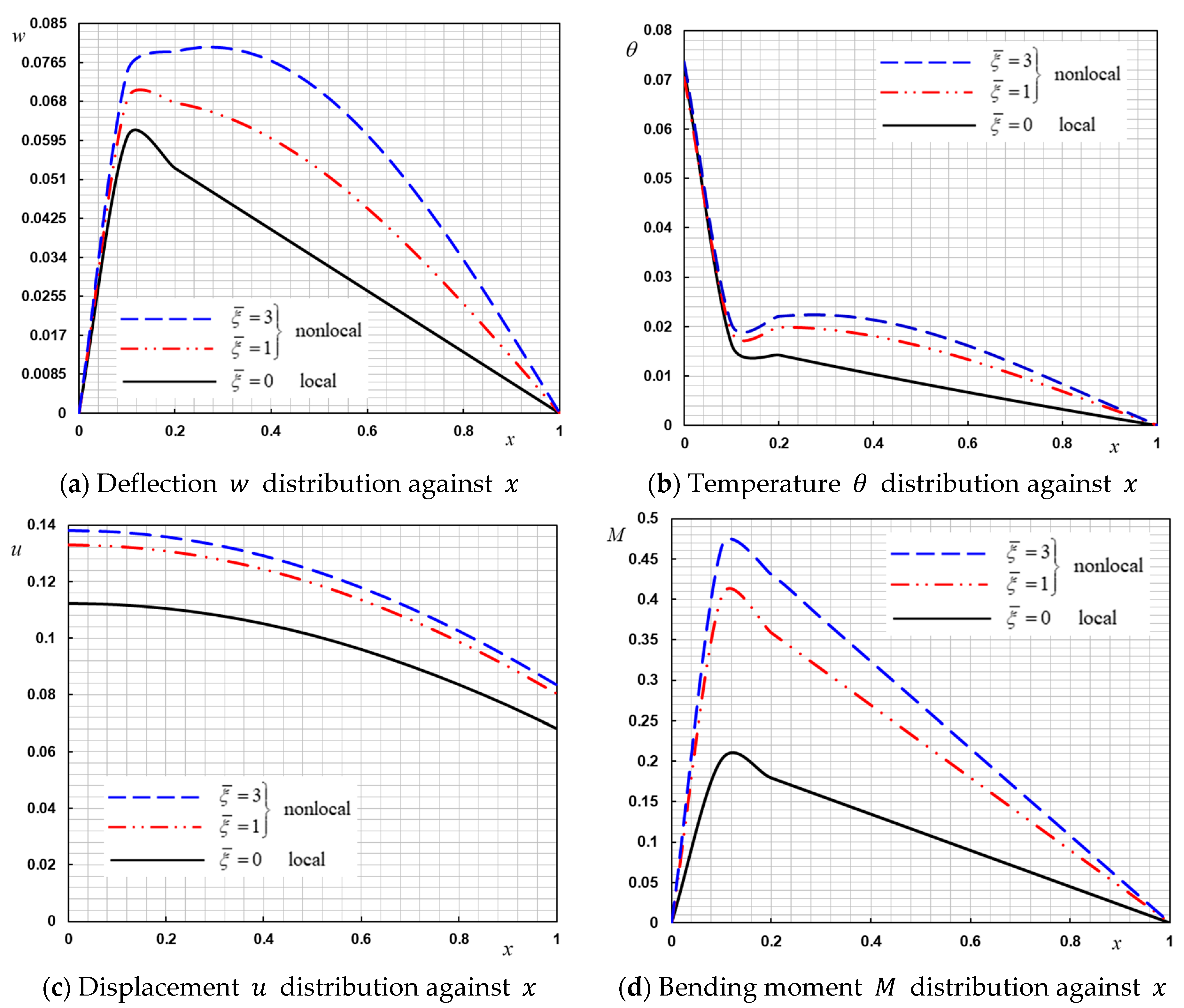
In the first case, the significance of scale coefficient on different field variables has been highlighted. The nonlocal parameter $\xi$ is obtained experimentally for different materials; for example, a conservative estimate of $\xi <4{\left(\mathrm{nm}\right)}^2$ is proposed for a single-walled carbon nanotube. In this study, the non dimensional nonlocal parameter $\xi$ was given by $\xi ={10}^{-6}$. To clarify the effect of this parameter more clearly, we will introduce a new parameter $\overline{\xi }$ ($\overline{\xi }={10}^6\xi$). The other effective parameters such as the parameter of the variability of thermal conductivity $K_1$, scale coefficient $l$, the parameters $t$, $S_1,$ and ${\tau }_0$ remain constants.

In Figure 2a–d, the numerical results are shown for various nonlocal parameter coefficients. In the case of the nonlocal model, we took $\overline{\xi }=1$ and $3$ and for the classical one, we put $\overline{\xi }=0$. The prominent effect of the non-local parameter $\overline{\xi }$ can be observed in all areas studied. The displayed figures show that, with the increases in the nonlocal scale parameter, the magnitude of the studied variables $\theta$, $w$, $u,$ and $M$ increased.

It can be observed from the figures that there is an excellent agreement between the current results and those in [19,25,50], as it can be seen that this parameter had a clear effect on all the different distributions. It is noted from figures that the peak points of the physical fields increased with the increase in the nonlocal parameter. From Figure 2a, we can see that the distribution of deflection started from zero and increased gradually until it attained the highest value at position $x=0$ and then decreased again to zero, which satisfied the conditions of the problem. As shown in Figure 2b, the temperature distribution decreased with increasing distance $x$ in the direction of the heat wave propagation, which is physically appropriate.

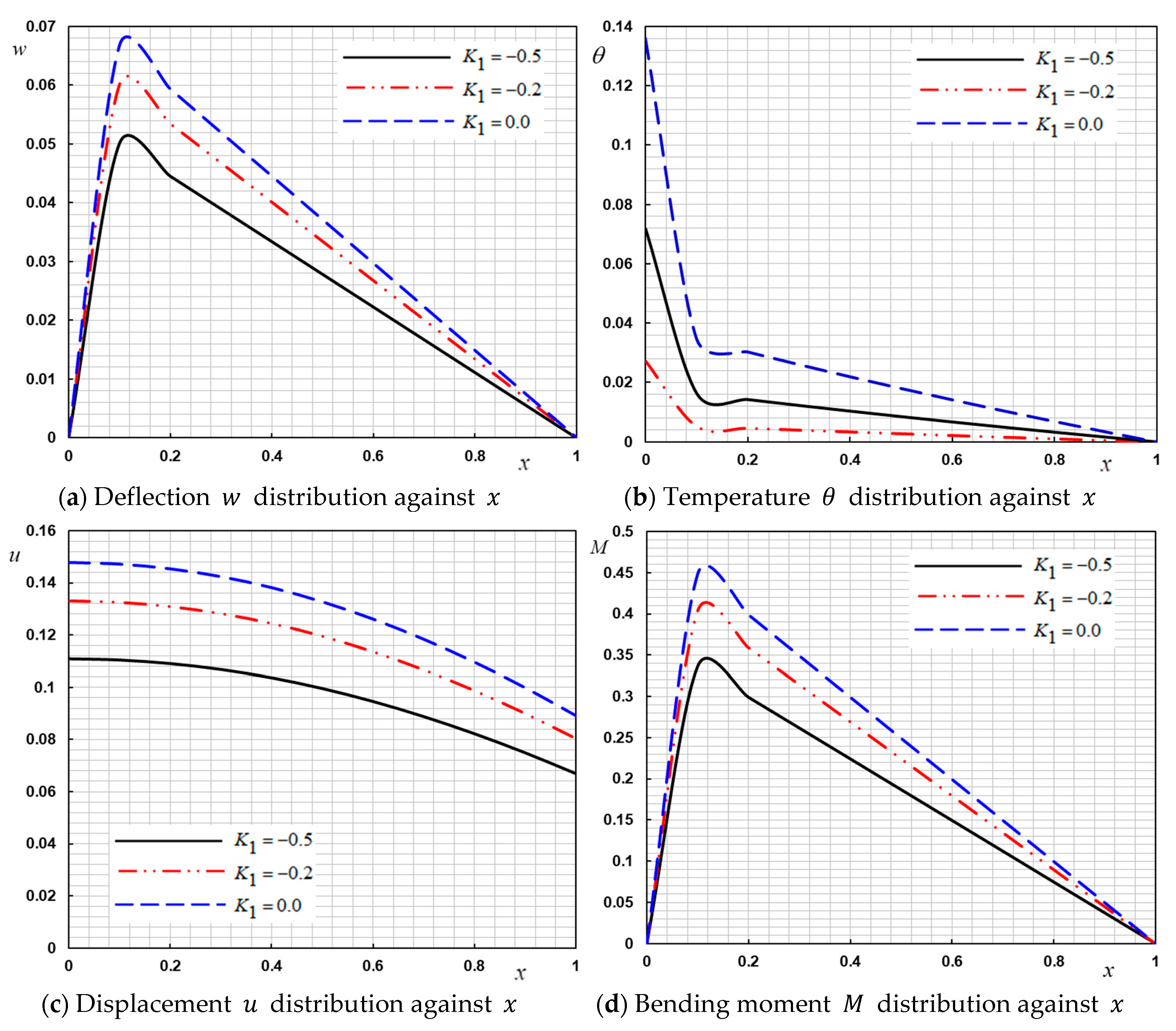
In the second case, the behavior of the field quantities under the influence of thermal conductivity variability $K=K_0\left(1+K_1\theta \right)$ was investigated. The parameter $K_0$ is the initial thermal conductivity (when thermal conductivity in independent of temperature) and the parameter $K_1$ is the small negative quantity for measuring the influence of temperature on thermal conductivity. To make comparisons and to study the effect of variability of $K$ on different distributions, we will take a third of a different value of the parameter $K_1=0,-0.2$ and $K_1=-0.5$ when parameters $\overline{\xi }$, $S_1$ and ${\tau }_0$ remain constant.

Numerical values are represented by the Figure 3a–d. We noticed that there was a noticeable difference in the values of the fields when $K_1=0.0$ compared to the values when $K_1=-0.2$ and $K_1=-0.5$. Hence, it is necessary to consider the change of the coefficient of thermal conductivity with the change of temperature when designing devices and machines. From the Figures presented, it can be seen that the curves of the different distributions of the studied functions decrease with the increase of the parameter $K_1,$ which corresponds to [51,52].

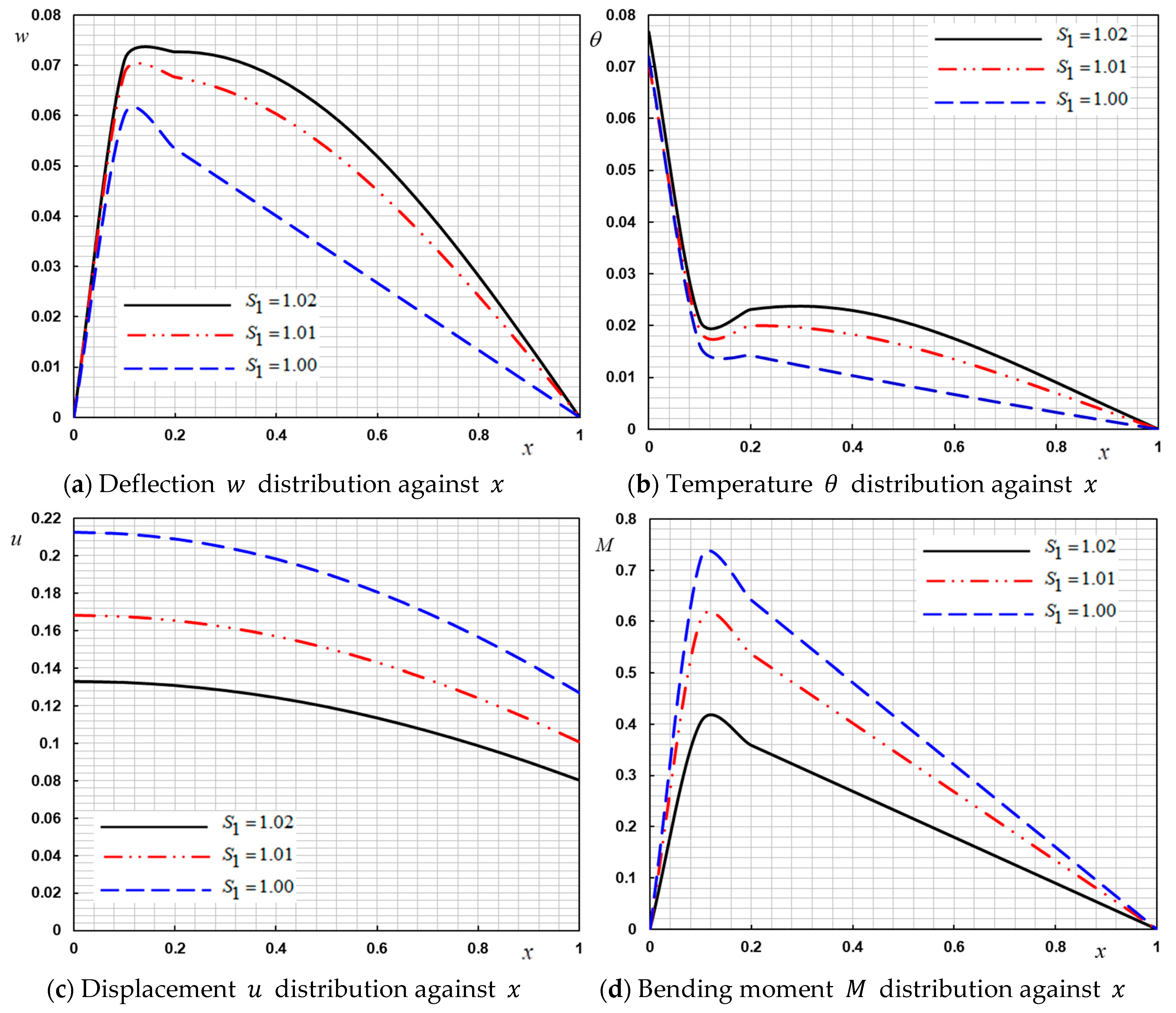
In the last case, a comparison was investigated between the MCS model and the classical continuum theory. The couple stress theory had two advantages in comparison with other classical theories. The first was that the constitutive relations included only one length scale parameter. The second one was the anti-symmetry of the curvature and the couple stress tensors. Numerical results of the field variables in the context of MCS theory are explained in 4(a–d). In the case of MCS theory, we have $S_1=1+6l^2/\left(h^2\left(1+\nu \right)\right)$ with scale coefficient $h/l=2.5$ and $\nu =0.22$. Comparisons were made for three different size-scale values $S_1=1.01$, $S_1=1.02,$ and in the absence of the effect of the small scale $S_1=1$ ($l=0$). Other effective parameters $K_1$, $\overline{\xi },$ and ${\tau }_0$ are constants. The material scale parameter of the MCS theory had a great influence on the considered fields. It is noted that the current work results were in good agreement with the results of [47,53,54]. Note, for example, that the values of deflection $w$ in the MCS model were higher compared to classical theory. The results depicted in Figure 4c are expected due to the fact that couple stress theories led to stiffening structural responses in terms of the scale parameter.

9. Conclusions

In this investigation, a thermoelastic new model for Euler–Bernoulli nanobeams was derived based on generalized thermoelasticity, modified couple stress, and nonlocal elasticity theories. Additionally, it was considered that the thermal conductivity was a linear function dependent on the temperature increment. The analysis of the state-space approach was employed to get the analytical expressions for the physical fields based on the Laplace transformations. Discussions and comparisons were made in the presence and absence of the influence of many effective parameters. The strain energy in this theory included only the antisymmetric part of the curvature and couple stress tensors resulting in a simpler form of the strain energy in comparison with other non-classical theories.

According to the results obtained from this study, we found that the effective parameters had a clear effect on thermal and mechanical behaviors. This observation is very important in the industry, especially in the design of precision devices and machines. Additionally, the current model is expected to be extremely effective in analyzing and designing of nanorods, nanotubes, and nanoscale beams under nonlinear geometry and different thermal load conditions. In addition, it can be effective in design procedures for modern nanodevices such as nanosensors and nanoscopes.

In the future, some contradictory results and some inconsistencies in the non-local flexibility approach referred to by some recent studies will be studied.

References

1. Biot, M. Thermoelasticity and irreversible thermo-dynamics. J. Appl. Phys. 1956, 27, 240–253. [Google Scholar] [CrossRef]
2. Lord, H.; Shulman, Y. A generalized dynamical theory of thermoelasticity. J. Mech. Phys. Solids 1967, 15, 299–309. [Google Scholar] [CrossRef]
3. Green, A.E.; Lindsay, K.A. Thermoelasticity. J. Elast. 1972, 2, 1–7. [Google Scholar] [CrossRef]
4. Civalek, Ö.; Demir, Ç. Bending analysis of microtubules using nonlocal Euler-Bernoulli beam theory. Appl. Math. Model. 2011, 35, 2053–2067. [Google Scholar] [CrossRef]
5. Drexler, K.E. Nanosystems: Molecular Machinery, Manufacturing, and Computation; Wiley: New York, NY, USA, 1992. [Google Scholar]
6. Kiani, K. Forced vibrations of a current-carrying nanowire in a longitudinal magnetic field accounting for both surface energy and size effects. Phys. E 2014, 63, 27–35. [Google Scholar] [CrossRef]
7. Wang, C.M.; Zhang, Y.Y.; Ramesh, S.S.; Kitipornchai, S. Buckling analysis of micro- and nano-rods/tubes based on nonlocal Timoshenko beam theory. J. Phys. D Appl. Phys. 2006, 39, 3904–3909. [Google Scholar] [CrossRef]
8. Lu, P. Dynamic analysis of axially prestressed micro/nanobeam structures based on nonlocal beam theory. J. Appl. Phys. 2007, 101, 073504. [Google Scholar] [CrossRef]
9. Farajpour, A.; Rastgoo, A. Influence of carbon nanotubes on the buckling of microtubule bundles in viscoelastic cytoplasm using nonlocal strain gradient theory. Res. Phys. 2017, 7, 1367–1375. [Google Scholar] [CrossRef]
10. Fang, D.N.; Sun, Y.X.; Soh, A.K. Analysis of frequency spectrum of laser-induced vibration of microbeam resonators. Chin. Phys. Lett. 2006, 23, 1554–1557. [Google Scholar]
11. Mashat, D.S.; Zenkour, A.M.; Abouelregal, A.E. Thermoviscoelastic vibrations of a micro-scale beam subjected to sinusoidal pulse heating. Int. J. Acous. Vibr. 2017, 22, 260–269. [Google Scholar] [CrossRef]
12. Eltaher, M.A.; Kabeel, A.M.; Almitani, K.H.; Abdraboh, A.M. Static bending and buckling of perforated nonlocal size-dependent nanobeam. Microsyst. Technol. 2018, 24, 4881–4893. [Google Scholar] [CrossRef]
13. Zenkour, A.M.; Abouelregal, A.E. Effect of ramp-type heating on the vibration of functionally graded microbeams without energy dissipation. Mech. Adv. Mat. Struct. 2016, 23, 529–537. [Google Scholar] [CrossRef]
14. Hashemi, S.H.; Behdad, S.; Fakher, M. Vibration analysis of two-phase local/nonlocal viscoelastic nanobeams with surface effects. Eur. Phys. J. Plus 2020, 135, 190. [Google Scholar] [CrossRef]
15. Marin, M.; Craciun, E.M.; Pop, N. Considerations on mixed initial-boundary value problems for micropolar porous bodies. Dyn Syst. Appl. 2016, 25, 175–196. [Google Scholar]
16. Abbas, I.; Marin, M. Analytical solution of thermoelastic interaction in a half-space by pulsed laser heating. Phys. E Low Dim Syst. Nanostruct. 2017, 87, 254–260. [Google Scholar] [CrossRef]
17. Alghamdi, N.A. The vibration of nano-beam subjected to thermal shock and moving heat source with constant speed. J. Nano Res. 2020, 61, 136–150. [Google Scholar] [CrossRef]
18. Borjalilou, V.; Asghari, M.; Taati, E. Thermoelastic damping in nonlocalnanobeams considering dual-phase-lagging effect. J. Vib. Contr. 2020, 26, 1042–1053. [Google Scholar] [CrossRef]
19. Hosseini, S.; Rahmani, O. Thermomechanical vibration of curved functionally graded nanobeam based on nonlocal elasticity. J. Therm. Stress. 2016, 39, 1252–1267. [Google Scholar] [CrossRef]
20. Romano, G.; Barretta, R. Nonlocal elasticity in nanobeams: The stress-driven integral model. Int. J. Eng. Sci. 2017, 115, 14–27. [Google Scholar] [CrossRef]
21. Abouelregal, A.E. Response of thermoelastic microbeams to a periodic external transverse excitation based on MCS theory. Microsyst. Tech. 2018, 24, 1925–1933. [Google Scholar] [CrossRef]
22. Eringen, A.C. Nonlocal polar elastic continua. Int. J. Eng. Sci. 1972, 10, 1–16. [Google Scholar] [CrossRef]
23. Eringen, A.C. On differential equations of nonlocal elasticity and solutions of screw dislocation and surface waves. J. Appl. Phys. 1983, 54, 4703–4710. [Google Scholar] [CrossRef]
24. Eringen, A.C.; Edelen, D.G.B. On nonlocal elasticity. Int. J. Eng. Sci. 1972, 10, 233–248. [Google Scholar] [CrossRef]
25. Wang, Q.; Liew, K.M. Application of nonlocal continuum mechanics to static analysis of micro- and nano-structures. Phys. Lett. A 2007, 363, 236–242. [Google Scholar] [CrossRef]
26. Romano, G.; Barretta, R.; Diaco, M.; Marotti de Sciarra, F. Constitutive boundary conditions and paradoxes in nonlocal elastic nanobeams. Int. J. Mech. Sci. 2017, 121, 151–156. [Google Scholar] [CrossRef]
27. Challamel, N.; Wang, C.M. The small length scale effect for a non-local cantilever beam: A paradox solved. Nanotechnology 2008, 19, 345703. [Google Scholar] [CrossRef]
28. Hache, F.; Challamel, N.; Elishakoff, I.; Wang, C.M. Comparison of nonlocal continualization schemes for lattice beams and plates. Arch. Appl. Mech. 2017, 87, 1105–1138. [Google Scholar] [CrossRef] [Green Version]
29. Fernández-Sáez, J.; Zaera, R.; Loya, J.A.; Reddy, J.N. Bending of Euler-Bernoulli beams using Eringen’s integral formulation: A paradox resolved. Int. J. Eng. Sci. 2016, 99, 107–116. [Google Scholar] [CrossRef] [Green Version]
30. Romano, G.; Barretta, R. Stress-driven versus strain-driven nonlocal integral model for elastic nano-beams. Compos. Part B 2017, 114, 184–188. [Google Scholar] [CrossRef]
31. Barretta, R.; Diaco, M.; Feo, L.; Luciano, R.; de Sciarra, F.M.; Penna, R. Stress-driven integral elastic theory for torsion of nano-beams. Mechanics 2018, 87, 35–41. [Google Scholar] [CrossRef]
32. Bahar, L.Y.; Hetnarski, R.B. State space approach to thermoelasticity. J. Stress 1978, 1, 135–145. [Google Scholar] [CrossRef]
33. Sherief, H. State space formulation for generalized thermoelasticity with one relaxation time including heat sources. J. Stress 1993, 16, 163–180. [Google Scholar] [CrossRef]
34. Anwar, M.; Sherief, H. State space approach to generalized thermoelasticity. J. Therm. Stress. 1988, 11, 353–365. [Google Scholar] [CrossRef]
35. Zenkour, A.M.; Abouelregal, A.E. Thermoelastic vibration of temperature-dependent nanobeams due to rectified sine wave heating—A state space approach. J. Appl. Comp. Mech. 2019, 5, 299–310. [Google Scholar]
36. Akgöz, B.; Civalek, O. A size-dependent shear deformation beam model based on the strain gradient elasticity theory. Int. J. Eng. Sci. 2013, 70, 1–14. [Google Scholar] [CrossRef]
37. Wang, B.; Zhao, J.; Zhou, S. A micro scale timoshenko beam model based on strain gradient elasticity theory. Eur. J. Mech. A Solids 2010, 29, 591–599. [Google Scholar] [CrossRef]
38. Yang, F.; Chong, A.C.M.; Lam, D.C.C.; Tong, P. Couple stress based strain gradient theory for elasticity. Int. J. Solid Struct. 2002, 39, 2731–2743. [Google Scholar] [CrossRef]
39. Akgoz, B.; Civalek, O. Strain gradient elasticity and modified couple stress models for buckling analysis of axially loaded micro-scaled beams. Int. J. Eng. Sci. 2011, 49, 1268–1280. [Google Scholar] [CrossRef]
40. Reddy, J.N.; Kim, J. A Nonlinear Modified couple stress-based third-order theory of functionally graded plates. Compos. Struct. 2012, 94, 1128–1143. [Google Scholar] [CrossRef]
41. Farokhi, H.; Ghayesh, M.H.; Amabili, M. Nonlinear dynamics of a geometrically imperfect microbeam based on the modified couple stress theory. Int. J. Eng. Sci. 2013, 68, 11–23. [Google Scholar] [CrossRef]
42. Şimşek, M. Dynamic analysis of an embedded microbeam carrying a moving micro-particle based on the modified couple stress theory. Int. J. Eng. Sci. 2010, 48, 1721–1732. [Google Scholar] [CrossRef]
43. Romano, G.; Barretta, R.; Diaco, M. Micromorphic continua: Non-redundant formulations. Contin. Mech. Thermodyn. 2016, 28, 1659–1670. [Google Scholar] [CrossRef]
44. Barbagallo, G.; Madeo, A.; d’Agostino, M.V.; Abreu, R.; Ghiba, I.-D.; Neff, P. Transparent anisotropy for the relaxed micromorphic model: Macroscopic consistency conditions and long wave length asymptotics. Int. J. Solids Struct. 2017, 120, 7–30. [Google Scholar] [CrossRef]
45. Neff, P.; Madeo, A.; Barbagallo, G.; d’Agostino, M.V.; Abreu, R.; Ghiba, I.-D. Real wave propagation in the isotropic-relaxed micromorphic model. Proc. R. Soc. A 2017, 473, 2197. [Google Scholar] [CrossRef] [PubMed]
46. Hadjesfandiari, A.R.; Dargush, G.F. Couple stress theory for solids. Int. J. Solid. Str. 2011, 48, 2496–2510. [Google Scholar] [CrossRef] [Green Version]
47. Kumar, R. Response of thermoelastic beam due to thermal source in modified couple stress theory. CMST 2016, 22, 95–101. [Google Scholar] [CrossRef] [Green Version]
48. Alifanov, O.M. Inverse Heat Transfer Problems; Springer: Berlin, Germany, 1994. [Google Scholar]
49. Zhang, Z.M. Nano/Microscale Heat Transfer; McGraw-Hill: New York, NY, USA, 2007. [Google Scholar]
50. Tzou, D. Macro-to-Micro Heat Transfer; Taylor & Francis: Washington, DC, USA, 1996. [Google Scholar]
51. Ebrahimi, F.; Barati, M.R. Magnetic field effects on nonlocal wave dispersion characteristics of size-dependent nanobeams. Appl. Phys. A 2017, 123, 81. [Google Scholar] [CrossRef]
52. Li, C.; Guo, H.; Tian, X. Time-domain finite element analysis to nonlinear transient responses of generalized diffusion-thermoelasticity with variable thermal conductivity and diffusivity. Int. J. Mech. Sci. 2017, 131, 234–244. [Google Scholar] [CrossRef]
53. Dogonchi, S.; Ganji, D.D. Convection–radiation heat transfer study of moving fin with temperature-dependent thermal conductivity, heat transfer coefficient and heatgeneration. Appl. Therm. Eng. 2016, 103, 705–712. [Google Scholar] [CrossRef]
54. Mohandes, M.; Ghasemi, A.R. Modified couple stress theory and finite strain assumption for nonlinear free vibration and bending of micro/nanolaminated composite Euler–Bernoulli beam under thermal loading. Proc. Inst. Mech. Eng. Part. C J. Mech. Eng. Sci. 2016, 231, 4044–4056. [Google Scholar] [CrossRef]
Figure 1. Schematic illustration of the nanobeam.
Symmetry 12 01276 g001
Figure 2. The physical field variables versus x for different values of nonlocal parameter ξ .
Symmetry 12 01276 g002
Figure 3. The physical field variables versus x when thermal conductivity K is temperature-dependent.
Symmetry 12 01276 g003
Figure 4. The physical field variables versus x for different values of small scale parameter l .
Symmetry 12 01276 g004