Using Fuzzy Sets and Markov Chain Method to Carry out Inventory Strategies with Different Recovery Levels

Abstract

In this study, we first analyze the usability of recycling products, and use the fuzzy set method to determine the main impact on recycling items and their corresponding weights by using the Analytic Hierarchy Process (AHP) to identify various impact recycling levels. The Group Decision Supporting System (GDSS) determines the test standards for the recycling rating. It provides a convenient way for recyclers or manufacturers to classify their own products and use fuzzy numbers to select a set of test standards. It can deduce the recovery rate and remanufacturing rate of different recycling processing levels through the Markov chain model to find out the inventory model and total cost. In the numerical analysis, we found that a recycling rate of more than 90% is probably a necessary decision. Since the processing cost of the 100% recovery rate is doubled, the inventory level and total cost will increase with it. Therefore, this study was combined with the reverse logistics method to find the appropriate decision-making strategy and plan, such as the optimal inventory level and recovery rate.

1. Introduction

In the past decade, due to the increasing demand for green products worldwide, the issue of green productivity has gradually attracted attention. Some of the latest laws passed in Europe are examples of such strong requirements, including the Waste Electrical and Electronic Equipment Directive 2002/96/EC (WEEE) and Restriction of Hazardous Substances (RoHS) standards, which have placed great pressure on product designers and manufacturers to produce greener and cleaner products. However, if individual companies respond to these requests, the problem may not be solved effectively. Instead, the trend is to provide an overall product supply chain operation strategy. Under the competition of the global economy and environment, the product life cycle seems to be shorter than before. The competition and survival of the company must incorporate the reverse supply chain into the management. On the other hand, environmental protection will also affect the corporate image. Therefore, for the sake of ecological protection and sustainable business operation, the integration of suppliers and buyers in successful supply chain management is one of the main successful methods.

Reverse logistics represents a series of logistics activities that recover used products from consumers and reuse this resource in the market. In the past, the reverse logistics was mostly based on the product production and recycling of Thierry M.C (1995) [1]. Fleischmann (1997) [2]; Carter and Ellram (1998) [3]; Guide (2002) [4] and other studies also revealed that the distribution cost of recycling reverse logistics is often higher than that of forward logistics. For the returned products, there are also irregular channels in terms of transportation, storage, processing, and management, which adds a lot of complexity and uncertainty to the supply chain. Therefore, LA Zadeh (1973) [5] obtains the correct result through the approximation reasoning process, which is very similar to the human brain “process is fuzzy, the conclusion is clear” thinking mode, so Jang et al. (1996) [6] is widely used in various intelligent systems in different fields.

Then, Zipkin (1993) [7] used the Markov chain to develop a model of dynamic interest rate evaluation of real estate mortgage-backed securities. Aase (2001) [8] uses the Markov model to provide an assessment theory for the catastrophe’s long-term contract or derivative commodity insurance. Ching et al. (2002) [9], Naranjo, L, et al. (2019) [10], Lizbeth Naranjo, et al. (2020) [11] apply the Markov chain to develop a multivariable Markov chain to predict customer demand. The reverse logistics environment still needs to integrate the upstream and downstream supply chains, so Lin and Lin (2011) [12], Lin and Su (2013) [13], Verhoeven and Sinn (2018) [14] and Ho and Lin (2020) [15], for the overall logistics supply chain with the lowest overall cost as the target, consider the defective products level, inventory cost, transportation and other expenses. To aim at the overall logistics supply chain with the lowest overall total cost, we have to consider the cost of bad goods, inventory cost, transportation and so on. Minner and Kiesmüller (2012) [16] explored the closed supply chain in a dynamic model. Xin et al. (2019) [17] and Kannan et al. (2020) [18] used fuzzy theory to solve the closed supply chain model.

In this paper, we extend the single-item single-location inventory system of Erwin et al. (1996) [19] with multiple-items and multiple-periods. We consider the recovery rate and remanufacturing rate of different recycle processing levels and combine reverse logistics methods to develop a set of mathematical inventory models. In the results of numerical analysis, we show the effects of different recycling levels.

2. Model Description

The impact of environmental responsibility on the manufacturing business model is becoming higher and higher, and the products produced by different industries have different environmental loads. Moreover, the life of the product will vary with the frequency of use or the environment, resulting in differences in surface luminosity, short circuit, damage, or scrapping process. Products produced in different industries have different environmental hazards and different levels of recycling. This study considers different recycling levels for a single project as shown in Figure 1 (Thierry, M., et al. (1995) [1]). In other words, the recycling status can be roughly divided into transfer, polishing, maintenance, remanufacturing, crushing, burying, incineration.

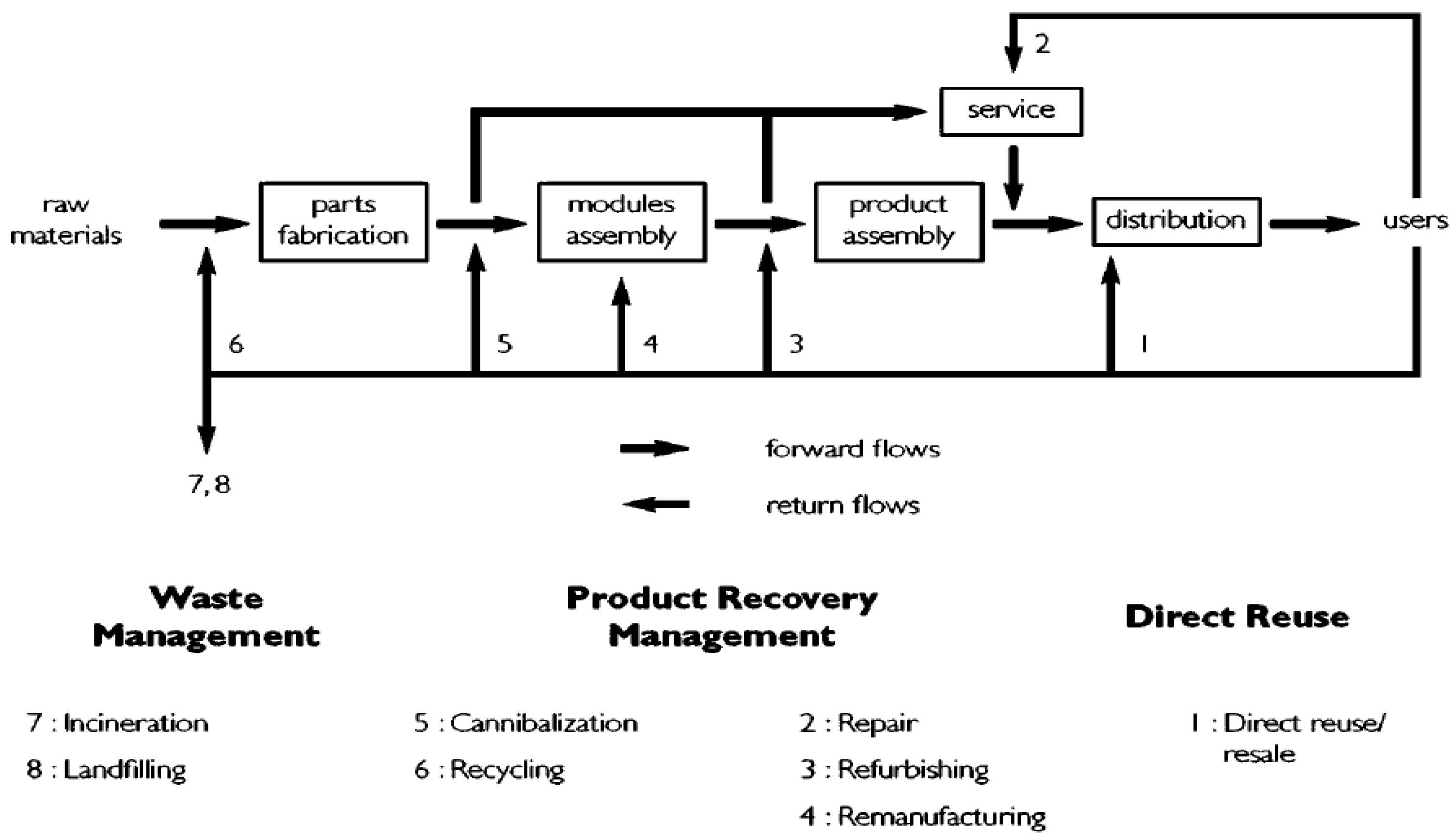
The impact of environmental responsibility on the manufacturing business model is becoming higher and higher, and the products produced by different industries have different environmental loads. Moreover, the life of the product will vary with the frequency of use or the environment, resulting in differences in surface luminosity, short circuit, damage, or scrapping process. Products produced in different industries have different environmental hazards and different levels of recycling. This study considers different recycling levels for a single project as shown in Figure 1 (Thierry, M., et al. (1995) [1]). In other words, the recycling status can be roughly divided into transfer, polishing, maintenance, remanufacturing, crushing, burying, incineration.

Due to the different attributes of various products, the degree of recycling treatment is also different. Some products do not even have maintenance or remanufacturing operations. Therefore, the various process levels and recovery types are summarized in

Table 1. Reverse logistics processing and recovery type.

Processing Level	Recovery Type	Example
Repairing (Refresh)	Used/second hand	Steam locomotive, etc.
Remanufacturing (Reproduction)	Element/components	Electronic parts
Recycling (Reuse)	Raw material	Iron, plastic pellets
Disposal	Waste residue	Waste slag

.

The symbol definitions are shown below:

Symbol definition:

λi	Stage i repair or remanufacturing rate;
γi	Stage i recovery rate;
Vi	The degree of different influencing factors;
W	influence factor weight;
E	Recursive probability matrix;
s	Safety stock;
Q	Inventory (Economic order quantity);
Pi	Stage I probability;
R	Order maintenance items;
Li	Expected number of each recycling level i system;
θ	Lagrangian Correction factor;
h	holding cost;
π	setup cost;
τ	lead time;
A	unit cost.

3. Mathematical Model

3.1. Using Group Decision Support System (GDSS) and Fuzzy Matrix to Determine the Fuzzy Classification Principle for the Corresponding Recycling Rating

In this study, we assumed that there were t recycle processing levels. We first used a group decision support system (GDSS) as the measurement procedure to determine the test standard, $\mathrm{C}=\{c_1,\dots ci\}$, the test standard items. The recycling score was expressed as a full score of 100 points, and the rating given for each recycling level was $M^{\prime }=\{m_{i1},\dots ,m_{in}\};m_{ij}\in \{0,100\},(i=1,..,t;j=1,\dots ,n)$. m_ij denotes the subjective weight of a group of experts. It represents an integer value between 0 to 100 for the weight of experts. The experts from different recycling sites will use the fuzzy matrix from [0, 100] generating a rating score of the recycling manufacturer, and then use the GDSS to select the test standard.

We assumed t as the recycle processing levels (input), each of which had a different degree of influence factor (u_i), u_i = {1~100} where u_i represents the actual use status of different impact factors (degree of damage, processing costs and the number of miles traveled). The results were standardized from 1 to 100. ${\mu }_{gi}(m_i^{\prime })$ denotes the average rating score from the experts of different recycling sites. We used $({\mu }_{g1}(m_i^{\prime }),{\mu }_{g2}(m_i^{\prime }),\dots ,{\mu }_{gd}(m_i^{\prime }))$ = AHP/u_i or the GDSS model to build a fuzzy matrix. We used AHP level analysis to divide by different impact factors (ui), in order to carry out the standardization procedure, and the result obtained was the standardized comparative matrix. To calculate of the fuzzy matrix, we determined the fuzzy classification principle, which was then able to correspond to the final rating of the recovery. By simplified conversion procedures, we used $(e_{i1}\dots ..e_{id})$ instead of $({\mu }_{g1}(m_i^{\prime }),{\mu }_{g2}(m_i^{\prime }),\dots ,{\mu }_{gd}(m_i^{\prime }))$ to simplify the formula, as shown in Equation (1):

$$E=\left[\begin{array}{c}{e}_{11} e_{12}\dots e_{1d}\\ e_{21} e_{22} \dots e_{2d}\\ \dots \dots \\ {\mathrm{e}}_{\mathrm{n}1} e_{n2} \dots e_{nd}\end{array}\right]={(e_{ij})}_{(i=1,2,\dots \mathrm{n}; j=1,2,\dots \mathrm{d})}$$

(1)

For the analysis, we defined the weight of each influencing factor as $\tilde{W}=\{\frac{w_1}{u_1},\dots ..,\frac{w_t}{u_t}\};{\displaystyle {\sum }_{i=1}^t{w}_i=}1$, and $\tilde{P}=\{u_1,\dots ..,u_t\}$ represented a set of fuzzy influencing factors. The rating of each recycling level was expressed as 1–100, and these scores were assigned back to the corresponding test standard items. For example, $\tilde{W}=\{\frac{0.5}{\mathrm{Degree} \mathrm{of} \mathrm{damage}},\frac{0.3}{\mathrm{Processing} \cos \mathrm{ts}},\frac{0.2}{\mathrm{mileages}}\}$ = $\{\frac{0.5}{1\dots 100},\frac{0.3}{1\dots 100},\frac{0.2}{1\dots 100}\}$; finally, we got the Equation (2), as shown below:

$$Y=W\times E=\left(w_1 w_2 \dots w_n\right)\times \left[\begin{array}{c}{e}_{11} e_{12} \dots e_{1d}\\ e_{21} e_{22} \dots e_{2d}\\ \dots \dots \\ {\mathrm{e}}_{\mathrm{n}1} e_{n2} \dots e_{nd}\end{array}\right]$$

(2)

We standardized from the evaluation of the Y vector, determining the fuzzy classification principle $y_i=\max (y_1\dots y_d)$, which was able to correspond to the final rating of the recovery.

3.2. An Inventory System with Multiple-Processing Levels and Multiple-Period Returns

Comparing our system to the single-item system (Figure 2) by Erwin et al. [19], we developed approximation procedures of multiple-processing levels and multiple-period returns (Figure 3) to show the effects of different recycling levels on inventory cost.

In practice, product recycling will change its characteristics over time, so we assumed the time point {t ∈ T} (where T was the set of time points), and let X_t be the recovery state of the system at t. In most cases, although we did not know the certain value of the recovery state of the system at time t, it was a random variable, and a random recovery process {X_t} had the Markov property, Pr (X_t+1 = j|X_t = i, X_t−1 = I − 1, X_t−2 = i − 2, X_t−3 =i − 3, ….., X₀ = 0) = P_r (X_{t+1 =} j|X_{t =} i), to calculate the inventory level with a continuous time Markov chain (Pawel et al. (2019) [20]).

Demand reduced the inventory level. When the inventory reached safety stock s, it would directly increase the inventory level to s + Q. Recycling increased the inventory level and the Markov chain was ergodic if the λ reproduction rate < γ recovery rate, and the central limit distribution of the inventory level tended to be a stable distribution (Erwin et al. [19]).

From the cyclic transfer process shown as Figure 4, we could develop the Markov chain long-term stability matrix, as shown in Equation (3) (Yousif et al. (2020) [21]), which considered the continuous transfer, and the expansion and transfer, of the previous period and the next period.

Products were scrapped under long-term stability, P equals

$$P=\left[\begin{array}{ccccc}1-{\displaystyle \sum {\gamma }_i}& {\gamma }_1& {\gamma }_2& {\gamma }_3& {\gamma }_4\\ {\lambda }_1& 1-{\lambda }_1& 0& 0& 0\\ 0& {\lambda }_2& 1-{\lambda }_2& 0& 0\\ 0& 0& {\lambda }_3& 1-{\lambda }_3& 0\\ 0& 0& 0& {\lambda }_4& 1-{\lambda }_4\end{array}\right]$$

(3)

From Figure 4, we expanded the single-item single-location inventory system to the multiple-period, multiple-processing level inventory system under different safety stocks (s) and different inventory levels (Q), as shown in Figure 5.

After the inventory levels of different items in different periods went through the Markov cycle conversion process during n items r recycle, they gradually converged to form a steady-state inventory level function I(T), (that is, ${\widetilde{\mathsf{{\rm I}}}}^n(t)+{\widetilde{\mathsf{{\rm I}}}}^r(t)=I(t)+k$) so that after an indefinite Markov conversion, the expected inventory level was as follows; k was constant, E(I_i(∞)) = (s + 1 + $\frac{Q-1}{2}$ + L_i), L_i was the expected number of systems for each recycling level i.

According to Erwin et al. [19], before the expected replenishment quantity is filled, F(s,τ) represents the average value µτ = (λ − γ)τ and variance στ= (λ − γ)τ of the expected excess demand exceeding the normal distribution s-R. The (λ − γ)/Q denotes the average order quantity per unit time, so the average order cost is equal to A(λ − γ)/Q. We can also get the total cost function, K(s, Q); if converted into the average order quantity per unit time of each recycling processing station, $\frac{\mathrm{L}}{\gamma Q}$, the average order cost is equal to A($\frac{{\mathrm{L}}_{\mathrm{i}}}{{\gamma }_{i}Q}$). The revised total cost function is shown below in Equation (4).

$$\mathrm{K}(\mathrm{s},\mathrm{Q})=\mathrm{A}(\frac{\mathrm{L}}{\gamma Q})+(\mathsf{\pi }+\mathrm{h})\frac{F{(s,\tau )}^2}{2Q}+\mathrm{h}[(\mathrm{s}+1+\frac{Q-1}{2}+\mathrm{L})-\mathrm{R}-(\frac{\mathrm{L}}{\lambda })\mathsf{\tau }]$$

(4)

Assuming that the resource limits for all kinds of recycling processes are the same, the equation is as follows:

$$\mathrm{Qi}\ast =\sqrt{\frac{\pi +h}{h}F{(s\ast ,\tau )}^2+\frac{2\gamma A}{h{\mathrm{L}}_{\mathrm{i}}}}$$

(5)

Assuming that all resource limits for various recycling processes are different, the following equation is obtained using the Lagrangian function:

$$\mathrm{Qi}\ast =\sqrt{\frac{F{(s\ast ,\tau )}^2(\pi i+hi)+2(\frac{{\gamma }_i}{\mathrm{L}\mathrm{i}})Ai}{hi+2\theta wi}}$$

(6)

${\displaystyle \sum _{i=1}^{n}wiQi\ast }$ = W(resource limits), θ is the correction factor of the Lagrangian.

This leads to another total cost function of K2(s,Q). Using the approximate value, the optimal Qi* (Equation (7)) value of the various inventory of different recycling processes are calculated as follows:

$$\mathrm{Qi}\ast =\sqrt{((\pi +h){\displaystyle \underset{0}{\overset{\tau }{\int }}F(s\ast ,\tau )dt+A)}\frac{2\gamma }{h\times Li}}$$

(7)

The Qi * value of different resource limits for various kinds of inventory for different recycling processes is calculated as follows. The model is shown (Equation (8)) and the optimal value for S is shown (Equation (8)):

$$\mathrm{Qi}\ast =\sqrt{((\pi +h){\displaystyle \int }F(s\ast ,\tau )dt+A)\frac{2\gamma }{h\times Li+2\theta wi}}$$

(8)

${\displaystyle \sum _{i=1}^{n}wiQi\ast }$ = W(Resource limit), θ is the Lagrangian correction factor,

In addition, s* is the optimal value for S, which must meet:

$$-\sqrt{\frac{dF(s,t)}{ds}}=\frac{h}{\pi +h}.\frac{LiQ}{\gamma }$$

(9)

Muckstadt and Sapra (2010) [22] roughly estimated that the net inventory is normally allocated. Here, they determined the steady-state inventory level and demand and the time before the repair station output is short. Consequently, they acquired different equations for the expected replenishment quantity. The drawback of their analysis is that the net inventory has asymptotic characteristics, which sometimes do not conform to actual behavior.

If Erwin [19] compares the desired demand value to λ and the recovery flow expectation value γ, the expected value of the expected recovery flow rate corresponding to only the correct demand flow rate is λ-γ. Obviously, the uncertain recovery flow rate will increase the cost and height handle of the variability process. Moreover, when γ tends to λ, the average cost will tend to be infinite. Reducing this surge in total cost is a waste strategy to reduce the recovery rate.

4. Numerical Analysis

In view of the fact that various products do not have a recycling grade, and the product recycling grade process mechanism and its recycling grade are not easy to judge from their appearance, this article takes the car as an example, divides the car recycling grade into four grades, and uses a group decision support system (GDSS) as a measurement procedure and fuzzy matrix calculation. The preliminary results of the comparison of 20 vehicles from the sale of second-hand cars, car repair shops to decomposition sites are suggested to use different clusters of vehicles and categorize each vehicle’s recycling data in different processing sites.

The test standard items generated by GDSS, the results are seven major items, C = {mileage, processing cost, damage degree, vehicle age, processing time, speed performance, functionality}

According to their preferences, experts in various fields (sales, car repairs, dismantling of parts, scrapping) will use the [0,100] fuzzy method to score the car for recycling. After the GDSS calculation, for the resulting preference vector u, u = (0.97, 0.972, 0.98, 0.81, 0.832, 0.32, 0.182). Next, the three main popular test standards were selected, and the set was changed to C = {damage, processing cost, mileage}. In order to establish the above semantic and discriminatory issues, according to the opinions of experts in various automobile recycling yards, the following guidelines were formulated for the process of automobiles (

Table 2. Guidelines for the process of automobiles.

Item	Repair	Remanufacture	Recycling	Disposal
Level of damage	L(1~33)	L(1~33)	M(34~67)	H(68~100)
Processing costs	L	M, H	L, M	L, M, H
Mileage	L	M	M, H	H

).

Then, the important scores of 1~9 were compared to each other to get the comparison relationship matrix (shown below):

$$\mathrm{AHP}=\left[\begin{array}{ccccc}1& 1& 1/3& 4& 5\\ 1& 1& 1/3& 5& 5\\ 3& 3& 1& 7& 7\\ 1/4& 1/5& 1/7& 1& 1/3\\ 1/5& 1/5& 1/7& 3& 1\end{array}\right]$$

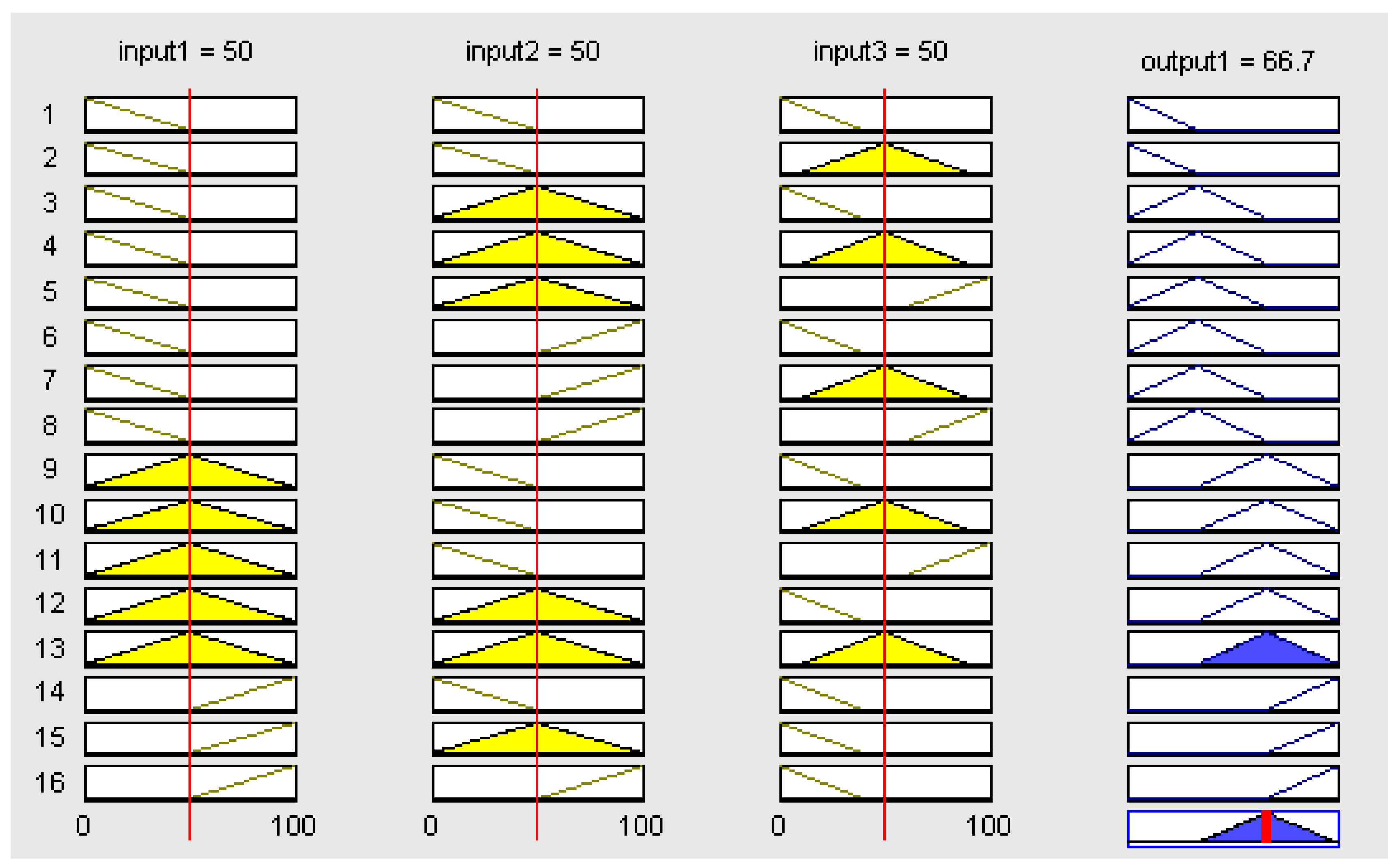
Then, we calculated the relevant weight through GDSS (normalized), got W = (0.205502, 0.214881, 0.475251, 0.042013, 0.062352), and $W_1+W_2+W_3+W_4+W_5=1$. In the rating part, it was divided into four levels: D: disposal, S: reuse, R: remanufacture, E: repair. The membership function was defined as follows:

$$\begin{array}{l}\mu D(u)=\{\begin{array}{c}1\\ (60-u)/5\\ 0\end{array}\begin{array}{c}\\ \\ \end{array}\begin{array}{c}0\le u\le 55\\ 55<u\le 60\\ 60<u\le 100\end{array}\begin{array}{cccc}& & & \end{array}\mu \mathrm{R}(u)=\{\begin{array}{c}0\\ (u-70)/5\\ 1\\ (85-u)/5\\ 0\end{array}\begin{array}{c}\\ \\ \\ \\ \end{array}\begin{array}{c}0\le u\le 70\\ 70<u\le 75\\ 75<u\le 80\\ 80<u\le 85\\ 90<u\le 100\end{array}\\ \mu \mathrm{S}(u)=\{\begin{array}{c}0\\ (u-60)/5\\ 1\\ (80-u)/10\\ 0\end{array}\begin{array}{c}\\ \\ \\ \\ \end{array}\begin{array}{c}0\le u\le 60\\ 60<u\le 65\\ 65<u\le 70\\ 70<u\le 80\\ 80<u\le 100\end{array}\begin{array}{cccc}& & & \end{array}\mu \mathrm{E}(u)=\{\begin{array}{c}0\\ (u-80)/10\\ 1\end{array}\begin{array}{c}\\ \\ \end{array}\begin{array}{c}0\le u\le 80\\ 80<u\le 90\\ 90<u\le 100\end{array}\end{array}$$

The established weights for triangular fuzzy numbers input variables input1, input2, input3, respectively, indicate the degree of damage, processing cost, mileage, and output indicates the classification of the recycling process shown in Figure 6.

Assuming that each car is scored by experts and scholars, the following matrix (E) shows the test results obtained by the car.

$$E=\left[\begin{array}{cccc}0.06& 0.8& 0.14& 0\\ 0& 0.74& 0.26& 0\\ 0& 0.94& 0.06& 0\\ 0& 0& 1& 0\\ 0& 0& 0.3& 0.7\end{array}\right]$$

Using the weights obtained before, the result of calculating the vector yi takes the maximum value, and maps to each level to correspond to which grade the product should be; the mark value is shown below.

$$\begin{array}{ll}Y& =W\times E=(0.205502,0.214881,0.475251,0.042013,0.062352)\times \left[\begin{array}{cccc}0.06& 0.80& 0.14& 0\\ 0& 0.74& 0.26& 0\\ 0& 0.94& 0.06& 0\\ 0& 0& 1& 0\\ 0& 0& 0.3& 0.7\end{array}\right]\\ & =(0.01233,0.770150, 0.173873, 0.043647)\end{array}$$

Y is a vector matrix, representing y1, y2, y3, y4 (Repairing, Remanufacturing, Reuse, Disposal, respectively). Y is the final corresponding evaluation score obtained through the fuzzy classification results; where y2 is the highest evaluation score, which means that the product Remanufacturing has the highest relative importance. Finally, the obtained product is y2, and the corresponding grade is R, which means that the car should be listed as reuse.

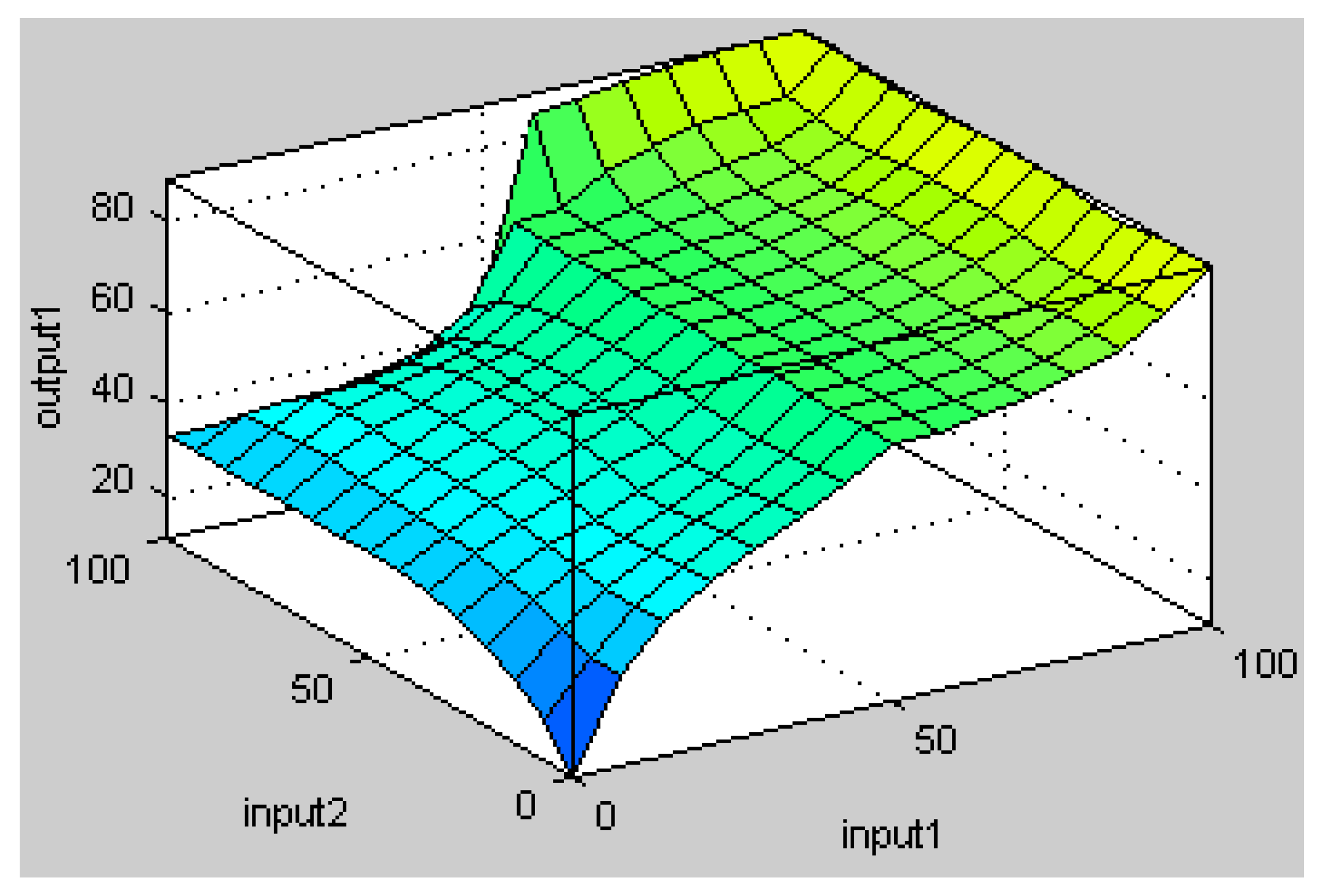
In addition, in Figure 7 shown below, Input1 and Input2, respectively, indicate the degree of damage and processing cost that affect the output recovery processing level.

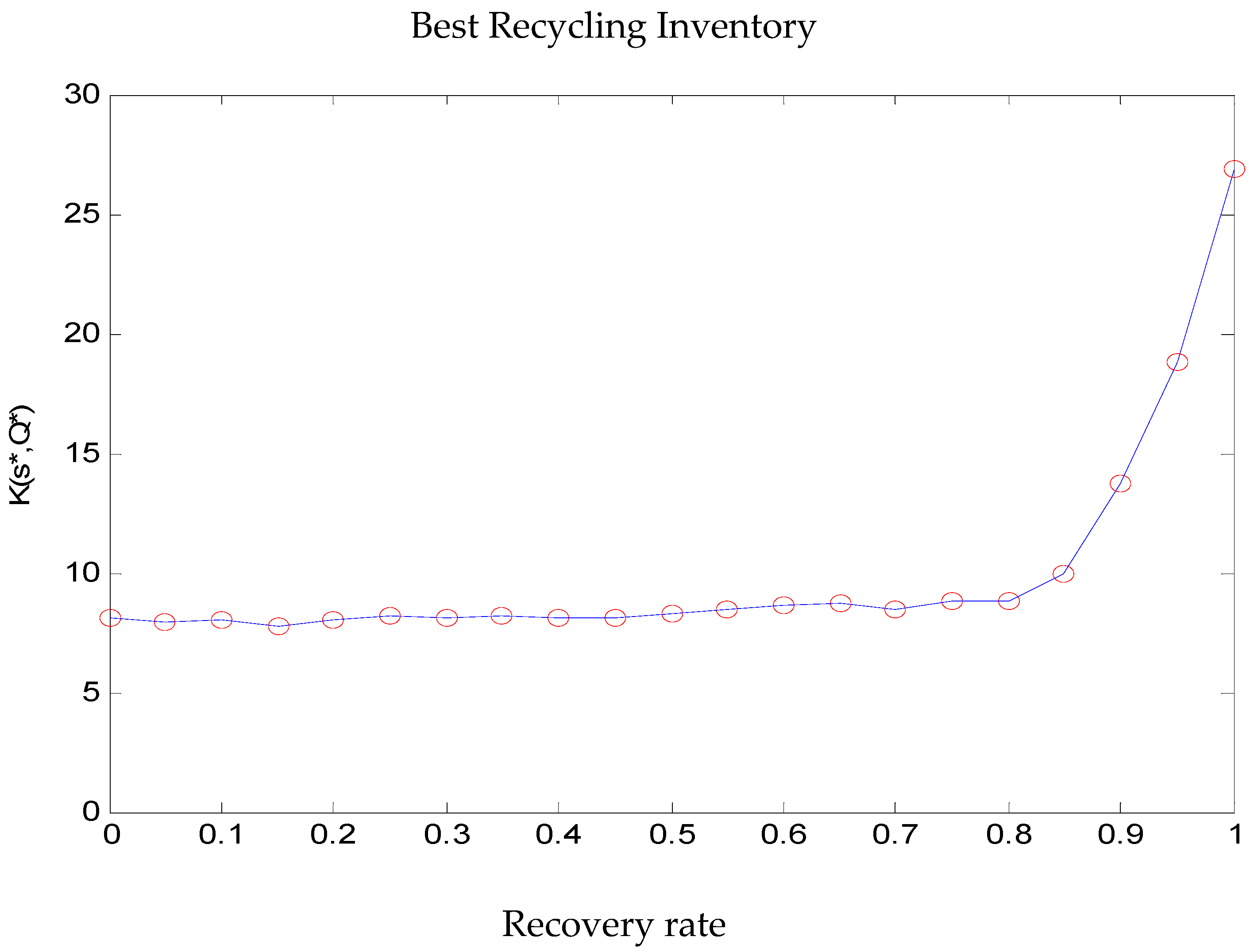
Next, we used Matlab software to show the single-item, single-location inventory system by Erwin et al. (1996) and assumed that if the holding cost h is 1, then the cost λ = 1, the unit cost A = 10, the setting cost π = 10 and the pre-processing time τ = 10. A trend chart of total inventory cost is shown in Figure 8.

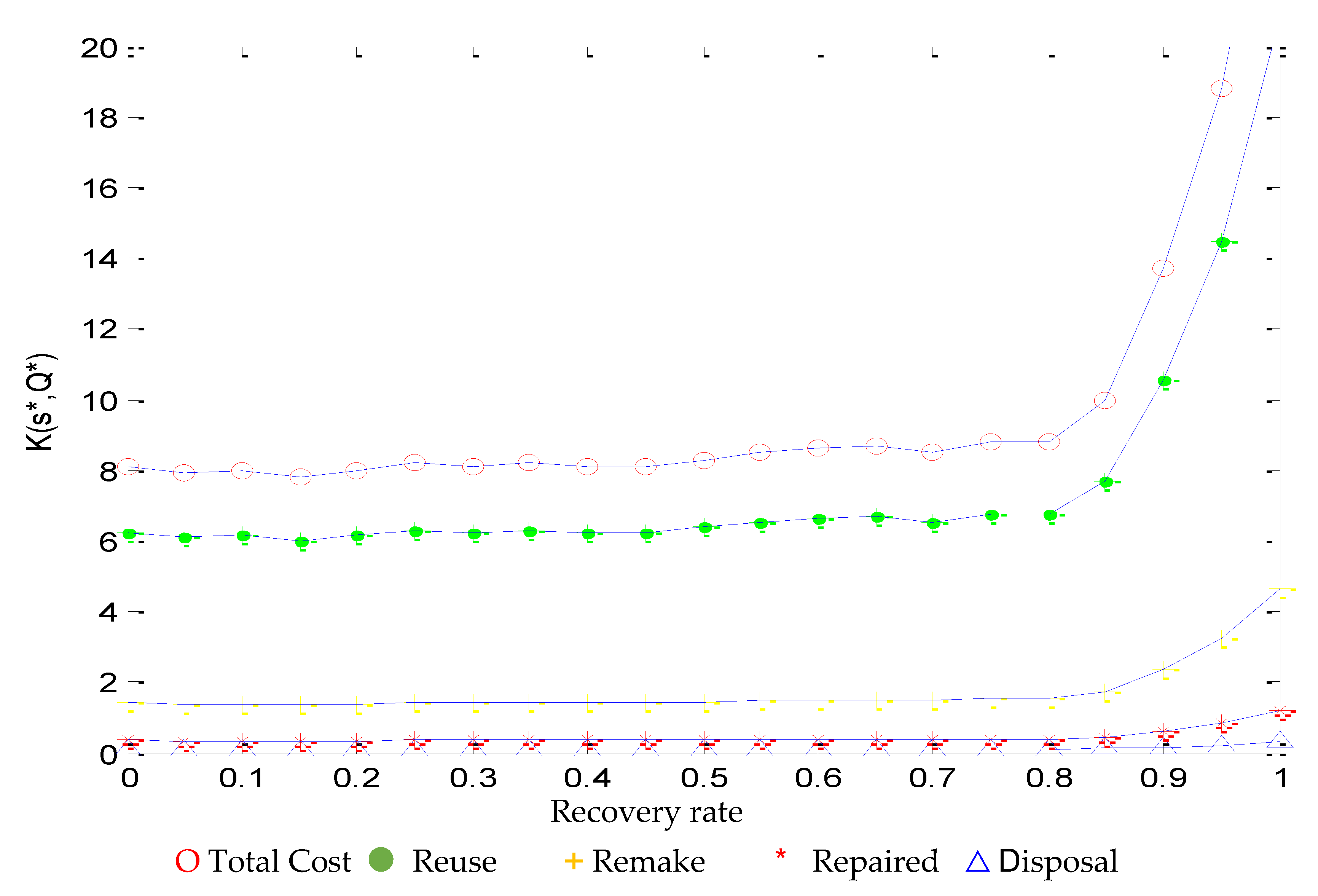
We used the parameters derived from fuzzy theory (disposal, reuse, remanufacture, repair) = (0.012330, 0.770150, 0.173873, 0.043647) in the inventory formula Equation (9). Figure 9 shows a trend chart of total inventory cost of different levels of recovery rates.

In reverse logistics, the total cost of scrap is the lowest, and the total cost of reused will be the highest. Next, we conducted sensitivity analysis for four levels of recovery rates.

In addition, for each parameter of the system, a sensitivity analysis was performed on each parameter in the system to discuss the impact of each parameter change on the total cost per unit time. These parameters included the average recovery rate, the inventory holding cost of the manufacturing center, the inventory holding cost of the recycling processing center, the order cost of the manufacturing center, the setting cost of the recycling processing center, the purchase cost of the manufacturing center and the recycling center.

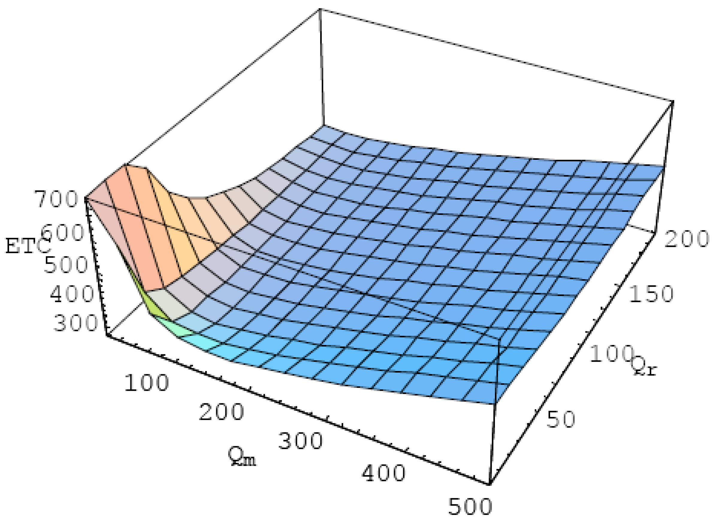
We applied Mathematica5.0 software to bring the numerical examples into the formula, and used the Find minimum command to find the best order batch Q_m and the best recycling remanufacturing batch Q_r, then took the integer value, using the rounding method, to calculate the minimum total cost per unit time. The recovery rate γ is random, γ = 1/λ, and γ < λ, λ follows the exponential distribution, and we know that γ > 1/λ.

The data of this research example are: the demand per unit time λ is 10, the average recovery per unit time γ is 8, the manufacturing center’s order cost per unit time is 200, the manufacturing center’s inventory holding cost per unit time is 1, the manufacturing center’s purchase cost per unit time is 10, and the recycling processing center’s setup cost per unit time is 500. The inventory holding cost per unit time of the recycling processing center is 1, and the cost per unit time of the recycling processing center is 10.

Bringing the aforementioned data into the formula, the best order batch size of the manufacturing center is 99, the best manufacturing batch size of the recycling processing center is 59, and the best total cost is 306.321. It is divided into 3D graphics as shown in Figure 10.

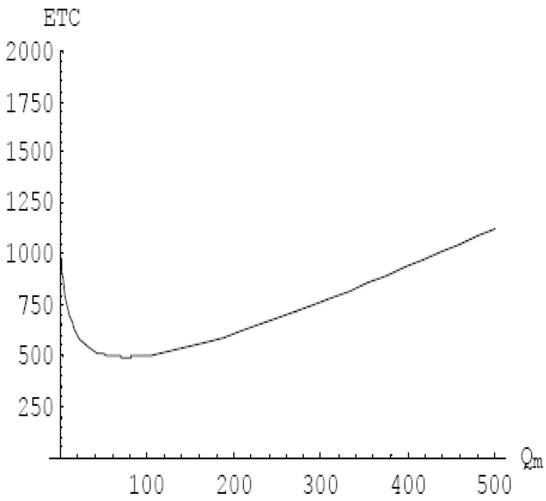
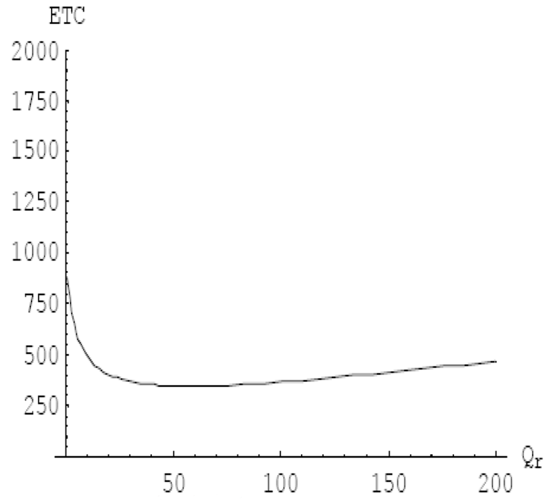
For the analysis of Q_m and Q_r, when the remanufacturing batch Q_r of the recycling processing center is 10, the order batch, Q_m, is 75 and the minimum ETC value is 494.603. We can see the changes in Qm and ETC in Figure 10. Conversely, when the manufacturing center’s order batch Q_m is set to 80, the remanufacturing batch, Qr, is 58 and the minimum ETC value is 348.07. The changes in Q_m and ETC can be seen in Figure 11 and Figure 12.

From the above solution, it shows that the inventory strategies proposed by this study can reach the minimum total cost per unit time, the best order batch of the manufacturing center and the best remanufacturing batch of the recycling processing center.

5. Conclusions

The method presented in this article is to use the Fuzzy Set method to determine the main impact on the recovery process and its corresponding weight, then use AHP to determine the relationship between the recovery and processing levels. The GDSS system has also been developed to support such measurement methods and procedures. The method proposed in this article is compared with the GDSS system that promotes recycling. It also provides a convenient way for recyclers or manufacturers to sort their own products and use fuzzy numbers to select a set of test standards. In the operation description section of the fuzzy set, this article uses the variable code in the formula to investigate the recycler’s product level. In the evaluation process of this method, there are still some errors in the evaluation from the recycling processor, but if there are more experts to evaluate and define, the classification criteria will be clearer, and the recovery processing situation obtained will be more accurate.

We integrate the inventory control model at the recovery process level. Although the analysis model is quite accurate, the higher the recovery rate is, the more difficult the recovery rate and the remanufacturing rate are. It is not easy to determine the related recovery rate; however, we first define and calculate the probability of each recovery process level by the fuzzy theoretical limit, which is conducive to findings that are more in line with the actual inventory model and total cost. Abandonment is still a necessary decision in this study, because the change in the recovery rate will increase the inventory level and the total cost. We find that if the recovery rate is more than 90%, the cost of processing and recovery will be more than doubled. This study also finds the minimum total cost per unit time, the best order batch size of the manufacturing center and the best remanufacturing batch size of the recycling processing center.

Besides, the green circular economy and corporate responsibility awareness are becoming more and more important. In addition to the government’s green supply chain counseling policy, an authentication mechanism for corporate responsibility of upstream and downstream manufacturers for recycling is also required, so that the recycling rate of defective products can reach 100% recycling as soon as possible.

For further study, we suggest that the internal value of the model can be understood from more complex production scenarios, and that government policies for recycling subsidies and good green enterprise certification among manufacturers should be taken into account. The reverse supply chain to recycle and process the recycled products into rebirths should be encouraged, and should induce the final product manufacturers in the forward supply chain to increase the purchase of rebirths, so that the operation of the color supply chain can be more efficient.

References

1. Thierry, M.; Salomon, M.; Van Nunen, J.; Van Wassenhove, L. Strategic issues in product recovery management. Calif. Manag. Rev. 1995, 37, 114–135. [Google Scholar] [CrossRef] [Green Version]
2. Fleischmann, M.; Jacqueline, M.B.-R. Quantitative models for reverse logistics: A review. Eur. J. Oper. Res. 1997, 103, 1–17. [Google Scholar] [CrossRef] [Green Version]
3. Carter, C.R.; Ellram, L.M. Reverse Logistics: A review of the literature and framework for future investigation. J. Bus. Logist. 1998, 19, 85–102. [Google Scholar]
4. Guide, V.D.R.; Van Wassenhove, L. The reverse supply chain. Harv. Bus. Rev. 2002, 80, 25–26. [Google Scholar]
5. Zadeh, L.A. Outline of a new approach to the analysis of complex systems and decision processes. IEEE Trans. Syst. Man Cybern. 1973, 1, 28–44. [Google Scholar] [CrossRef] [Green Version]
6. Jang, J.-Y.R.; Sun, C.-T.; Mizutani, E. Neuro-Fuzzy and Soft Computing: A Computational Approach to Learning and Machine Intelligence; Prentice Hall: New Jersey, NJ, USA, 1996. [Google Scholar]
7. Zipkin, P. Mortgages and Markov chains: A simplified evaluation model. Manag. Sci. 1993, 39, 683–691. [Google Scholar] [CrossRef]
8. Aase, K.K. A Markov model for the pricing of catastrophe insurance futures and spreads. J. Risk Insur. 2001, 68, 25–49. [Google Scholar] [CrossRef]
9. Ching, W.K.; Fung, E.S.; Ng, M.K. A multivariate Markov chain model for categorical data sequences and its applications in demand predictions. IMA J. Manag. Math. 2002, 13, 187–199. [Google Scholar] [CrossRef]
10. Naranjo, L.; Pérez, C.J.; Fuentes-García, R.; Martín, J. A hidden Markov model addressing measurement errors in the response and replicated covariates for continuous nondecreasing processes. Biostatistics 2019, 1–15. [Google Scholar] [CrossRef] [PubMed]
11. Naranjo, L.; Luz, J.; Esparza, R.; Pérez, C.J. A Hidden Markov Model to Address Measurement Errors in Ordinal Response Scale and Non-Decreasing Process. Mathematics 2020, 8, 622. [Google Scholar] [CrossRef] [Green Version]
12. Lin, C.-C.; Lin, C.-W. Defective item inventory model with remanufacturing or replenishing in an integrated supply chain. Int. J. Integr. Supp. Manag. 2011, 6, 254–269. [Google Scholar] [CrossRef]
13. Lin, C.-C.; Su, C.-T. Inventory model for the batch processing of defective products in manufacturing and remanufacturing. Adv. Mater. Res. 2013, 756–759, 4604–4611. [Google Scholar] [CrossRef]
14. Verhoeven, P.; Sinn, F.; Herden, T.T. Examples from Blockchain Implementations in Logistics and Supply Chain Management: Exploring the Mindful Use of a New Technology. Logistics 2018, 2, 20. [Google Scholar] [CrossRef] [Green Version]
15. Ho, T.-F.; Lin, C.-C.; Lin, C.-L. Determining the Optimal Inventory and Number of Shipments for a Two-Resource Supply Chain with Correlated Demands and Remanufacturing Products Allowing Backorder. Mathematics 2020, 8, 548. [Google Scholar] [CrossRef] [Green Version]
16. Minner, S.; Kiesmüller, G.P. Dynamic product acquisition in closed loop supply chains. Int. J. Prod. Res. 2012, 50, 2836–2851. [Google Scholar] [CrossRef] [Green Version]
17. Zhang, X.; Zhao, G.; Qi, Y.; Li, B. A robust fuzzy optimization model for closed-loop supply chain networks considering sustainability. Sustainability 2019, 11, 5726. [Google Scholar] [CrossRef] [Green Version]
18. Govindan, K.; Mina, H.; Esmaeili, A.; Mohamma, S.; Gholami-Zanjani, S.M. An integrated hybrid approach for circular supplier selection and closed loop supply chain network design under uncertainty. J. Clean. Prod. 2020, 242, 1183172. [Google Scholar] [CrossRef]
19. Van der Laan, E.; Dekker, R.; Salomon, M.; Ridder, A. An (s, Q) inventory model with remanufacturing and disposal. Int. J. Prod. Econ. 1996, 46, 339–350. [Google Scholar] [CrossRef] [Green Version]
20. Wiecek, P.; Kubek, D.; Aleksandrowicz, J.; Strózek, A. Framework for onboard bus comfort level predictions using the markov chain concept. Symmetry 2019, 11, 755. [Google Scholar] [CrossRef] [Green Version]
21. Alyousifi, Y.; Othman, M.; Sokkalingam, R.; Faye, I.; Petronio, C.L.S. Predicting daily air pollution index based on fuzzy time series markov chain model. Symmetry 2020, 12, 293. [Google Scholar] [CrossRef] [Green Version]
22. Muckstadt, J.A.; Sapra, A. Principles of Inventory Management: When You Are Down to Four, Order More; Springer: New York, NY, USA, 2010; ISBN 978-0-387-24492-1. [Google Scholar]
Figure 1. Schematic diagram of product production and recycling. (Data source: Thierry M., Salomon M., Van Nunen J., Van Wassenhove L. (1995) [1]).
Symmetry 12 01226 g001
Figure 2. The recycling transfer graph with single-processing level return.
Symmetry 12 01226 g002
Figure 3. The recycling transfer graph with multiple-period returns.
Symmetry 12 01226 g003
Figure 4. Recycling transfer graph with multiple-processing level returns.
Symmetry 12 01226 g004
Figure 5. Recycling transfer graph with multiple-processing levels and multiple-period returns.
Symmetry 12 01226 g005
Figure 6. Triangular fuzzy number graphs.
Symmetry 12 01226 g006
Figure 7. Hyper surface.
Symmetry 12 01226 g007
Figure 8. Graph of change in unit cost of recovery rate.
Symmetry 12 01226 g008
Figure 9. Unit price chart integrating different levels of recovery rates.
Symmetry 12 01226 g009
Figure 10. Manufacturer and remanufacturer order batch change chart.
Symmetry 12 01226 g010
Figure 11. Manufacturers ordering batches total cost change chart.
Symmetry 12 01226 g011
Figure 12. Remanufacturer order batches total cost change chart.
Symmetry 12 01226 g012