Stability Analysis of the Magnetized Casson Nanofluid Propagating through an Exponentially Shrinking/Stretching Plate: Dual Solutions

Abstract

In this research, we intend to develop a dynamical system for the magnetohydrodynamic (MHD) flow of an electrically conducting Casson nanofluid on exponentially shrinking and stretching surfaces, in the presence of a velocity and concertation slip effect, with convective boundary conditions. There are three main objectives of this article, specifically, to discuss the heat characteristics of flow, to find multiple solutions on both surfaces, and to do stability analyses. The main equations of flow are governed by the Brownian motion, the Prandtl number, and the thermophoresis parameters, the Schmid and Biot numbers. The shooting method and three-stage Lobatto IIIa formula have been employed to solve the equations. The ranges of the dual solutions are $f_{wc1}\le f_w$ and ${\lambda }_c\le \lambda$, while the no solution ranges are $f_{wc1}>f_w$ and ${\lambda }_c>\lambda$. The results reveal that the temperature of the fluid increases with the extended values of the thermophoresis parameter, the Brownian motion parameter, and the Hartmann and Biot numbers, for both solutions. The presence of dual solutions depends on the suction parameter. In order to indicate that the first solution is physically relevant and stable, a stability analysis has been performed.

1. Introduction

There are many kinds of non-Newtonian fluids; namely, Casson fluid, Carreau fluid, Williamson fluid, Maxwell fluid, Micropolar fluid, Jeffrey fluid, Second and third-grade fluids, Burgers’ fluid, Eyring–Powell fluid, and so forth [1,2,3,4,5,6,7]. Non-Newtonian fluids are those which are composed of blends. Examples of this type of fluid are pastes, blood, slurries, ketchup, polymer solutions and gels. In simple words, fluids that don’t comply with Newton’s law of viscosity are non-Newtonian fluids, where shear stress is not directly proportional to the gradient of velocity. However, most previous attempts have been made to derive single solutions of non-Newtonian fluids over different surfaces. In the current research, the MHD flow of a non-Newtonian nanofluid in the presence of velocity and concentration slip parameters has been investigated, along with the effect of the convective boundary condition on exponentially stretching and shrinking sheets. It is worth mentioning that the conduct of flow on an exponential sheet is very dissimilar between linear and non-linear sheets. According to Nakamura and Sawada [8], Mustafa, et al. [9] and Nadeem et al. [10], Casson introduced the term Casson fluid in 1959 for the prognostication of the flow conduct of a pigment–oil suspension. This is a kind of non-Newtonian fluid in which the relation to yield and shear stresses are important. When the applied shear stress is less than the yield stress at that momentum, the behavior of the fluid resembles a solid. On the other hand, if the yield stress is not as much as the applied shear stress, then it begins moving. Casson fluid can be described as a shear-thinning fluid that has a zero rate of shear at infinite viscosity, and an infinite rate of shear at zero viscosity; yield stress below these values indicates no occurring flow [11]. Honey, nectar, tomato sauce and jelly are some common examples of Casson fluid. Motivated by the applications and practical significance of the Casson fluids in the fields of food processing, bioengineering, and so on, the key objective of this research is to comprehend the basics of numerous physical parameters and their effects on Casson fluid by employing the mathematical Casson fluid model, proposed by the fundamental work of Casson, in the model of Buongiorno [12] for a nanofluid.

Magnetohydrodynamics, or MHD, is the science of the electrically conducting fluid flow, along with the magnetic field. MHD can be defined accordingly: ‘magneto’ means magnetic, ‘hydro’ means fluids and ‘dynamics’ means motion or movement. Equivalent terms to MHD, that are utilized less as often, are the terms hydromagnetic or magnetofluid dynamics. Ionized gases, like the solar atmosphere, which are commonly called plasmas or fluid metals, like gallium, molten iron and mercury, are fluids. The magnetohydrodynamics field was introduced by a famous Swedish physicist, Hannes Alfvén (1908–1995). For pioneering work and disclosures in MHD with productive applications in various areas of plasma physics, he was awarded the Nobel prize in physics in 1970. The focus of researchers on MHD flow commenced in 1918 after an electromagnetic pump was introduced by Hartmann. There are many useful applications of the non-uniform transverse magnetic field in the various fields of engineering. In the presence of the magnetic field, electrically conducting fluids flow has significant applications, for example, cooling nuclear reactors, oil exploration, magnetohydrodynamic generators, plasma studies and geothermal energy extraction [13,14,15,16,17,18,19]. The flow of MHD had been taken into account by numerous scholars in their studies because of its important usages, some examples being William [20,21], Eastman et al. [22] and Hossain [23]. Recent work on the MHD boundary layer flow of a Casson nanofluid with different slip boundary conditions can be seen in these articles [24,25,26]. All the above studies have been performed on single solutions only. We tried to find all possible multiple solutions and dual solutions in this study.

The concept of boundary axisymmetric flow, on a continuously stretched sheet with a fixed velocity, was introduced by Sakiadis [27]. Since then, numerous works on the flow of the boundary layer on a stretched surface have been undertaken due to their vast applicability in industry, for instance, in materials manufactured by extrusion, the manufacture of rubber and plastic sheets, hot rolling, the production of glass fiber, the cooling of a large metal plate in a bath, the production of paper and the extrusion of polymer sheets. The exact analytical solution of the boundary layer flow over a stretching surface was first found by Crane [28]. Gupta and Gupta [29] considered the viscous fluid flow, with a concentration effect, on a stretched sheet. The important characteristics of the transfer of heat were investigated by Grubka and Bobba [30] by considering the flow on the stretched surface. An unsteady flow on the stretched surface has been studied by Andersson et al. [31]. The nanofluid flow over a stretching flat sheet, incorporating the effects of thermophoresis and the Brownian motion parameters, was first studied by Khan and Pop [32]. Due to the importance of both surfaces, we attempt to get results for both surfaces; however, more results have been taken into account for the shrinking surface, because a huge number of researchers consider stretching surfaces in their studies. It is our expectation that these mathematical results will provide help for other researchers who are working on nanofluids and in nano-technology fields via an experimental approach.

2. Mathematical Formulation

The flow of an electrically conducting two-dimensional (2D) Casson nanofluid on exponentially shrinking and stretching surfaces is assumed. The state rheological equations for the isotropics of Casson fluid are expressed as [8,9,10]

$${\tau }_{ij}=\{\begin{array}{l}\left({\mu }_B+\left(\frac{P_y}{\sqrt{2\pi }}\right)\right)2e_{ij}, \pi >{\pi }_c \\ \left({\mu }_B+\left(\frac{P_y}{\sqrt{2{\pi }_c}}\right)\right)2e_{ij}, \pi <{\pi }_c \end{array}$$

(1)

where $P_y,{\mu }_B$ are the yield stress and plastic dynamic viscosity of Casson fluid, respectively. Moreover, ${\pi }_c$ is a critical value of $\pi$ based on the non-Newtonian model, and $e_{ij}$ is the (i, j)th component of the deformation rate, expressed as π = $e_{ij}{e}_{ij}$. The surface velocity is presumed as $u_w=\lambda a{e}^{\raisebox{1ex}{$x$}\!\left/ \!\raisebox{-1ex}{$l$}\right.}$, where $a$ is the characteristic velocity of the surface and $\lambda <0$ and $\lambda >0$ indicate the shrinking and stretching surface, respectively. Further, we supposed that the variable magnetic field has a strength of $B=B_0{e}^{\raisebox{1ex}{$x$}\!\left/ \!\raisebox{-1ex}{$2l$}\right.}$, where $B_0$ is the constant magnetic field. The induced magnetic field is neglected by assuming the number of low magnetic Reynolds.

The field of the velocity of the boundary layers of the Casson nanofluid’s flow, with temperature and concentration equations, can be expressed as

$$\frac{\partial u}{\partial x}+\frac{\partial v}{\partial y}=0$$

(2)

$$u\frac{\partial u}{\partial x}+v\frac{\partial u}{\partial y}=\vartheta \left(1+\frac{1}{\beta }\right)\frac{{\partial }^{2}u}{\partial y^2}-\frac{{\sigma }^{*}{B}^{2}u}{\rho }$$

(3)

$$u\frac{\partial T}{\partial x}+v\frac{\partial T}{\partial y}=\alpha \frac{{\partial }^{2}T}{\partial y^2}+{\tau }_w \left[D_B \frac{\partial C}{\partial y} \frac{\partial T}{\partial y}+\frac{D_T}{T_{\infty }} {\left(\frac{\partial T}{\partial y}\right)}^2\right]$$

(4)

$$u \frac{\partial C}{\partial x}+v \frac{\partial C}{\partial y}=D_B \frac{{\partial }^{2}C}{\partial y^2}+\frac{D_T}{T_{\infty }} \frac{{\partial }^{2}T}{\partial y^2}$$

(5)

The related boundary conditions (2–5) are

$$\begin{gathered} v=v_w , u=u_w+A^{*}\vartheta \left(1+\frac{1}{\beta }\right)\frac{\partial u}{\partial y},-k_f \frac{\partial T}{\partial y}=h_f\left(T_f-T\right), C=C_w+N\frac{\partial C}{\partial y} at y=0 \\ u\to 0, T \to T_{\infty }, C\to C_{\infty } as y\to \infty \end{gathered}$$

(6)

where $u$ is the velocity component along the $x$-axis, $v$ is the velocity component along the $y$-axis, $\vartheta ,\beta =\frac{{\mu }_B\sqrt{2\pi }}{P_y},\rho ,{\sigma }^{*}, \alpha , D_B, D_T$ are the viscosity of the fluid, the Casson parameter, the density of fluid, the electrical conductivity, the thermal diffusivity, the Brownian motion and the thermophoresis, respectively. ${\tau }_w$ is the heat capacity of the nanofluid and the effective heat capacity of the nanoparticle material, and $T_{\infty }$ and $C_{\infty }$ are ambient temperature and concentration correspondingly, such that $T_f>T_{\infty }$ and $C_w>C_{\infty }$. $A^{*}=A_1^{*}{e}^{\raisebox{1ex}{$-x$}\!\left/ \!\raisebox{-1ex}{$2l$}\right.}$ is the velocity condition, where $A_1^{*}$ is the slip factor of velocity, and $N=N_1{e}^{\raisebox{1ex}{$-x$}\!\left/ \!\raisebox{-1ex}{$2l$}\right.}$ is the concentration condition where $N_1$ is the slip factor of concentration.

We will employ similar variables (7) in Equations (2)–(6) in order to obtain similar solutions.

$$\psi =\sqrt{2\vartheta la}{e}^{\raisebox{1ex}{$x$}\!\left/ \!\raisebox{-1ex}{$2l$}\right.}f\left(\eta \right) , \theta \left(\eta \right)=\frac{\left(T-T_{\infty }\right)}{\left(T_f-T_{\infty }\right)}, \varnothing \left(\eta \right)=\frac{\left(C-C_{\infty }\right)}{\left(C_w-C_{\infty }\right)}, \eta =y\sqrt{\frac{a}{2\vartheta l}} e^{\raisebox{1ex}{$x$}\!\left/ \!\raisebox{-1ex}{$2l$}\right.}$$

(7)

where the stream function has the following relations with the velocity components $u=\frac{\partial \psi }{\partial y} , v=-\frac{\partial \psi }{\partial x}$.

By substitution of the stream function relations with Equation (7) in (2)–(6), we obtain

$$\left(1+\frac{1}{\beta }\right)f^{‴}+f{f}^{″}-2f^{\prime 2}-M=0$$

(8)

$$\frac{1}{Pr}{\theta }^{″}+f{\theta }^{\prime }+N_b{\varnothing }^{\prime }{\theta }^{\prime }+N_t{\left({\theta }^{\prime }\right)}^2=0$$

(9)

$${\varnothing }^{″}+Scf{\varnothing }^{\prime }+\frac{N_t}{N_b}{\theta }^{″}=0$$

(10)

along with the boundary conditions

$$\begin{gathered} f\left(0\right)=f_w, f^{\prime }\left(0\right)=\lambda +\delta \left(1+\frac{1}{\beta }\right)f^{″}\left(0\right), {\theta }^{\prime }\left(0\right)=-A\left[1-\theta \left(0\right)\right], \\ \varnothing \left(0\right)=1+{\delta }_C{\varnothing }^{\prime }\left(0\right), f^{\prime }\left(\eta \right) \to 0, \theta \left(\eta \right)\to 0, \varnothing \left(\eta \right)\to 0 as \eta \to \infty \end{gathered}$$

(11)

Here, prime denotes the derivative with respect to $\eta$, $M=\frac{2l{\sigma }^{*}{\left(B_0\right)}^2}{\rho a}$ is the magnetic field, $Pr=\frac{\vartheta }{\alpha }$ is the Prandtl number, and $N_t=\frac{{\tau }_1{D}_T\left(T_f-T_{\infty }\right)}{\vartheta T_{\infty }}$ and $N_b=\frac{{\tau }_1{D}_B\left(C_w-C_{\infty }\right)}{\vartheta }$ are the thermophoresis and Brownian motion parameters, respectively. Furthermore, $Sc=\frac{\vartheta }{D_B}$ denotes the Schmidt number, $\lambda$ is the stretching/shrinking parameter, $v_w=-\sqrt{\frac{\vartheta a}{2l}}{e}^{\raisebox{1ex}{$x$}\!\left/ \!\raisebox{-1ex}{$2l$}\right.}{f}_w$ is the suction/blowing parameter, $\delta =A_1^{*}\sqrt{\frac{\vartheta a}{2l}}$ is the velocity slip parameter, ${\delta }_C=N_1\sqrt{\frac{a}{2\vartheta l}}$ is the concentration slip parameter, and the Biot number or convective parameter is $A=\frac{h_f}{k_f}\sqrt{\frac{2\vartheta l}{a}}{e}^{\raisebox{1ex}{$-x$}\!\left/ \!\raisebox{-1ex}{$2l$}\right.}$, where $h_f=U_0{e}^{\raisebox{1ex}{$x$}\!\left/ \!\raisebox{-1ex}{$2l$}\right.}$ ($U_0$ is a constant), which implies that $A=\frac{U_0}{k_f}\sqrt{\frac{2\vartheta l}{a}}$.

As regards the coefficient of skin friction, the local Nusselt and Sherwood numbers are physical quantities of interest, and can be defined as follows

$$\begin{gathered} C_f=\frac{{\left[\mu \left(1+\frac{1}{\beta }\right)\frac{\partial u}{\partial y}\right]}_{y=0}}{\rho a^2}, N_u=\frac{-x{\left(\frac{\partial T}{\partial y}\right)}_{y=0}}{\left(T_f-T_{\infty }\right)}, S_h=\frac{-x{\left(\frac{\partial C}{\partial y}\right)}_{y=0}}{\left(C_w-C_{\infty }\right)} \\ {C}_f{\left(R{e}_x\right)}^{\frac{1}{2}}=\left(1+\frac{1}{\beta }\right)f^{″}\left(0\right), N_u{\left(R{e}_x\right)}^{-\frac{1}{2}}=-{\theta }^{\prime }\left(0\right), S_h{\left(R{e}_x\right)}^{-\frac{1}{2}}=-{\varnothing }^{\prime }\left(0\right) \end{gathered}$$

(12)

where $R{e}_x=\frac{ax}{\vartheta }$ is the Reynold number.

3. Stability Analysis

Weidman et al. [33] proposed stability solutions, and Haris and Pop [34] proceeded with them in their studies, wherein multiple solutions for the boundary layer have been considered. From their work, it is determined that the additional solution is unrealizable, and said to be an unstable solution. On the other hand, the first solution is the physically realizable solution, which is said to be a stable solution. The initial step of obtaining the stable solution is to change Equations (2)–(5) to the unsteady governing equations, by presenting a new dimensionless variable, $\tau =\frac{a}{2l}{e}^{\raisebox{1ex}{$x$}\!\left/ \!\raisebox{-1ex}{$l$}\right.}.t$, as suggested by Merkin [35]. Thus, we have

$$\frac{\partial u}{\partial t}+u \frac{\partial u}{\partial x}+v \frac{\partial u}{\partial y}=\vartheta \left(1+\frac{1}{\beta }\right) \frac{{\partial }^{2}u}{\partial y^2}-\frac{{\sigma }^{*} B^2 u}{\rho }$$

(13)

$$\frac{\partial T}{\partial t}+u \frac{\partial T}{\partial x}+v \frac{\partial T}{\partial y}=\alpha \frac{{\partial }^{2}T}{\partial y^2}+{\tau }_w \left[D_B \frac{\partial C}{\partial y} \frac{\partial T}{\partial y}+\frac{D_T}{T_{\infty }} {\left(\frac{\partial T}{\partial y}\right)}^2\right]$$

(14)

$$\frac{\partial C}{\partial t}+u \frac{\partial C}{\partial x}+v \frac{\partial C}{\partial y}=D_B \frac{{\partial }^{2}C}{\partial y^2}+\frac{D_T}{T_{\infty }} \frac{{\partial }^{2}T}{\partial y^2}$$

(15)

It is interesting to highlight that the presence of $\tau$ is associated with initial value problems, which correspond to the stable solution. After the integration of $\tau =\frac{a}{2l}{e}^{\raisebox{1ex}{$x$}\!\left/ \!\raisebox{-1ex}{$l$}\right.}.t$ with $\eta =y\sqrt{\frac{a}{2\vartheta l}} e^{\raisebox{1ex}{$x$}\!\left/ \!\raisebox{-1ex}{$2l$}\right.}$, we have following new similarity transformation variables

$$\psi =\sqrt{2\vartheta la}{e}^{\raisebox{1ex}{$x$}\!\left/ \!\raisebox{-1ex}{$2l$}\right.}f\left(\eta ,\tau \right), \theta \left(\eta ,\tau \right)=\raisebox{1ex}{$\left(T-T_{\infty }\right)$}\!\left/ \!\raisebox{-1ex}{$\left(T_f-T_{\infty }\right)$}\right., \varnothing \left(\eta ,\tau \right)=\raisebox{1ex}{$\left(C-C_{\infty }\right)$}\!\left/ \!\raisebox{-1ex}{$\left(C_w-C_{\infty }\right)$}\right.$$

(16)

Replacing Equations (13)–(15) with Equation (16), we obtain

$$\left(1+\frac{1}{\beta }\right)f_{\eta \eta \eta }+f{f}_{\eta \eta }-2{\left(f_{\eta }\right)}^2-M{f}_{\eta }-f_{\eta \tau }=\tau \left(f_{\eta }{f}_{\eta \tau }-f_{\eta \eta }{f}_{\tau }\right)$$

(17)

$$\frac{1}{Pr}{\theta }_{\eta \eta }+f{\theta }_{\eta }+N_b{\theta }_{\eta }{\varnothing }_{\eta }+N_t{\left({\theta }_{\eta }\right)}^2-{\theta }_{\tau }=2\left(f_{\eta }{\theta }_{\tau }-{\theta }_{\eta }{f}_{\tau }\right)$$

(18)

$${\varnothing }_{\eta \eta }+Scf{\varnothing }_{\eta }+\frac{N_t}{N_b}{\theta }_{\eta \eta }-Sc{\varnothing }_{\tau }=2.Sc.\tau .\left(f_{\eta }{\varnothing }_{\tau }-{\varnothing }_{\eta }{f}_{\tau }\right)$$

(19)

subject to the boundary conditions

$$\begin{gathered} f\left(0,\tau \right)=f_w, \frac{\partial f\left(0, \tau \right)}{\partial \eta }=\lambda +\delta \left(1+\frac{1}{\beta }\right)\frac{{\partial }^{2}f\left(0, \tau \right)}{\partial {\eta }^2}, \mathrm{and}\frac{\partial f\left(\eta , \tau \right)}{\partial \eta } \to 0 as \eta \to \infty \\ \frac{\partial \theta \left(0, \tau \right)}{\partial \eta }=-A\left[1-\theta \left(0,\tau \right)\right] \mathrm{and} \theta \left(\eta ,\tau \right) \to 0 as \eta \to \infty \\ \varnothing \left(0,\tau \right)=1+{\delta }_C\frac{\partial \varnothing \left(0, \tau \right)}{\partial \eta } \mathrm{and} \varnothing \left(\eta ,\tau \right)\to 0 as \eta \to \infty \end{gathered}$$

(20)

Subsequently, to classify the stability of the solution $f\left(\eta \right)=f_0\left(\eta \right),\theta \left(\eta \right)={\theta }_0\left(\eta \right)$ and $\varnothing \left(\eta \right)={\varnothing }_0\left(\eta \right)$, which solved the boundary value problems of Equations (17)–(20), we will follow the steps of Rosca and Pop [36];

$$\begin{array}{c}f\left(\eta ,\tau \right)=f_0\left(\eta \right)+e^{-\epsilon \tau }F\left(\eta ,\tau \right)\\ \theta \left(\eta ,\tau \right)={\theta }_0\left(\eta \right)+e^{-\epsilon \tau }G\left(\eta ,\tau \right)\\ \varnothing \left(\eta ,\tau \right)={\varnothing }_0\left(\eta \right)+e^{-\epsilon \tau }H\left(\eta ,\tau \right)\end{array}$$

(21)

where $F\left(\eta ,\tau \right), G\left(\eta ,\tau \right)$ and $H\left(\eta ,\tau \right)$ are corresponding small relatives of $f_0\left(\eta \right)$,${\theta }_0\left(\eta \right)$ and ${\varnothing }_0\left(\eta \right)$, and $\epsilon$ is the unknown eigenvalue parameter which must be found.

By applying Equation (21) in Equations (17)–(19), including boundary condition (20) and keeping the value of $\tau =0$, as recommended in paper [33] to compute the initial decay and growth of the solutions of (21), the functions $F\left(\eta ,\tau \right)$, $G\left(\eta ,\tau \right)$ and $H\left(\eta ,\tau \right)$ are expressed as $F_0\left(\eta \right)$, $G_0\left(\eta \right)$ and $H_0\left(\eta \right)$, respectively. It should be noted that these functions’ ranges must be $0<F\left(\eta ,\tau \right)<1$, $0<G\left(\eta ,\tau \right)<1$ and $0<H\left(\eta ,\tau \right)<1$. Henceforth, we have a system for the linearized eigenvalue problem.

$$\left(1+\frac{1}{\beta }\right)F_0^{‴}+f_0{F}_0^{″}+F_0{f}_0^{″}-4f_0^{\prime }{F}_0^{\prime }-M{F}_0^{\prime }+\epsilon F_0^{\prime }=0$$

(22)

$$\frac{1}{Pr}{G}_0^{″}+f_0{G}_0^{\prime }+F_0{\theta }_0^{\prime }+N_b{\varnothing }_0^{\prime }{G}_0^{\prime }+N_b{H}_0^{\prime }{\theta }_0^{\prime }+2N_t{\theta }_0^{\prime }{G}_0^{\prime }+\epsilon G_0=0$$

(23)

$$H_0^{″}+Sc\left(f_0{\varnothing }_0^{\prime }+F_0{H}_0^{\prime }\right)+\frac{N_t}{N_b}{G}_0^{″}+Sc\epsilon H_0=0$$

(24)

with the boundary condition

$$\begin{array}{c}{F}_0\left(0\right)=0, F_0^{\prime }\left(0\right)=\delta \left(1+\frac{1}{\beta }\right)F_0^{″}\left(0\right), \mathrm{and} F_0^{\prime }\left(\eta \right)\to 0 as \eta \to \infty \\ A{G}_0\left(0\right)=G_0^{\prime }\left(0\right) \mathrm{and} G_0\left(\eta \right)\to 0 as \eta \to \infty \\ H_0\left(0\right)={\delta }_C{H}_0^{\prime }\left(0\right) \mathrm{and} H_0\left(\eta \right)\to 0 as \eta \to \infty \end{array}$$

(25)

According to the previous study of Haris et al. [34], in order to find the smallest possible eigenvalues, we need to relax one boundary condition of the functions $F_0\left(\eta \right)$, $G_0\left(\eta \right)$ and $H_0\left(\eta \right)$. In the current problem, we relaxed the $F_0^{\prime }\left(\eta \right)\to 0$ as $\eta \to \infty$, and then solved the Equations (22)–(25) with the new relaxed initial conditions $F_0^{″}\left(0\right)=1$. It is worth mentioning that if the value of $\epsilon >0$, then the initial decay of disturbances exists, and the flow becomes stable and physically realizable. Further, if the value of $\epsilon <0$, this indicates the initial growth of disturbances in the system, and the flow becomes unstable.

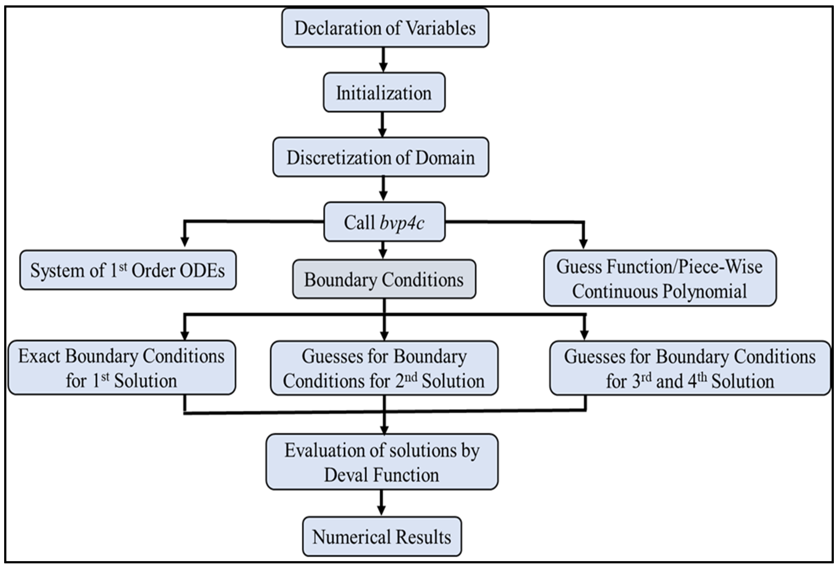
4. Numerical Methods

In this section, the numerical procedures of the shooting method and the three-stage Lobatto IIIa formula are described. These methods are very simple and highly accurate in computing results for the boundary layer flow problems, and many researchers use them to obtain multiple solutions and the stability analyses of the solutions.

4.1. Shooting Method

The shooting method is an iterative method that changes the boundary value problems (BVPs) into equivalent the initial value problems (IVPs) by using a sequence of initial condition guesses, obtained using an appropriate iterative method, until the required accuracy is reached. The resultant IVPs are then solved by employing the suitable IVP method presented in the literature. In this problem, we have used the well-known Runge–Kutta method of the fourth order, which is known because of its high accuracy. The descriptions of the method are as follows

$$p=f^{\prime },q=p^{\prime }; \left(1+\frac{1}{\beta }\right)q^{\prime }=2p^2-fq+MP$$

(26)

$$r={\theta }^{\prime }; r^{\prime }=Pr\left\{-fr-N_{b}s.r-N_t{r}^2\right\}$$

(27)

$$s={\varphi }^{\prime }; s^{\prime }=-Scfs-\frac{N_t}{N_b} r^{\prime }$$

(28)

with conditions

$$\{\begin{array}{c}f\left(0\right)=f_w, p\left(0\right)=\lambda +\delta \left(1+\frac{1}{\beta }\right){\alpha }_1, \mathrm{and} q\left(0\right)={\alpha }_1\\ {\alpha }_2=-A\left[1-\theta \left(0\right)\right]\mathrm{and} r\left(0\right)={\alpha }_2\\ \varphi \left(0\right)=1+{\delta }_C{\alpha }_3 \mathrm{and} s\left(0\right)={\alpha }_3\end{array}$$

(29)

where the unknown initial conditions are denoted by ${\alpha }_1$, ${\alpha }_2$ and ${\alpha }_3$. It is worth mentioning that the missing initial values of ${\alpha }_1$, ${\alpha }_2$ and ${\alpha }_3$ are needed to shoot such that the profiles of the solutions satisfy the original boundary conditions, which are $f^{\prime }\left(\eta \right)\to 0, \theta \left(\eta \right)\to 0,\mathrm{and} \varnothing \left(\eta \right)\to 0 \mathrm{as} \eta \to \infty$.

4.2. Three-Stage Lobatto IIIA Formula

This is a well-known numerical method. All types of linear and non-linear differential equations are solved by this method easily. The three-stage Lobatto IIIa formula is created in bvp4c with the help of a finite difference code. Afterward, stability analysis is performed using the bvp4c solver function. According to Rehman et al., [37] “this collocation formula and the collocation polynomial provides a $C_1$ continuous solution that is fourth-order accurate uniformly in $\left[a , b\right]$. Mesh selection and error control are based on the residual of the continuous solution”. Further, the tolerance of the relative error is fixed at ${10}^{-5}$. The suitable mesh determination is created and returned in the field sol.x. The bvp4c returns the solution, called sol.y., as a construction. In any case, values of the solution are gotten from the array named sol.y, relating to the field sol.x. The general procedure of this method, along with stability analysis, is presented in Figure 1.

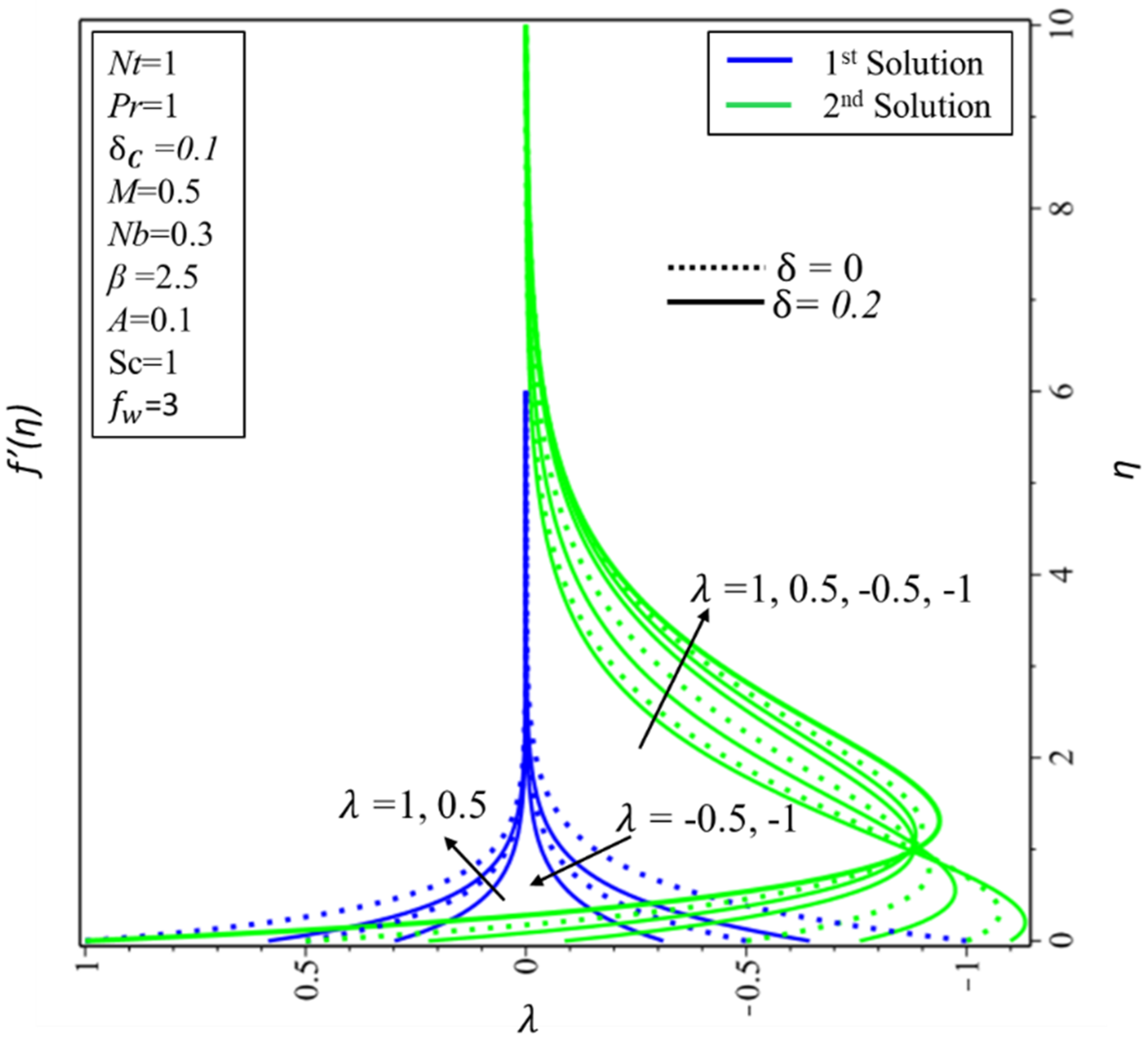
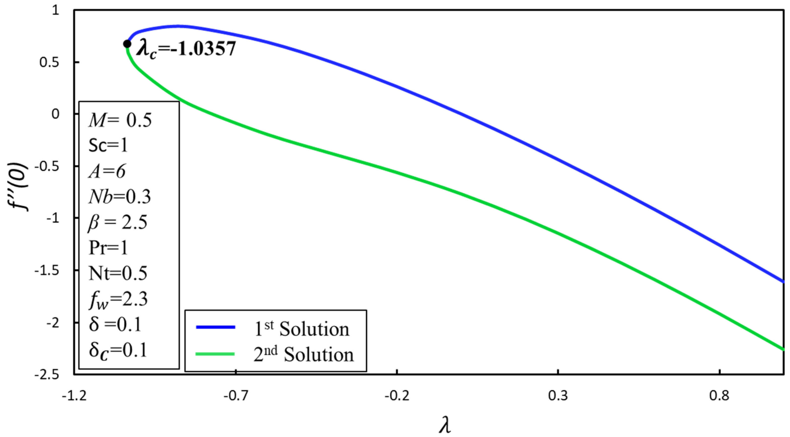
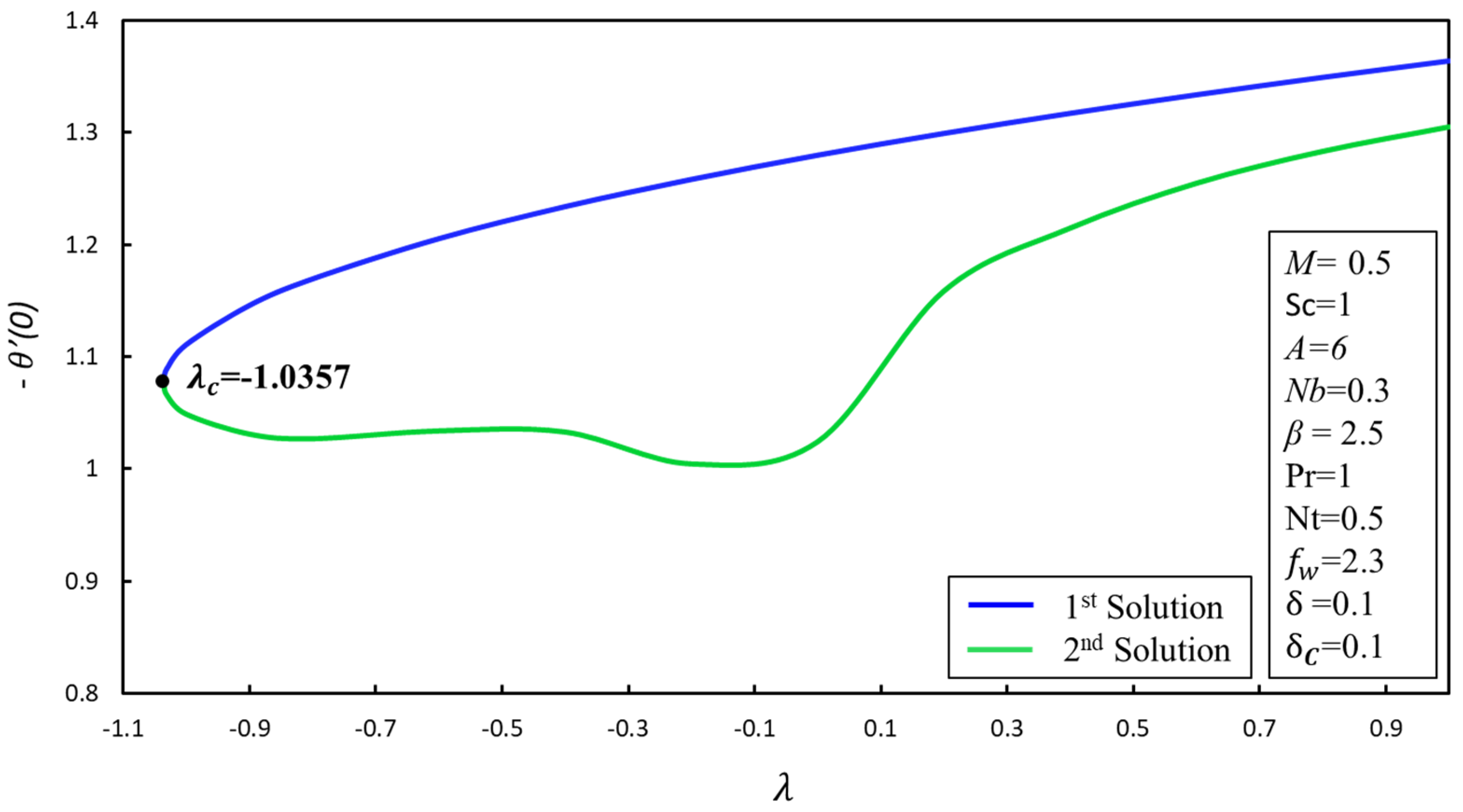
5. Result and Discussion

Providing clear comprehension of the present problem, we performed numerical computation using two numerical methods; specifically, the shooting technique along with the Runge–Kutta method of the fourth order in MAPLE software, and the three-stage Lobatto IIIa formula in bvp4c by employing the finite difference code in MATLAB software. We attempted to plot all the graphs of skin friction ($f^{″}\left(0\right)$), heat ($-{\theta }^{\prime }\left(0\right)$) and concentration ($-{\varnothing }^{\prime }\left(0\right)$) transfer rates, and the temperature, velocity and concentration profiles for numerous values of directly involved parameters, such as the Casson $\left(\beta \right)$ and magnetic parameters $\left(M\right)$, the Schmidt $\left(Sc\right)$ and Prandtl $\left(Pr\right)$ numbers, the thermophoresis $\left(N_t\right)$ and Brownian motion $\left(N_b\right)$ parameters, the suction $\left(f_w\right)$ and velocity slip $\left(\delta \right)$ parameters, and the convection parameter $\left(A\right)$ and concentration slip parameter $\left({\delta }_C\right)$. To validate the correctness of the shooting method, the values of $f^{″}\left(0\right),-{\theta }^{\prime }\left(0\right)$ and $-{\varnothing }^{\prime }\left(0\right)$ are compared with those derived by Rehman et al. [37] and Mustafa et al. [38] in

Table 1. Compression of $-f^{″}\left(0\right)$, $-{\theta }^{\prime }\left(0\right)$ and $-{\varnothing }^{\prime }\left(0\right)$.

${\mathit{N}}_{\mathit{t}}$		[38] ${\mathit{N}}_{\mathit{b}}=0.1$			[37] ${\mathit{N}}_{\mathit{b}}=0.1$			Present Results ${\mathit{N}}_{\mathit{b}}=0.1$
	$-{\mathit{f}}^{″}\left(0\right)$	$-{\mathit{\theta }}^{\prime }\left(0\right)$	$-{\varnothing }^{\prime }\left(0\right)$	$-{\mathit{f}}^{″}\left(0\right)$	$-{\mathit{\theta }}^{\prime }\left(0\right)$	$-{\varnothing }^{\prime }\left(0\right)$	$-{\mathit{f}}^{″}\left(0\right)$	$-{\mathit{\theta }}^{\prime }\left(0\right)$	$-{\varnothing }^{\prime }\left(0\right)$
0.1	1.28181	0.25374	0.37525	1.28180857	0.25373483	0.37525393	1.28180857	0.25373483	0.37525393
0.2	1.28181	0.25192	0.20423	1.28180857	0.25191722	0.20422841	1.28180857	0.25191726	0.20422841
0.3	1.28181	0.25008	0.03662	1.28180857	0.25007701	0.03660736	1.28180857	0.25007701	0.03660735
0.4	1.28181	0.24821	−0.12757	1.28180857	0.24821431	−0.12757046	1.28180857	0.24821430	−0.12757045
0.5	1.28181	0.24633	−0.28826	1.28180857	0.24632922	−0.28826784	1.28180857	0.24632921	−0.28826784

, and we establish excellent concurrences with them; henceforth, we can use the present code confidently. The system of highly non-linear ordinary differential equations (ODEs) (8–10) subject to boundary condition (11) is solved by employing the shooting method with the Runge Kutta (RK)-4th order method in MAPLE software. The shooting technique is an iterative method which changes BVPs into equivalent IVPs by using a sequence of initial condition guesses, obtained using an appropriate iterative method until the required accuracy is reached, and then solved by the shooting technique. This is the accepted method for solving the boundary value problems of ODEs. We kept the minimum and maximum range of ${\eta }_{\infty }=6$ and ${\eta }_{\infty }=10$, respectively, which satisfied the hydrodynamic, temperature and concentration boundary layers asymptotically.

It is worth mentioning that the solution to this problem is the local similar solution. Figure 2 is drawn to show the presence of two solutions in both surfaces, namely the shrinking and stretching surfaces. Figure 3, Figure 4 and Figure 5 show the effect of $\lambda$ on the shear stress $f^{″}\left(0\right)$, the local heat flux $-{\theta }^{\prime }\left(0\right)$ and the local mass flux $-{\varnothing }^{\prime }\left(0\right)$. From these figures, it can be concluded that two sorts of solutions exist; explicitly dual solutions $\left({\lambda }_c\le \lambda \right)$ and no solution $\left({\lambda }_c>\lambda \right)$. It has been observed that the skin friction coefficient is higher for the shrinking surface as compared to the stretching surface in both solutions (refer Figure 3). Further, the behaviors of the heat and concentration transfer seem the same, where $-{\theta }^{\prime }\left(0\right)$ and $-{\varnothing }^{\prime }\left(0\right)$ increase over the stretching surface, as compared to the shrinking surface in the first solution. On the other hand, dual behaviors are noticed in the second solution. The impact of the Casson parameter $\left(\beta \right)$ on the shear stress with various values of the suction parameter $\left(f_w\right)$ is drawn in Figure 6. From studies of Miklavčič and Wang [39], Fang and Zhang [40] and Bhattacharyya [41], it can be concluded that “flow due to the exponentially shrinking surface needs more suction when contrasted with the flow over a linearly shrinking surface so as to keep the larger amount of vorticity produced inside the boundary layer”. For the case of a Newtonian fluid, $\beta =\infty$, the range of dual solution is $f_{wc1}\le f_w$, and the no solution range is $f_{wc1}>f_w$. For Casson fluid cases, multiple solutions rely upon the values of the Casson parameter; for example, high suction is expected to keep up the flow inside the boundary layer for small values of the Casson parameter, as shown in Figure 6. On the other hand, the Casson parameter is relative to the shear stress for the first solution, where the coefficient of skin friction rises when $\beta$ diminishes. For the second solution, the reverse trend was noticed. Figure 7 and Figure 8 display the impact of $\beta$ on local Nusselt and Sherwood numbers separately. The local Nusselt and Sherwood numbers are higher for the greater value of $\beta$, contrasted with a smaller one, which is because we have $\frac{1}{\beta }$ in the momentum equation.

The impact of $\beta$ on the velocity profile appears in Figure 9. The momentum of the boundary layer improves the first solution when $\frac{1}{\beta }$ changes in the absence or the presence of the magnetic parameter. On the other hand, the double nature of the velocity distribution and its boundary layer thickness is noticed in the second solution case when $\beta$ rots; physically, this tends to be explained by the fact that decreases in $\beta$ are caused in order to produce greater viscosity, and as a result resistance is produced in the flow of fluid. Consequently, the hydrodynamic boundary layer becomes thinner. Figure 10 exhibits the impact of $M$ on the velocity distribution with and without the velocity slip effect. The slip effect reduces the velocity boundary layer monotonically in both solutions, when contrasted with $\delta =0$. The momentum boundary layer ends up slenderer in the first solution, and the physical magnetic parameter creates progressively more resistance in the flow of the fluid due to the moving electric charges in nanofluid, and thus the velocity of the fluid deaccelerated. On the other hand, the opposite pattern is perceived for the second solution. Figure 11 demonstrates the effect of the Casson parameter $\left(\beta \right)$ on temperature distribution. The reduction in $\beta$ produces a contrary force in the flow of fluid due to the high viscosity in the fluid flow, thus the temperature of the fluid and the thermal boundary layer thickness decrease continually when $\beta$ declines in both solutions. Figure 12 presents the effect of different Prandtl numbers on the distribution of temperature. The higher convectional number $\left(A\right)$ improves the temperature of the surface and the boundary layer becomes thicker in both solutions, as expected. It is worth noting that $A\to \infty$ indicates the constant temperature of the wall. Further, we know the Prandtl number $\left(Pr\right)$ is the ratio of momentum diffusivity to thermal diffusivity, which implies an enhancement in $Pr$ is the cause of the flimsier thermal diffusivity, and therefore the thickness of the thermal boundary layer becomes thinner, as found in Figure 12. The impact of the Brownian motion $\left(N_b\right)$ and thermophoresis $\left(N_t\right)$ parameters on the temperature profile is exhibited in Figure 13 and Figure 14, respectively. The thicker thermal boundary layer is present as the Brownian motion and thermophoresis parameters rise in all the solutions. Practically, thermophoresis and the Brownian motion help the nanoparticles to change their places from hot to cold regions; in this manner, the thickness of the thermal boundary layer is enhanced monotonically. Figure 15 and Figure 16 reveal the impact of $N_t$ and $N_b$ on concentration distributions. The concentration profile causes a decline in the Brownian motion parameter $\left(N_b\right)$, which is improved in both solutions (refer to Figure 15). On the contrary, the thermophoresis parameter $\left(N_t\right)$ is provably relative to the concentration profile. It is additionally seen that the effect of the concentration slip $\left({\delta }_C\right)$ is the reason for the development of the concentration boundary layer in both solutions (alluded to in Figure 15 and Figure 16). The concentration profile for numerous values of the Schmidt number $\left(Sc\right)$ is drawn in Figure 17. Lower molecular diffusivity is found for a higher Schmidt number $\left(Sc\right)$. Henceforth, a thicker concentration boundary layer in both solutions is possible with the lower values of the Schmidt number $\left(Sc\right)$.

In this study, to measure the stability of the solution, stability analyses are performed. The fact behind this investigation is that if there occurs more than one solution in any problem. The main objective of performing this examination is to determine what solution is the first solution, which is linearly stable and physically related, by utilizing the bvp4c solver in MATLAB programming. The solution’s stability is based on the sign of the minimum value of $\epsilon$. To find the unknown eigenvalue $\left(\epsilon \right)$ from Equation (21), we have to solve Equations (22)–(24) with relaxed $\left(F{\prime }_0^{\prime }\left(0\right)=1\right)$ boundary conditions (25).

Table 2. Values of ${\epsilon }_1$ for different values of $f_w$ and $\lambda$ by keeping $\beta =2.5$.

$\mathit{\lambda }$	${\mathit{f}}_{\mathit{w}}$		${\mathit{\epsilon }}_1$
		1st Solution	2nd Solution
−1	2.1	0.17016	−0.15422
−1	2.05	0.10934	−0.04286
−1	2.048	0.03401	−0.00966
1	2.1	1.83592	−2.63523
−1.03	2.1	0.07409	−0.08139
−1.035	2.1	0.02781	−0.03149

displays the values of ${\epsilon }_1$ for different values of $f_w$ and $\lambda$. From Table 2, it is obvious to us that the negative values of ${\epsilon }_1$ are demonstrated in the second solution, which shows the initial growth of disturbance in the flow, and this is supposed to be an unstable solution. On the other hand, positive values of ${\epsilon }_1$ are shown in the first solution, which signifies the initial decay of disturbance; thus the flow becomes stable.

6. Conclusion Remarks

In the present research paper, the MHD flow of an electrically conducting Casson nanofluid on an exponentially shrinking and stretching sheets, with the effects of velocity and concertation slips along with the convective condition, is investigated numerically. By using exponential similarity variables, governing equations are reduced into highly non-linear ODEs, which are solved by the shooting method and three-stage Lobatto IIIa formula. In order to find a stable solution, stability analysis is also conducted. These are the main results of the problem:

• For both surfaces, there are dual solutions;
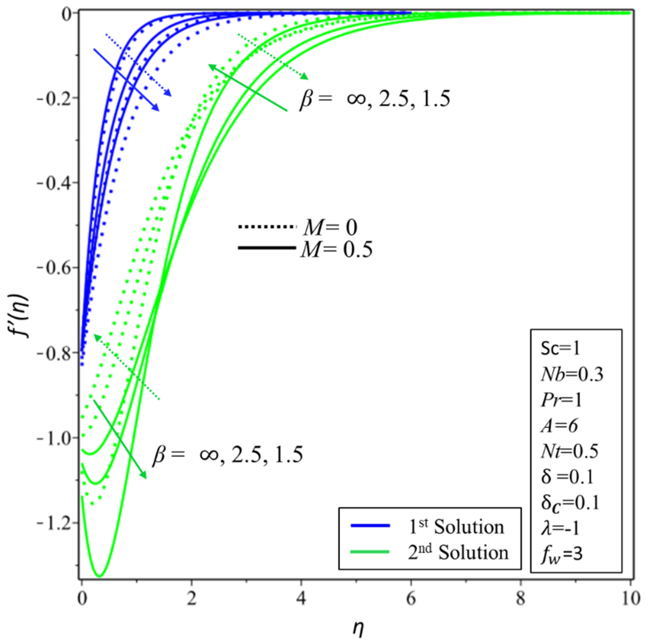
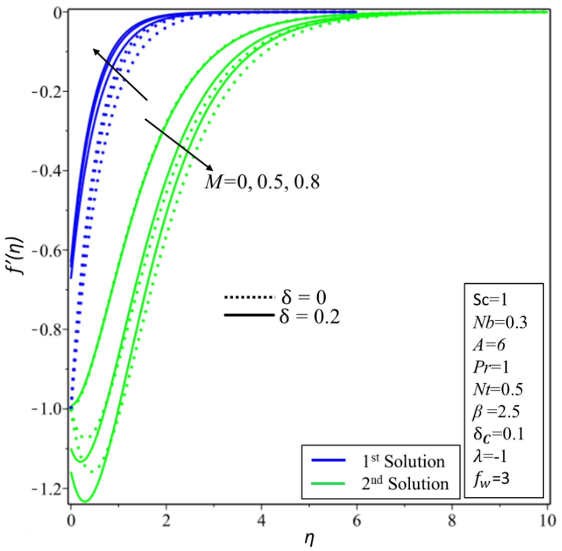
• For the stable solution, the velocity profile decreases for higher values of Casson parameter $\beta$ and the magnetic field $M$;
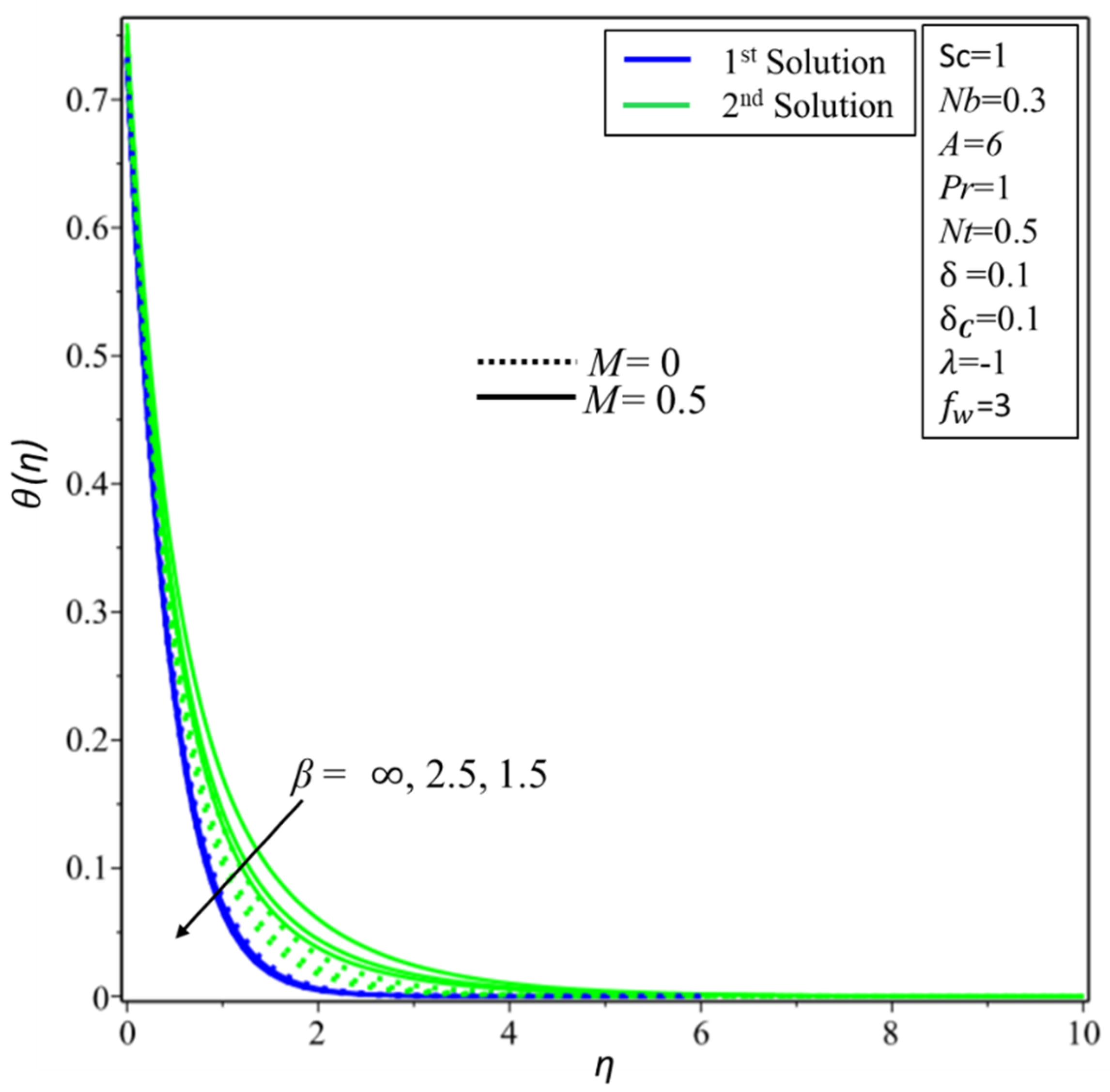
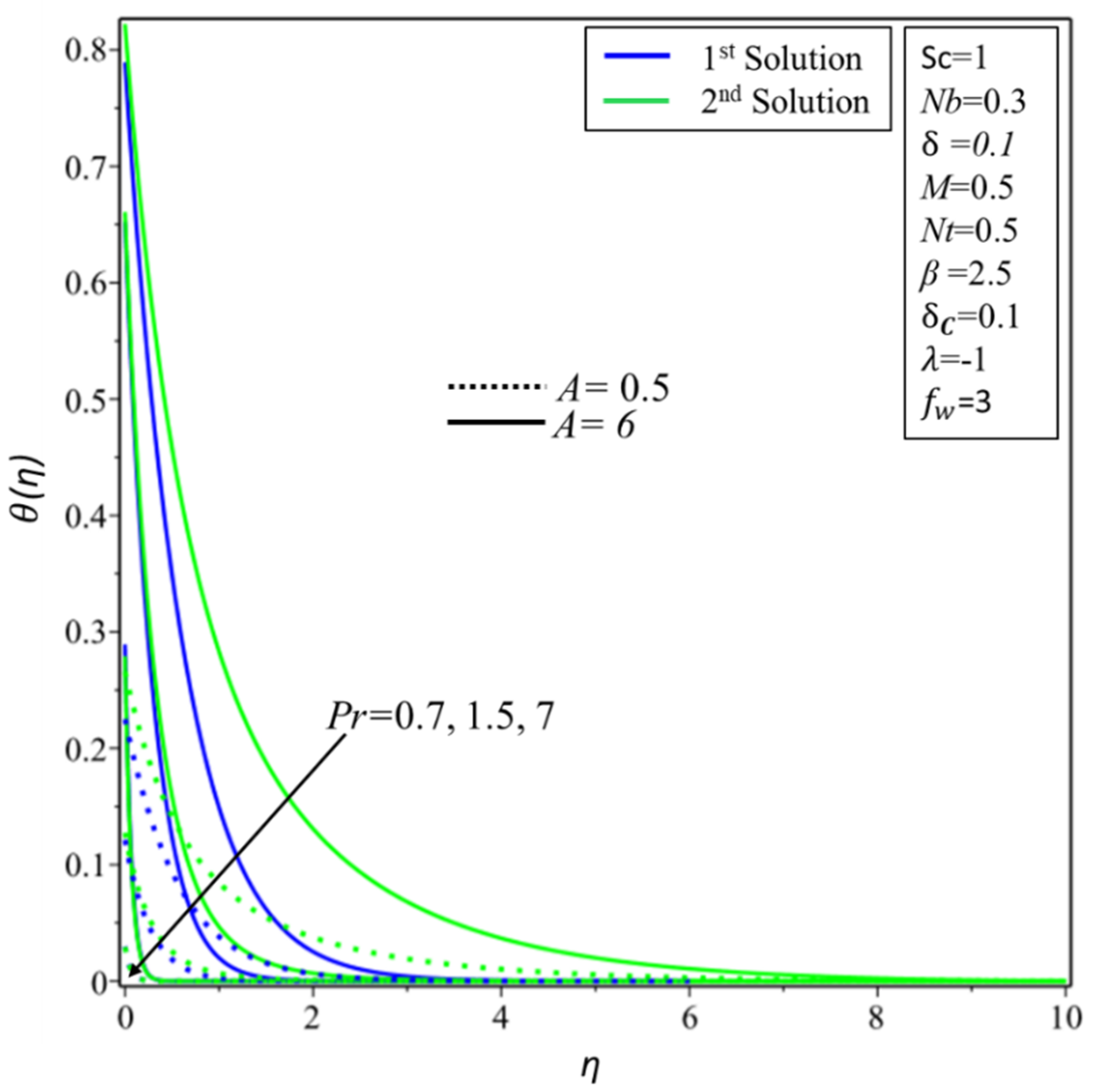
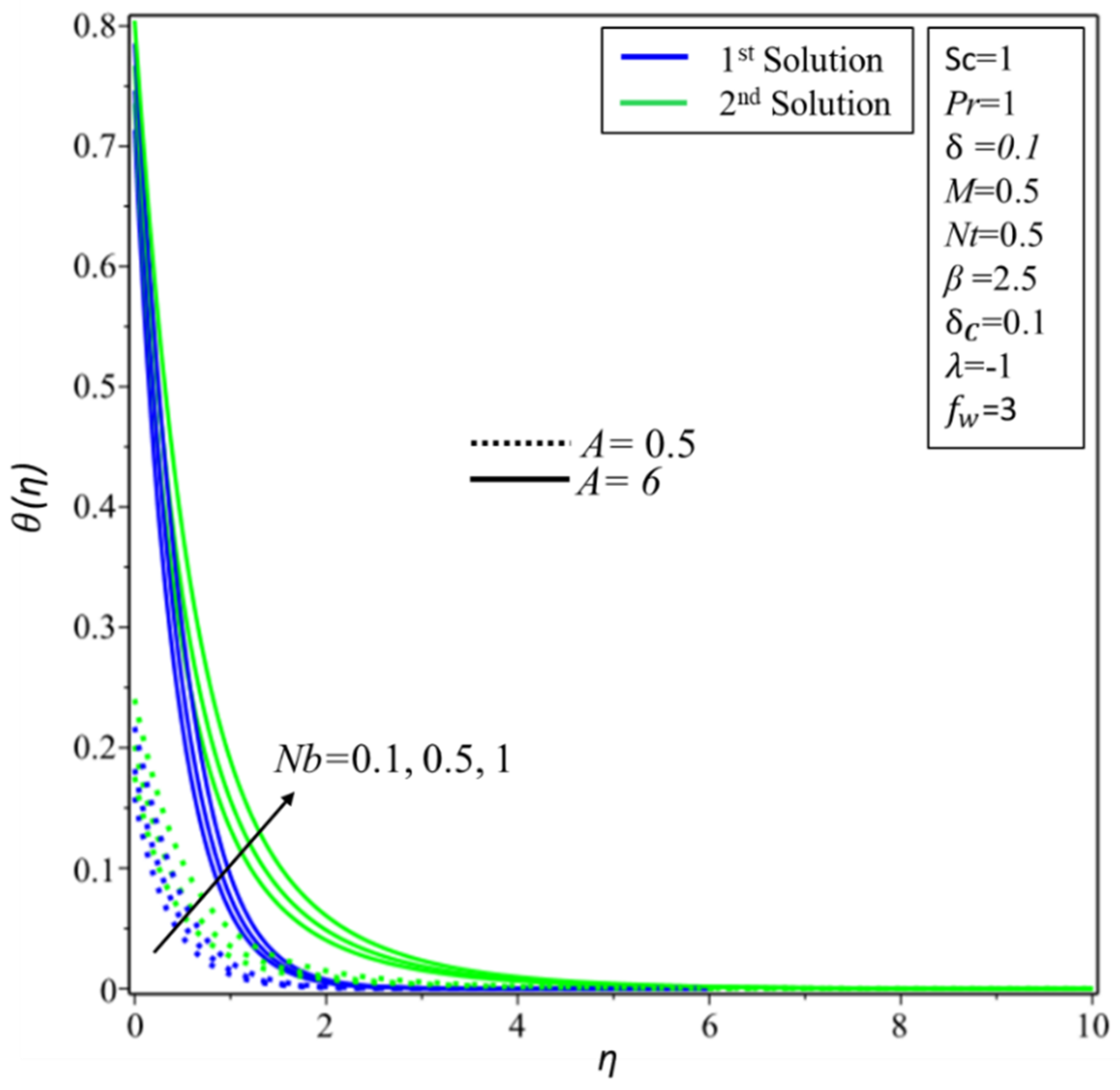
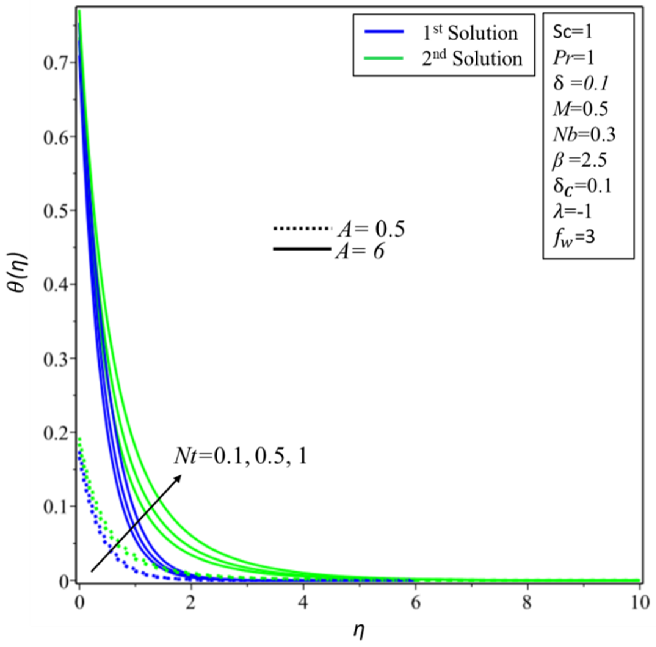
• With a rise in the intensity of the convection parameter $A$, the thermal boundary layer is enhanced. Yet, the Prandtl number $Pr$ has the inverse relationship with the temperature profile in both solutions.
• Stability analysis reveals that an unstable (/stable) solution is a second (/first) solution.
• Dual solutions vary, and no solution depends on the parameters involved.

References

1. Li, Z.; Barnoon, P.; Toghraie, D.; Dehkordi, R.B.; Afrand, M. Mixed convection of non-Newtonian nanofluid in an H-shaped cavity with cooler and heater cylinders filled by a porous material: Two phase approach. Adv. Powder Technol. 2019, 30, 2666–2685. [Google Scholar] [CrossRef]
2. Arabpour, A.; Karimipour, A.; Toghraie, D.; Akbari, O.A. Investigation into the effects of slip boundary condition on nanofluid flow in a double-layer microchannel. J. Therm. Anal. Calorim. 2018, 131, 2975–2991. [Google Scholar] [CrossRef]
3. Barnoon, P.; Toghraie, D. Numerical investigation of laminar flow and heat transfer of non-Newtonian nanofluid within a porous medium. Powder Technol. 2018, 325, 78–91. [Google Scholar] [CrossRef]
4. Yasmeen, S.; Asghar, S.; Anjum, H.J.; Ehsan, T. Analysis of Hartmann boundary layer peristaltic flow of Jeffrey fluid: Quantitative and qualitative approaches. Commun. Nonlinear Sci. Numer. Simul. 2019, 76, 51–65. [Google Scholar] [CrossRef]
5. Lund, L.A.; Omar, Z.; Khan, I. Steady incompressible magnetohydrodynamics Casson boundary layer flow past a permeable vertical and exponentially shrinking sheet: A stability analysis. Heat Transf. Asian Res. 2019, 48, 3538–3556. [Google Scholar] [CrossRef]
6. Lund, L.A.; Omar, Z.; Khan, I. Mathematical analysis of magnetohydrodynamic (MHD) flow of micropolar nanofluid under buoyancy effects past a vertical shrinking surface: Dual solutions. Heliyon 2019, 5, e02432. [Google Scholar] [CrossRef] [Green Version]
7. Dero, S.; Rohni, A.M.; Saaban, A. MHD micropolar nanofluid flow over an exponentially stretching/shrinking surface: Triple solutions. J. Adv. Res. Fluid Mech. Therm. Sci. 2019, 56, 165–174. [Google Scholar]
8. Nakamura, M.; Sawada, T. Numerical study on the flow of a non-Newtonian fluid through an axisymmetric stenosis. J. Biomech. Eng. 1988, 110, 137–143. [Google Scholar] [CrossRef]
9. Mustafa, M.; Hayat, T.; Pop, I.; Aziz, A. Unsteady boundary layer flow of a Casson fluid due to an impulsively started moving flat plate. Heat Transf. Asian Res. 2011, 40, 563–576. [Google Scholar] [CrossRef]
10. Nadeem, S.; Haq, R.U.; Lee, C. MHD flow of a Casson fluid over an exponentially shrinking sheet. Sci. Iran. 2012, 19, 1550–1553. [Google Scholar] [CrossRef] [Green Version]
11. Qayyum, M.; Khan, H.; Khan, O. Slip analysis at fluid-solid interface in MHD squeezing flow of casson fluid through porous medium. Results Phys. 2017, 7, 732–750. [Google Scholar] [CrossRef]
12. Buongiorno, J. Convective transport in nanofluids. J. Heat Transf. 2006, 128, 240–250. [Google Scholar] [CrossRef]
13. Lund, L.A.; Omar, Z.; Dero, S.; Khan, I. Linear stability analysis of MHD flow of micropolar fluid with thermal radiation and convective boundary condition: Exact solution. Heat Transf. Asian Res. 2020, 49, 461–476. [Google Scholar] [CrossRef]
14. Daniali, O.A.; Toghraie, D.; Eftekhari, S.A. Thermo-hydraulic and economic optimization of Iranol refinery oil heat exchanger with Copper oxide nanoparticles using MOMBO. Phys. A:Stat. Mech. Its Appl. 2020, 540, 123010. [Google Scholar] [CrossRef]
15. Hayat, T.; Ullah, I.; Waqas, M.; Alsaedi, A. Attributes of Activation Energy and Exponential Based Heat Source in Flow of Carreau Fluid with Cross-Diffusion Effects. J. Non-Equilib. Thermodyn. 2019, 44, 203–213. [Google Scholar] [CrossRef]
16. Mabood, F.; Das, K. Outlining the impact of melting on MHD Casson fluid flow past a stretching sheet in a porous medium with radiation. Heliyon 2019, 5, e01216. [Google Scholar] [CrossRef] [PubMed] [Green Version]
17. Nagendra, N.; Amanulla, C.H.; Reddy, M.S.; Prasad, V.R. Hydromagnetic Flow of Heat and Mass Transfer in a Nano Williamson Fluid Past a Vertical Plate with Thermal and Momentum Slip Effects: Numerical Study. Nonlinear Eng. 2019, 8, 127–144. [Google Scholar] [CrossRef]
18. Ramesh, K.; Kumar, D.; Devakar, M. Electrokinetically modulated flow of couple stress magneto-nanofluids in a microfluidic channel. Heat Transf. Asian Res. 2019, 48, 379–397. [Google Scholar] [CrossRef] [Green Version]
19. Karbasifar, B.; Akbari, M.; Toghraie, D. Mixed convection of Water-Aluminum oxide nanofluid in an inclined lid-driven cavity containing a hot elliptical centric cylinder. Int. J. Heat Mass Transf. 2018, 116, 1237–1249. [Google Scholar] [CrossRef]
20. William, B.B. Magnetohydrodynamic-hypersonic flow past a blunt body. J. Aerosp. Sci. 1958, 25, 685–690. [Google Scholar]
21. William, B.B. The stagnation-point boundary layer in the presence of an applied magnetic field. J. Aerosp. Sci. 1961, 28, 610–611. [Google Scholar]
22. Eastman, T.E.; Hones, E.W.; Bame, S.J.; Asbridge, J.R. The magnetospheric boundary layer: Site of plasma, momentum and energy transfer from the magnetosheath into the magnetosphere. Geophys. Res. Lett. 1976, 3, 685–688. [Google Scholar] [CrossRef]
23. Hossain, M.A. Viscous and Joule Heating Effects on MHD Free Convection Flow with Variable Plate Temperature (No. IC--90/265); International Centre for Theoretical Physics: Trieste, Italy, 1990. [Google Scholar]
24. Prasad, K.V.; Vaidya, H.; Makinde, O.D.; Setty, B.S. MHD Mixed Convective Flow of Casson Nanofluid over a Slender Rotating Disk with Source/Sink and Partial Slip Effects. Defect Diffus. Forum 2016, 392, 92–122. [Google Scholar] [CrossRef]
25. Toghraie, D.; Abdollah, M.M.D.; Pourfattah, F.; Akbari, O.A.; Ruhani, B. Numerical investigation of flow and heat transfer characteristics in smooth, sinusoidal and zigzag-shaped microchannel with and without nanofluid. J. Therm. Anal. Calorim. 2018, 131, 1757–1766. [Google Scholar] [CrossRef]
26. Mashayekhi, R.; Arasteh, H.; Toghraie, D.; Motaharpour, S.H.; Keshmiri, A.; Afrand, M. Heat transfer enhancement of Water-Al2O3 nanofluid in an oval channel equipped with two rows of twisted conical strip inserts in various directions: A two-phase approach. Comput. Math. Appl. 2019, 79, 2203–2215. [Google Scholar] [CrossRef]
27. Sakiadis, B.C. Boundary-layer behavior on continuous solid surfaces: I. Boundary-layer equations for two-dimensional and axisymmetric flow. Aiche J. 1961, 7, 26–28. [Google Scholar] [CrossRef]
28. Crane, L.J. Flow past a stretching plate. Z. Angew. Math. Phys. 1970, 21, 645–647. [Google Scholar] [CrossRef]
29. Gupta, P.S.; Gupta, A.S. Heat and mass transfer on a stretching sheet with suction or blowing. Can. J. Chem. Eng. 1977, 55, 744–746. [Google Scholar] [CrossRef]
30. Grubka, L.J.; Bobba, K.M. Heat transfer characteristics of a continuous stretching surface with variable temperature. ASME J. Heat Transf. 1985, 107, 248–250. [Google Scholar] [CrossRef]
31. Andersson, H.I.; Aarseth, J.B.; Dandapat, B.S. Heat transfer in a liquid film on an unsteady stretching surface. Int. J. Heat Mass Transf. 2000, 43, 69–74. [Google Scholar] [CrossRef]
32. Khan, W.A.; Pop, I. Boundary-layer flow of a nanofluid past a stretching sheet. Int. J. Heat Mass Transf. 2010, 53, 2477–2483. [Google Scholar] [CrossRef]
33. Weidman, P.D.; Kubitschek, D.G.; Davis, A.M.J. The effect of transpiration on self-similar boundary layer flow over moving surfaces. Int. J. Eng. Sci. 2006, 44, 730–737. [Google Scholar] [CrossRef]
34. Harris, S.D.; Ingham, D.B.; Pop, I. Mixed convection boundary-layer flow near the stagnation point on a vertical surface in a porous medium: Brinkman model with slip. Transport. Porous Media 2009, 77, 267–285. [Google Scholar] [CrossRef]
35. Merkin, J.H. On dual solutions occurring in mixed convection in a porous medium. J. Eng. Math. 1986, 20, 171–179. [Google Scholar] [CrossRef]
36. Roşca, A.V.; Pop, I. Flow and heat transfer over a vertical permeable stretching/shrinking sheet with a second order slip. Int. J. Heat Mass Transf. 2013, 60, 355–364. [Google Scholar] [CrossRef]
37. Rahman, M.M.; Rosca, A.V.; Pop, I. Boundary layer flow of a nanofluid past a permeable exponentially shrinking surface with convective boundary condition using Buongiorno’s model. Int. J. Numer. Methods Heat Fluid Flow 2015, 25, 299–319. [Google Scholar] [CrossRef]
38. Mustafaa, M.; Hayat, T.; Obaidat, S. Boundary layer flow of a nanofluid over an exponentially stretching sheet with convective boundary conditions. Int. J. Numer. Methods Heat Fluid Flow 2013, 23, 945–959. [Google Scholar] [CrossRef]
39. Miklavčič, M.; Wang, C. Viscous flow due to a shrinking sheet. Q. Appl. Math. 2006, 64, 283–290. [Google Scholar] [CrossRef] [Green Version]
40. Fang, T.; Zhang, J. Closed-form exact solutions of MHD viscous flow over a shrinking sheet. Commun. Nonlinear Sci. Numer. Simul. 2009, 14, 2853–2857. [Google Scholar] [CrossRef]
41. Bhattacharyya, K. Boundary layer flow and heat transfer over an exponentially shrinking sheet. Chin. Phys. Lett. 2011, 28, 074701. [Google Scholar] [CrossRef]
Figure 1. Procedure of three-stage Lobatto IIIa formula along with stability analysis.
Symmetry 12 01162 g001
Figure 2. Effect of λ on f′(η).
Symmetry 12 01162 g002
Figure 3. f ( 0 ) for different values of λ.
Symmetry 12 01162 g003
Figure 4. θ ( 0 ) for different values of λ .
Symmetry 12 01162 g004
Figure 5. ( 0 ) for different values of λ .
Symmetry 12 01162 g005
Figure 6. f ( 0 ) for different values of f w by varying β .
Symmetry 12 01162 g006
Figure 7. θ ( 0 ) for different values of f w by varying β .
Symmetry 12 01162 g007
Figure 8. ( 0 ) for different values of f w by varying β .
Symmetry 12 01162 g008
Figure 9. f ( η ) for different values of β by varying M .
Symmetry 12 01162 g009
Figure 10. f ( η ) for different values of M by varying δ.
Symmetry 12 01162 g010
Figure 11. θ ( η ) for different values of β by varying M .
Symmetry 12 01162 g011
Figure 12. θ ( η ) for different values of P r by varying A .
Symmetry 12 01162 g012
Figure 13. θ ( η ) for different values of N b by varying A .
Symmetry 12 01162 g013
Figure 14. θ ( η ) for different values of N t by varying A .
Symmetry 12 01162 g014
Figure 15. ( η ) for different values of N b by varying δ c .
Symmetry 12 01162 g015
Figure 16. ( η ) for different values of N t by varying δ c .
Symmetry 12 01162 g016
Figure 17. ( η ) for different values of S c by varying δ c .
Symmetry 12 01162 g017