Investigating Long-Range Dependence of Emerging Asian Stock Markets Using Multifractal Detrended Fluctuation Analysis

Abstract

The use of multifractal approaches has been growing because of the capacity of these tools to analyze complex properties and possible nonlinear structures such as those in financial time series. This paper analyzes the presence of long-range dependence and multifractal parameters in the stock indices of nine MSCI emerging Asian economies. Multifractal Detrended Fluctuation Analysis (MFDFA) is used, with prior application of the Seasonal and Trend Decomposition using the Loess (STL) method for more reliable results, as STL separates different components of the time series and removes seasonal oscillations. We find a varying degree of multifractality in all the markets considered, implying that they exhibit long-range correlations, which could be related to verification of the fractal market hypothesis. The evidence of multifractality reveals symmetry in the variation trends of the multifractal spectrum parameters of financial time series, which could be useful to develop portfolio management. Based on the degree of multifractality, the Chinese and South Korean markets exhibit the least long-range dependence, followed by Pakistan, Indonesia, and Thailand. On the contrary, the Indian and Malaysian stock markets are found to have the highest level of dependence. This evidence could be related to possible market inefficiencies, implying the possibility of institutional investors using active trading strategies in order to make their portfolios more profitable.

1. Introduction

A financial system is an integral part of an economy, allowing for the exchange of funds between lenders, borrowers, investors, and government entities, and efficient resource allocation. Correct understanding of financial markets’ structures is important for the design of appropriate public policies, investment strategies and portfolios, or taxation and legal frameworks, which are major ingredients of a well-structured economy. The study of financial markets has long been based on the Random Walk Hypothesis (RWH) introduced by the authors of [1], which assumes that stock prices are described by a random walk, this being the basis of a fundamental theory of financial markets, namely, the Efficient Market Hypothesis (EMH) proposed in [2]. In its weak form, the efficiency hypothesis presumes that markets are inherently efficient to readily adjust their assets’ prices to any new information, preventing investors from having abnormal returns. However, market structures do not behave in this way and different research reveals that stock markets have ubiquitous properties [3,4,5], with issues described in the literature as stylized facts like fat tails [6], long-term correlations [7], volatility clustering [8], fractals/multifractals [9], and chaos [10], with these properties making financial markets inconsistent with both EMH and RWH [11]. These inconsistencies required more logical explanation of market movements than the ones described by the EMH. Some questions were answered by proving that fractal models, incorporating issues like geometric shape, parts of which can be isolated, reflect more realistic market activity. Based on this, the authors of [12,13] developed the Fractal Market Hypothesis (FMH). This is less restrictive as it considers, for example, the possibility of investors’ heterogeneous behavior, which according to theory is the guarantee of market stability [12,13,14].

Although building the FMH dates from the 1990s, the work of Mandelbrot [3,4,5] is seminal, with the introduction of fractal geometry to investigate the behavior of cotton prices and finding that commodity prices do not exhibit a random walk behavior. Fractal geometry was inspirational for the study of financial markets, as, in general, time series of financial assets’ prices show similar complex multifractal patterns to those found in some commodities. Based on the fractal theory, some initial studies used Detrended Fluctuation Analysis (DFA) as a monofractal approach to investigate stock markets’ long-range dependence [12,14,15]. With an R/S analysis, the authors of [16,17] identified the existence of monofractality. However, this is a property which could not describe correctly the behavior of correlation functions [18]. Later, research in this particular area showed that a single scaling component used in a monofractal analysis to study prices’ complex multifractal structures is not sufficient, opening the way for the development of more robust techniques like Multifractal Detrended Fluctuation Analysis (MFDFA) [7,19] and the partition function method [20,21,22]. By using the fractal dimension algorithm, the authors of [23] analyzed the performance of the Fama and French [24] five-factor model including the Hurst exponent as an additional factor. The authors reported that the significance of the H factor is greater than the momentum factor and similar to others such as the capitalization and book-to-market factors.

Multifractality is central in the study of complexity and has applications in almost all essential areas of scientific research from physics to economics, but also in other natural and social sciences such as chemistry, hydrology, or psychology, or even other research areas like linguistics, the environment or even music (see, e.g., in [25,26,27,28,29,30,31,32] among others). In particular, MFDFA is a strong tool, capable of detecting long-term dependence even in the presence of non-stationarity [33]. In the context of financial markets, it could help to determine the existence of long-range dependencies linking them to the EMH and reveal the extent of inefficiency [34]. This method has already been applied in several fields, including finance [5,20,35,36,37], revealing the existence of multifractality in financial markets [38,39,40,41,42].

We find a wide gap in the literature regarding in-depth analysis of the fractal behavior of emerging markets in general and Asian markets in particular. In order to fill this gap, this paper is unique and extends the existing literature in three ways. First, this study provides evidence of long-range dependence in nine Morgan Stanley Capital International (MSCI) emerging Asian markets, namely, China, South Korea, India, Pakistan, Malaysia, Indonesia, the Philippines, Thailand, and Taiwan. Using daily price data up to 02 April 2020, this study examines the behavior of nine stock markets over the long run. Second, the use of Seasonal and Trend Decomposition using Loess (STL) before applying MFDFA, in order to decompose the original time series of stock returns, isolating its values from possible seasonal oscillations [11]. This is an advantage because STL can handle several different types of seasonality, is robust to the existence of outliers, and can detect seasonal variations over time. According to the work in [43], the application of STL can identify the dynamics of stock returns at the same time as assuring reliability by decomposing the time series after removing seasonal components. Third, the use of a robust Econophysics methodology such as MFDFA, as a generalization of the original DFA proposed in [19], will allow us to detect the pattern of multifractal behavior in emerging Asian stock markets. The main results of this paper show that the Chinese and South Korean stock markets have the lowest levels of multifractality, while the Indian and Malaysian ones show the highest levels. Moreover, only the Chinese and Indonesian stock markets indicate persistent fluctuation, while the remaining seven stock markets show anti-persistent patterns. Overall, the stock markets considered show long-range dependence.

The remainder of the paper is structured as follows. Section 2 presents the data and describes the methodology employed, Section 3 shows the empirical results, and Section 4 concludes.

2. Literature Review

In order to analyze the existence of dependence in financial markets, over time researchers have used both traditional econometric techniques and fractal models. Despite a large number of variations in methodologies, most studies suggest that financial markets show the existence of dependence, regardless of the type of sample under analysis. Most research is mainly focused on developed countries’ levels of dependence, with several studies finding ample empirical evidence of that pattern in European stock markets [44,45], while the absence of dependence is rare in the literature [46,47,48].

The empirical tests used in these studies include methodologies like parametric autocorrelation, unit root and variance ratio tests, nonparametric tools, filter rules, or application of GARCH (Generalized Autoregressive Conditional Heteroskedasticity) models. Developments in the market microstructure modeling suggest that time is an important source of information and should be modeled as well. To incorporate this important consideration, the authors of [49] developed the Autoregressive Conditional Duration (ACD) model, which explicitly focuses on the modeling of times between events and relies on linear parameterization. As demonstrated in [49,50], the GARCH and ACD models share many common features. For instance, the authors of [51] developed an application of ACD-GARCH models with the purpose of forecasting future volatilities and confirmed that the realized volatility developed in [52] seems to outperform any of the GARCH models for ultra-high frequent data. According to the work in [49], nonlinearity models suggest that the standard ACD model fails to capture nonlinear dependence.

Several studies analyze financial markets applying different versions of these models. For instance, the authors of [47] used a rolling window variance ratio to estimate the weak form of efficiency and found a varying degree of market predictability, in the case of European stock markets. By using the autocorrelation analysis, runs test, variance ratio test, and a GARCH-in-mean model, the work in [53] confirms the existence of dependence in seven European stock markets. For a comparative analysis, the authors of [54] applied linear and nonlinear unit root tests to investigate the efficiency of emerging economies and found distinct results when comparing linear and nonlinear unit root tests: nonlinear ones suggested that dependence could exist, while linear tests suggested the opposite. Similar findings are reported in [42] using unit root tests, nonparametric runs test, and joint variance tests.

Empirical study of less developed and developing financial markets offers more research opportunities as they are generally considered as having higher dependence levels in an overall integrated global financial system, related to those markets’ levels of immaturity. More data available makes it possible to analyze these markets. Various studies reveal that stock markets in the Middle East and North Africa (MENA) and Asia could suffer from inefficiency [55,56]. For instance, the authors of [55] documented the presence of the adaptive market hypothesis (AMH) by using the daily data of the TEPIX index in the Tehran Stock Exchange (TSE), in Iran. Using more conventional econometric models, such as GARCH, autocorrelation, and runs tests, and considering eight Asian emerging market indices, the work in [56] provides evidence of a varying degree of dependence. From a different perspective, the authors of [57] evaluate the relationship between market development and multifractality degree in developed and emerging stock markets, finding that emerging stock markets have a higher degree of multifractality than developed ones. Focusing particularly on the Russian stock market, the authors of [58] classified the Russian Stock market as one of the emerging countries and argue that the multifractal structures of Russian stock markets are destroyed by the Russian 1998 and global financial crises. In a study of frontier markets, the authors of [59] test the weak form of efficiency by using mutual information and DFA, and show that frontier stock markets in Europe and America have less evidence of dependence than those in the Middle East. Recently, the authors of [11] used MFDFA to compare multifractal properties in several Central and Eastern European (CEE) markets finding evidence of long-term dependence, concluding on the inefficiency of the markets studied, probably due to them not yet having the necessary degree of maturity. Combining MFDFA and copula models, the authors of [60] used a bootstrap experiment to analyze how the 2008 and 2010 crises impacted on European stock markets, finding evidence of long memory in the first crisis, but not in the second. Furthermore, the findings of copula models reveal the existence of financial contagion. Moreover, using the global financial crisis as a benchmark, the authors of [33] also employed MFDFA and found that Islamic stock markets still had evidence of dependence in the crisis period, when compared with other developed markets.

In summary, we can conclude that stock market efficiency is estimated by both conventional econometric and econophysics models. However, conventional models fail to explain fat tails, long-term correlation, volatility clustering, and multifractality in financial markets. Recent developments on information efficiency in emerging markets can be found in [61], while prior literature on efficiency of emerging markets can be found in [44,62].

3. Materials and Methods

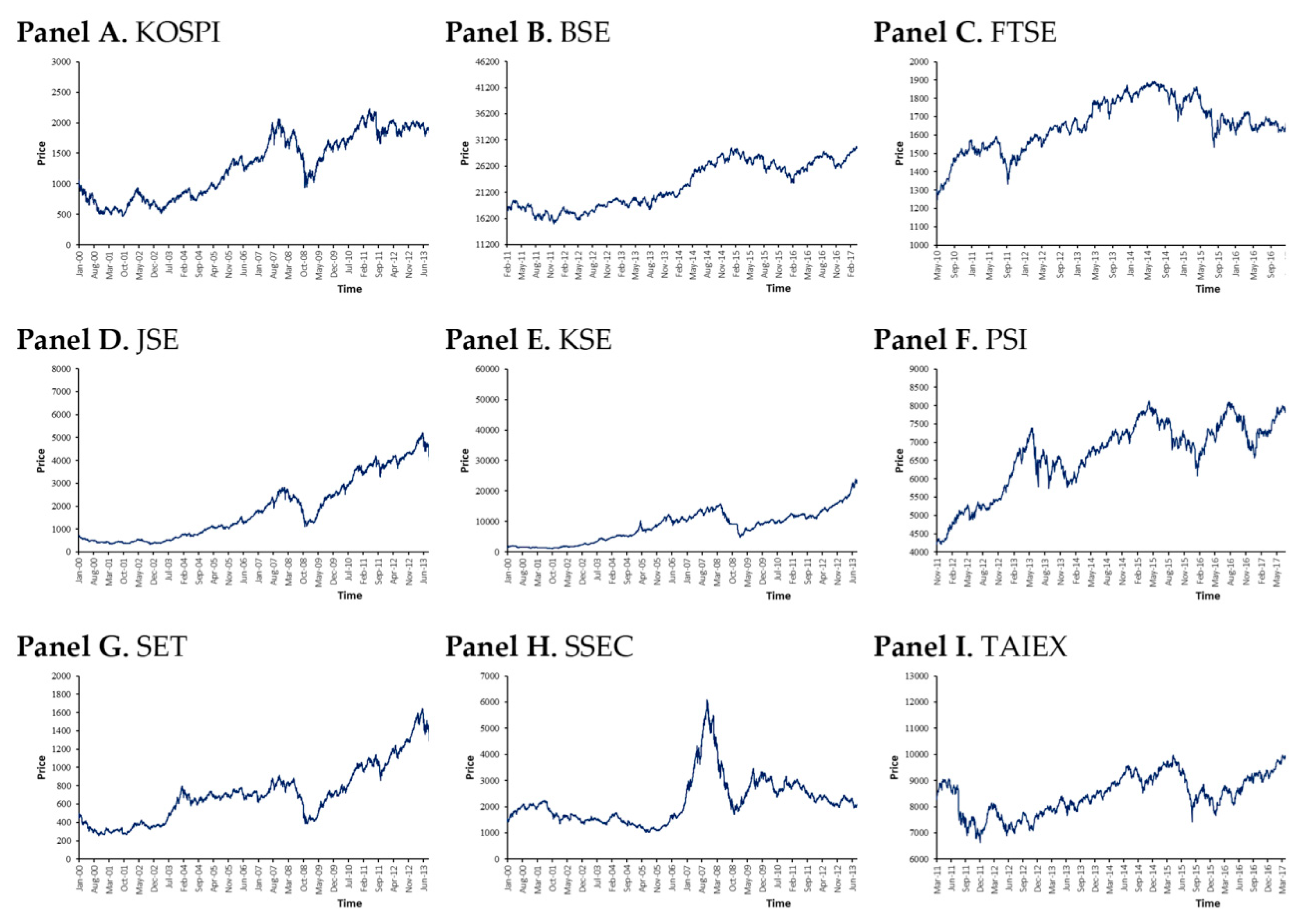
3.1. Data Description

For this study, we retrieved data of daily closing indices for nine emerging Asian stock markets from DataStream, up to 02 April 2020. Morgan Stanley Capital International (MSCI) classifies stock markets as developed, emerging, or frontier, based on several criteria including size, accessibility, liquidity, and development (for more details about classification criteria and membership, see MSCI website). Asian markets are heavily weighted on the emerging market index, namely, the stock markets of China (33%), South Korea (13.02%), Taiwan (11.35%), and India (9.16%). MSCI updates their classifications and the number of countries in each category varies from time to time.

Table 1. Description of the stock indices used.

S.No.	Country	Index Symbol	Data Range	Observation (Daily)
1	India	BSE	24-Feb-2011 to 1-Apr-2020	2252
2	Malaysia	FTSE	20-May-2010 to 2-Apr-2020	2441
3	Indonesia	JSE	4-Jan-2000 to 2-Apr-2020	4941
4	South Korea	KOSPI	4-Jan-2000 to 1-Apr-2020	5000
5	Pakistan	KSE	3-Jan-2000 to 31-Mar-2020	5000
6	Philippines	PSE	2-Nov-2011 to 1-Apr-2020	2049
7	Thailand	SET	4-Jan-2000 to 2-Apr-2020	4958
8	China	SSEC	4-Jan-2000 to 2-Apr-2020	4908
9	Taiwan	TAIEX	17-Mar-2011 to 1-Apr-2020	2233

provides the information about the data used in this paper, namely, the country, the stock market, and information about the sample and the number of observations (samples vary according to data availability).

In Appendix A, Figure A1 illustrates the daily movements of the stock market indexes up to 02-Apr-2020. Daily returns are calculated with the usual logarithm difference, i.e.,

$$r\left(t\right)=\ln p\left(t\right)-\ln p\left(t-1\right),$$

(1)

with $p\left(t\right)$ being the closing price of a given index at time t.

3.2. Methodology

Our main objective of measuring the multifractality pattern of emerging Asian markets is fulfilled using multifractal detrended fluctuation analysis (MFDFA). Previously, STL is applied in order to decompose return series according to the authors of [63]. In order to check robustness, we also developed the Brock–Dechert–Scheinkman (BDS) test. As this is a common test, and also due to space constraints, we do not describe this test, with the details being found in [64,65,66].

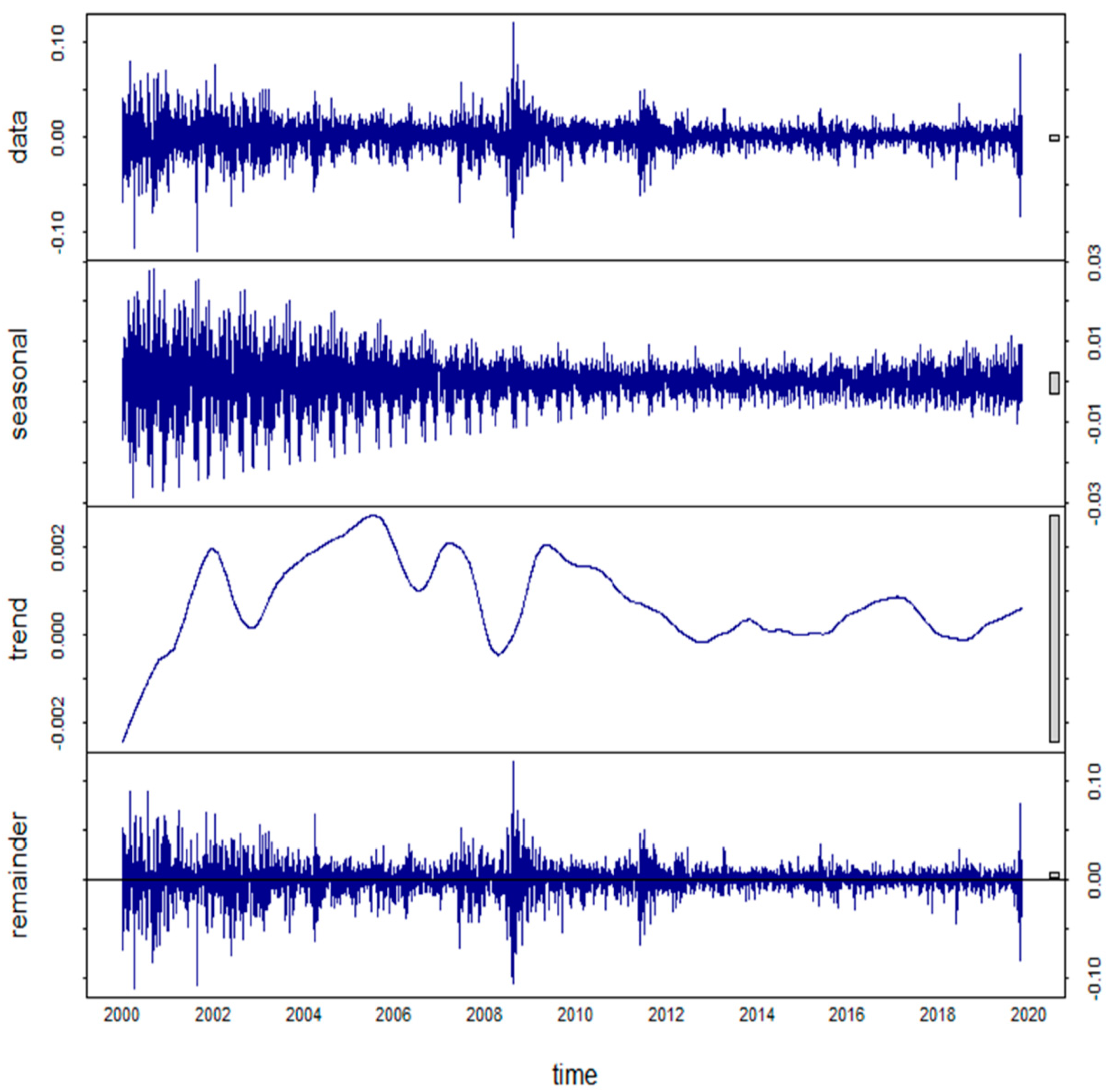
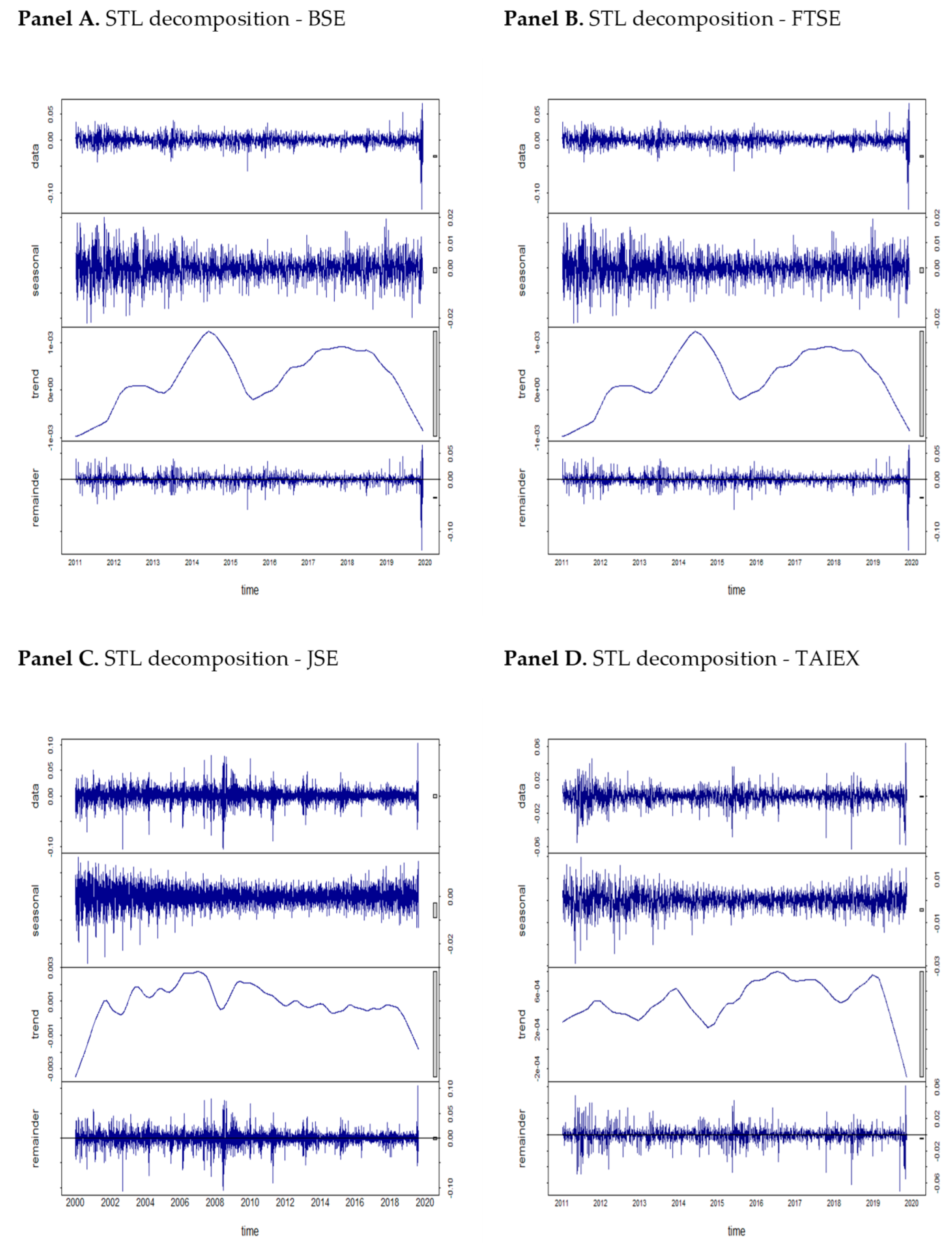
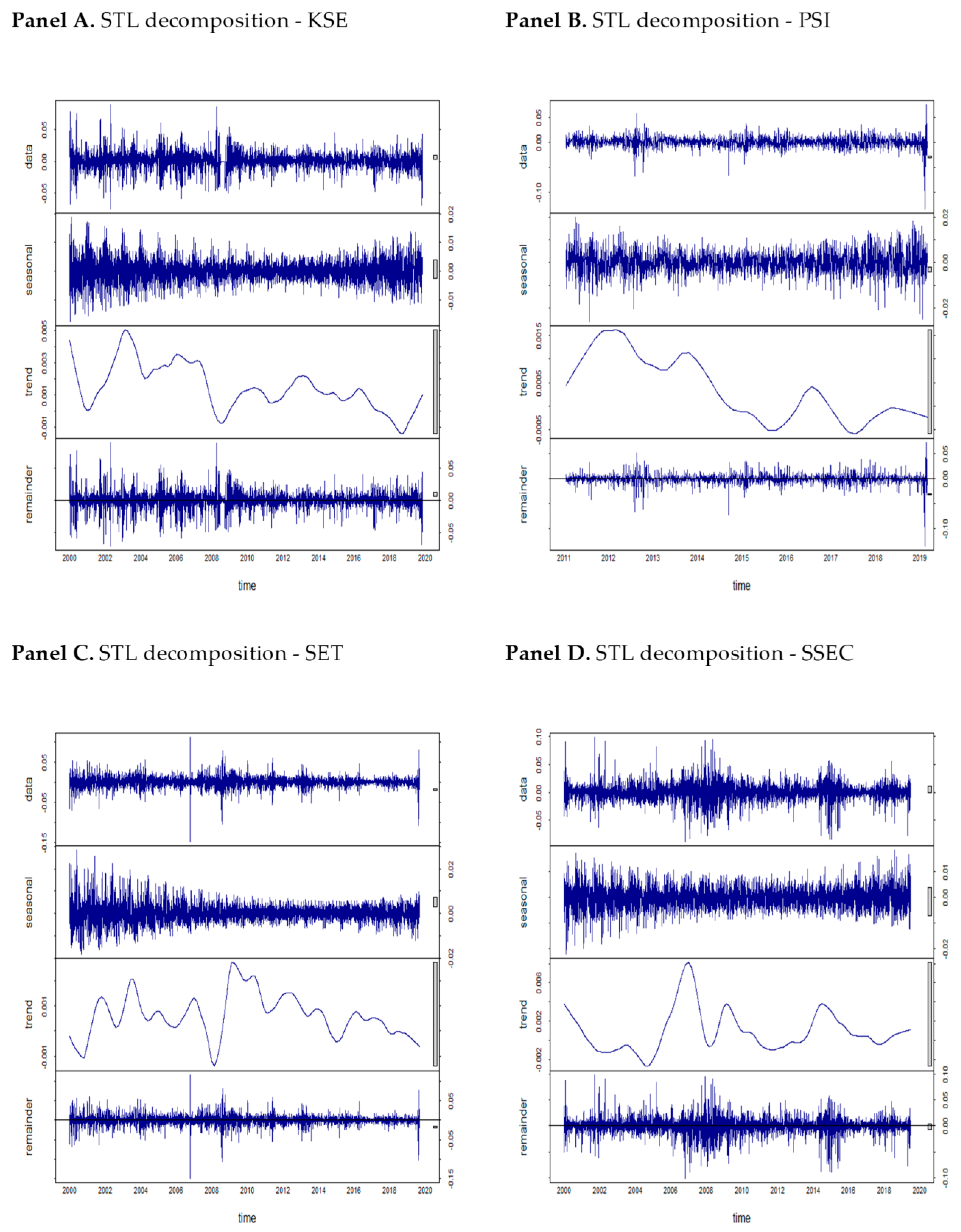
3.2.1. Seasonal and Trend Decomposition Using Loess (STL)

The main purpose of this study is to capture the inner dynamics of the stock returns in emerging Asian markets. In order to reveal these dynamics, we isolate the remainder component by excluding the intrinsically ambiguous seasonal and trend components that could be generated by trading cycles [43]. The use of STL is a flexible and robust technique for decomposing the time series and is a filtering procedure with several advantages over other classical methods (e.g., SEATS or X11). For instance, it allows the seasonal component to change over time, can deal with all types of seasonality (i.e., daily, monthly, quarterly etc.), is more robust to outliers, is flexible in specifying the rate of change of parameters, and is able to deal with missing values. We have applied the STL decomposition method to remove the seasonal components for more reliable results, as proposed, for example, in [11]. STL consists of the decomposition of a given time series, in our case, daily returns, in three different components: a deterministic trend (T), a seasonal component (S), and a stochastic (remainder) component (R) [11,67], i.e.,

$$r\left(t\right)=T\left(t\right)+S\left(t\right)+R\left(t\right).$$

(2)

The separation proposed in Equation (2) is done through a sequence of smoothing operations by using two loops. In the first one, robustness weights are assigned to each data point reflecting how extreme the remainder component $R$ is. In the case of a very large $\left|R\right|$, a small or zero weight is assigned to that data point, reducing or eliminating outliers’ effects. The second loop consists of interactive updates of trend and seasonal components by subtracting the current estimate of the trend from the raw series [64]. After that, data is split into cycle-subseries, in our case, a total of 252 cycle subseries (as this is the average number of trading days per year). Each cycle subseries is locally regressed (thus the name loess) and smoothed being passed in a low-pass filter. S results in the smoothed subseries subtracting the low-pass filter. The trend is obtained calculating the raw data minus S, the final results being the R component which will the input of the final loop.

The R package of “stats” was used [11,43,68], and as we are using daily frequency, we chose for seasonal extraction the number of monthly trading prices (21 days). As previously mentioned, STL deals with any type of seasonality (even time-varying ones), captures the dynamics of asset returns, and is robust to the existence of outliers [43].

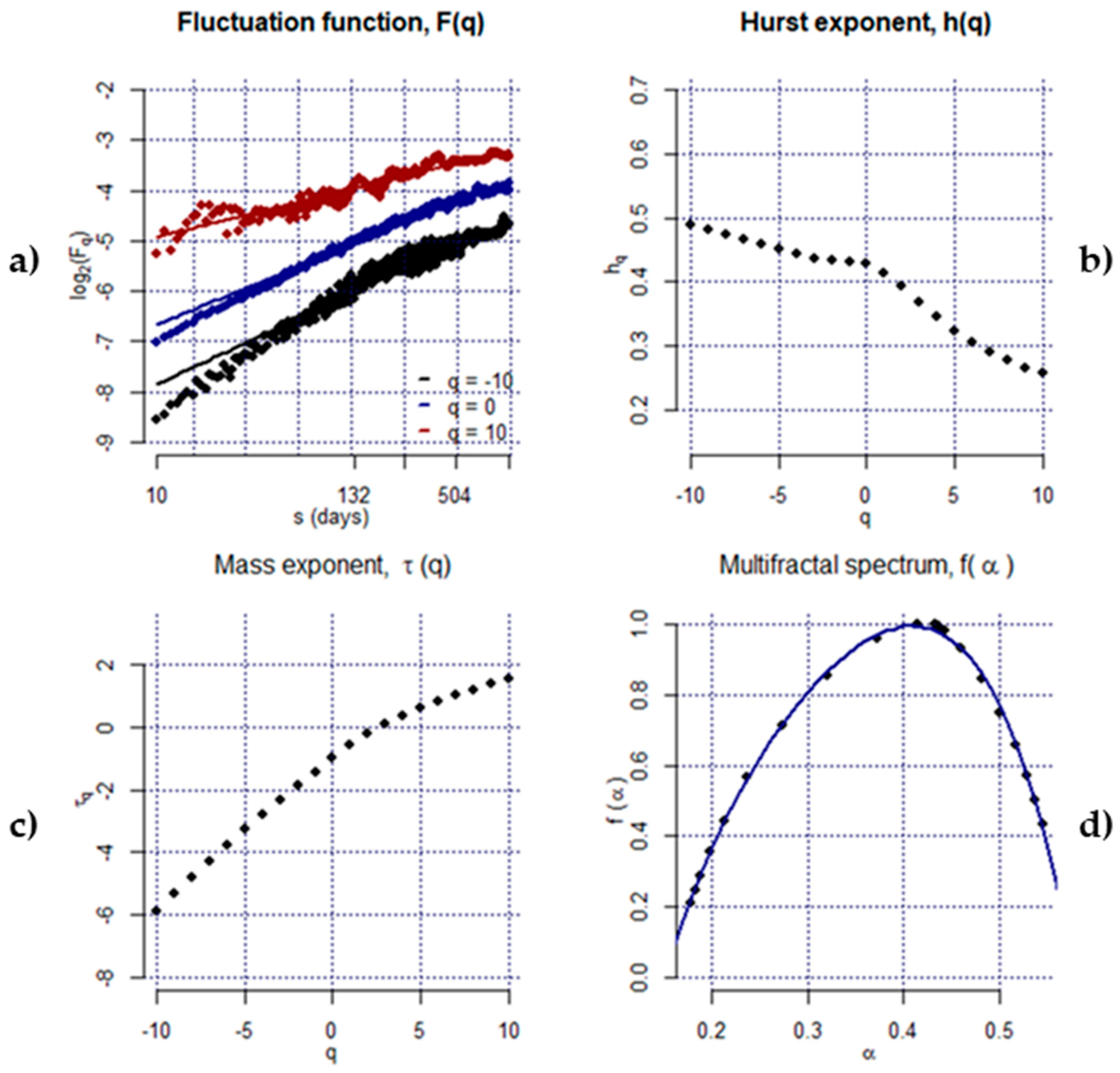
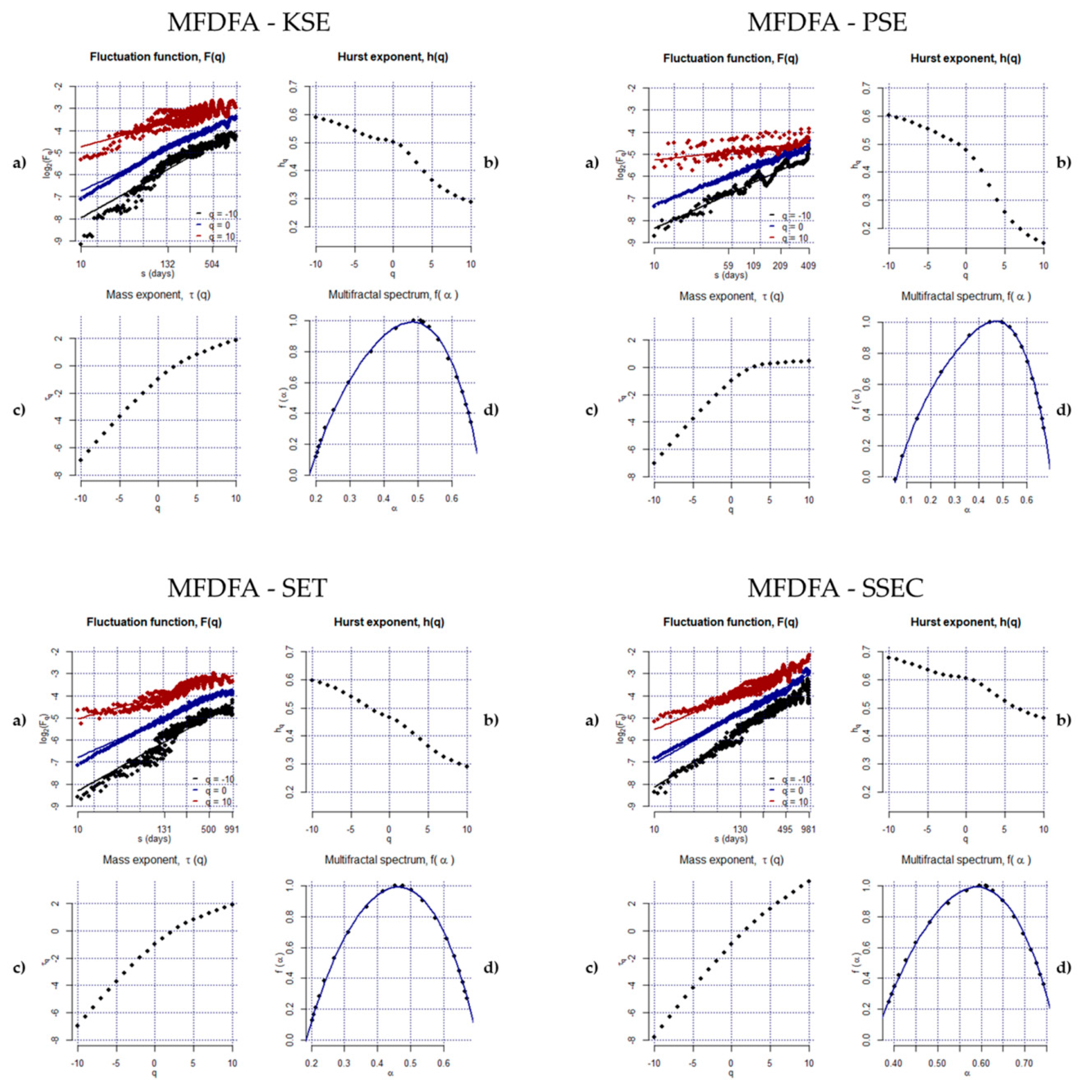
3.2.2. Multifractal Detrended Fluctuation Analysis (MFDFA)

Based on the decomposed STL time series of the remainder component, MFDFA is computed to identify the multifractality pattern of the financial assets’ returns, using the MFDFA package developed by the authors of [43,67] with the [32,69,70] as a possible basis. MFDFA is performed as follows. Considering a time series $\left\{Z_{t, t=1,\dots \dots , N}\right\}$ with length N, the first step considers construction of the profile $X_{\left(k\right)}$, i.e.,

$$X_{\left(k\right)}={{\displaystyle \sum }}_{t=1}^k\left(z_t-\overline{z}\right),$$

(3)

with $k=1,2,3\dots \dots , N$ and $\overline{z}$ the observed mean of the returns. Then, the profile obtained is divided in $N_s$= int $\raisebox{1ex}{$N$}\!\left/ \!\raisebox{-1ex}{$s$}\right.$ nonoverlapping boxes with length s. According to the authors of [19], for the possibility of N being a non-multiple of s, and not to disregard the end of the profile $X_{\left(k\right)}$, the procedure is repeated but starting from the end of the sample, which makes a total of $2N_s$ segments, and following the $10<s<\raisebox{1ex}{$Ns$}\!\left/ \!\raisebox{-1ex}{$5$}\right.$ rule proposed in [15].

The next step is estimation of the local trend, for all $2N_s$ segments, with ordinary least squares, in order to determine the variable given by

$$F^2\left(s,m\right)=\frac{1}{s}{\displaystyle \sum }_{j=1}^s{\left\{X\left[\left(m-1\right)s+j\right]-x_m\left(j\right)\right\}}^2$$

(4)

for the segments between m = 1 and m = N_s, while for the segments between $m=N_{s+1}$ and $m=2N_s$, this is given by

$$F^2\left(s,m\right)=\frac{1}{s}{\displaystyle \sum }_{j=1}^s{\left\{X\left[N-\left(m-N_s\right)s+j\right]-x_m\left(j\right)\right\}}^2$$

(5)

In Equations (4) and (5), $x_{m\left(j\right)}$ represents the polynomial fit of the segments. After averaging, we will obtain the qth-order fluctuation function for any $q\ne 0$ given by

$$F_{q\left(s\right)}={\left\{\frac{1}{2N_s}{\displaystyle \sum }_{\rho =1}^{2N_s}{\left[F^2\left(s,\rho \right)\right]}^{q/2}\right\}}^{1/q}$$

(6)

while for $q=0$ it is equal to

$$F_{0\left(s\right)}=exp\left\{\frac{1}{4N_s}{\displaystyle \sum }_{\rho =1}^{2N_s}ln\left[F^2\left(s,\rho \right)\right]\right\}$$

(7)

If q is negative it represents small fluctuations, while positive values mean larger fluctuations and the specific value of q = 2 represents the DFA exponent.

The value of $F_{q\left(s\right)}$ increases with s, and the performance of a log-log regression between these two variables allows us to obtain the scaling exponent from Equations (6) and (7), which follows the power-law

$$F_{q\left(s\right)}~S^{h\left(q\right)}$$

(8)

The h(q) value is the Hurst exponent, often used to measure the dependence levels of financial assets (see, for example, in [38,39,40]). If h(q) = 0.5, the variable behaves like a random walk, while h(q) > 0.5 and h(q) < 0.5 represent, respectively, persistent and anti-persistent patterns. The value of h(q) could be transformed in a function of Renyi exponent τ(q) given by

$$\tau \left(q\right)=qh\left(q\right)-1$$

(9)

used to measure the mono or multifractality of a given series according to

$$f\left(\mathsf{\alpha }\right)=q\mathsf{\alpha }-\tau \left(q\right)$$

(10)

with α being the Holder exponent given by

$$\mathsf{\alpha }=h_{q }+q\frac{\gamma h_q}{{\gamma }_q}-{\tau }_q$$

(11)

It is possible to identify richer multifractality patterns when h(q) is highly variable.

Based on the width of the exponents given by

$$\Delta h=h_{\left(qmin\right)}-h_{\left(qmax\right)}$$

(12)

it is possible to identify the strength of the multifractality, with h(q) decreasing with the increase of q [57]. Higher values of ∆h imply higher levels of multifractality in the time series.

4. Empirical Results

For illustration purposes, Figure 1 presents the four graphs of the STL decomposition for the Korean stock index (KOSPI) returns with the original daily returns in the 1st row and seasonal, trend, and remainder components in the following rows (in this order). The presence of a seasonal pattern in the Korean stock market can be noticed and agrees with earlier findings [11,71]. However, the trend component shows very small fluctuations around zero. Finally, the remainder component does not follow any regular pattern, experiencing high frequency fluctuations which could be explained by macroeconomic determinants, for example, the 2008–2009 financial crisis [60,72]. Similar findings from STL decomposition are seen for the other eight emerging Asian stock markets, as reported in Figure A2 and Figure A3 in Appendix A.

Application of the BDS test, which checks for the independence of individual time series, allows us to reject always the null hypothesis of independence. This means that we are in the presence of dependent time series which could be compared with the possible multifractal results. All the results can be consulted in Appendix B (

Table A1. BDS test. k represents the dimensions of the test. ^** Denote significance at 1% level.

k	KOSPI	BSE	FTSE	JSE	KSE	PSI	SET	SSEC	TAIEX
2	0.0218 **	0.0090 **	0.0231 **	0.0224 **	0.0351 **	0.0163 **	0.0217 **	0.0166 **	0.0112 **
3	0.0507 **	0.0210 **	0.0444 **	0.0445 **	0.0660 **	0.0307 **	0.0474 **	0.0375 **	0.0250 **
4	0.0735 **	0.0296 **	0.0569 **	0.0595 **	0.0869 **	0.0411 **	0.0661 **	0.0535 **	0.0355 **
5	0.0898 **	0.0354 **	0.0626 **	0.0684 **	0.0982 **	0.0452 **	0.0777 **	0.0630 **	0.0419 **
6	0.0992 **	0.0362 **	0.0636 **	0.0708 **	0.1034 **	0.0461 **	0.0845 **	0.0680 **	0.0436 **

).

Figure 2 presents the results from the MFDFA, calculated for the remainder components for the Korean stock market index. In panel (a), we have the log-log of the fluctuation function $\left(F_q\right)$ with s, for q = −10, q = 0, and q = 10, with a well-shaped form and possibly represented by a straight line. In panel (b), we find the value of the generalized Hurst Exponent h(q) with q ranging from −10 to +10, showing a decreasing trend. The highest value of h(q), represented in

Table 2. Generalized Hurst exponents for the emerging Asian markets ranging from q = −10 to q = 10.

Order q	BSE	FTSE	JSE	KOSPI	KSE	PSE	SET	SSEC	TAIEX
−10	0.67	0.70	0.70	0.49	0.59	0.60	0.60	0.68	0.61
−8	0.65	0.68	0.68	0.47	0.57	0.59	0.58	0.66	0.59
−6	0.62	0.65	0.66	0.46	0.55	0.57	0.56	0.65	0.58
−4	0.57	0.61	0.62	0.44	0.53	0.54	0.52	0.62	0.56
−2	0.51	0.56	0.57	0.43	0.51	0.51	0.49	0.61	0.53
0	0.44	0.49	0.53	0.43	0.50	0.48	0.47	0.61	0.50
2	0.37	0.41	0.51	0.39	0.46	0.41	0.44	0.58	0.44
4	0.29	0.32	0.48	0.34	0.40	0.30	0.39	0.54	0.36
6	0.22	0.26	0.44	0.30	0.34	0.22	0.34	0.51	0.31
8	0.18	0.22	0.41	0.28	0.31	0.18	0.31	0.48	0.27
10	0.15	0.20	0.39	0.26	0.29	0.15	0.29	0.46	0.24
∆h	0.52	0.50	0.31	0.23	0.30	0.46	0.31	0.22	0.37

, is 0.49 for q = −10, falling to 0.43 at q = 0 and with the lowest value of 0.26 for q = 10. This declining trend confirms the presence of patterns of multifractality in the time fluctuations of the remainder in the Korean stock market. Furthermore, the Hurst component at q = 2, which is equal to 0.39, indicates an anti-persistent behavior of the analyzed components. Panel (c) shows the Renyi exponent, τ(q) which is nonlinear for multifractal time series. For the KOSPI, τ(q) presents an exponential shape, confirming the existence of multifractality. Finally, the multifractal spectrum $f_{\alpha }$ is shown in panel (d), described by a single-humped shape, once again confirming the presence of multifractality. Similar results and patterns are present in the other emerging stock markets under analysis, as shown in Figure A4 and Figure A5 (Appendix A).

Finally, the width of the generalized Hurst exponents (∆h) was calculated and also reported in Table 2, as well as the h(q) values of all stock markets over the range of q ∊ [−10, 10]. This range ∆h indicates the strength of the multifractality, with larger values meaning higher multifractality levels [21].

The first evidence is that there is a declining pattern for h(q) in all the stock markets studied, confirming the multifractality pattern. Second, the Indian stock market shows the highest multifractality with the respective width of ∆h = 0.52, followed by Malaysia (∆h = 0.50), the Philippines (∆h = 0.46), and Taiwan (∆h = 0.37). On the other hand, the Chinese stock market has the lowest degree of multifractality (∆h = 0.22), followed by South Korea (∆h = 0.23) and Pakistan (∆h = 0.30). Thus, the remainder of the stock market indices is characterized by high multifractality.

The degree of long-range dependence is linked with their multifractal properties [72]. Based on the multifractal properties obtained, we can see that the Chinese and South Korean stock markets display the lowest levels of dependence among emerging Asian markets. These findings are consistent with the work in [73] for China and the work in [74] for South Korea and could be related to these markets’ greater development, and also related to stock markets’ degree of efficiency. According to the authors of [73], it could be related to stronger economic fundamentals and enhanced market liquidity conditions mainly contributing to lower levels of dependence in China. On the other hand, the results of the South Korean market could be related to the adjustment capacity of this market to react to speculative activity and fundamental-based shocks [74]. The stock markets of India, Malaysia, and the Philippines have the highest dependence levels in this group, which is consistent with the results of [75]. The markets of Pakistan, Thailand, and Indonesia lie somewhere in the middle. Our classical Hurst exponent (q = 2) for the Chinese stock market is equal to 0.58, while for Indonesia it is 0.51, indicating persistent fluctuations (positive autocorrelation), which is not a novel result (see, for example, in [38]). However, the remaining emerging Asian stock markets have an anti-persistent behavior, i.e., they show evidence of negative autocorrelation. In this case, a positive (negative) return in a given period will probably be followed by a negative (positive) return on the following day.

5. Discussion and Conclusions

Multifractality is a prevailing tool to screen out the features of complex systems. This study measures multifractality levels for nine emerging Asian stock markets classified by MSCI. Daily closing indices are collected up to 02 April 2020. We started by employing Seasonal and Trend Decomposition using Loess (STL), a methodology which decomposes return rates in three different components: seasonal, trend, and remainder, with the last being used for MFDFA estimation. This allowed us to confirm the presence of a varying degree of multifractality among the different stock markets.

Considering the width of the Hurst exponent, the Chinese and South Korean stock markets have the lowest multifractality levels, while the highest levels are those of India and Malaysia. Furthermore, we get h(q) > 0.5 for q = 2 in only two stock markets (China and Indonesia) indicating persistent fluctuations, while the remaining seven stock markets exhibit anti-persistent behavior with h(q) < 0.5. Finally, the long memory patterns of the stock markets under analysis are time-variant [76], and so we suggest that the results of MFDFA studies should be interpreted with caution.

The main reasons for multifractality in stock markets may include inefficient market systems [16,35,77], liquidity problems [78], crash predictability [79,80], volatility predictability [80], speculative bubbles [78], and complexity [22,81,82] of the market, which could have some impact on their efficiency. This could be improved through a stronger legal environment, economic freedom and financial intermediaries [83].

This study is significant, being the very first comprehensive fractal analysis of MSCI emerging Asian economies. It provides insights about the long-range dependence of these Asian stock markets from the perspective of their multifractal structures. The presence of multifractality in Asian stock markets could give important information for governments and regulatory bodies and also for investors. The strength of multifractality (∆h) in connection to the FMH can be used as a measure to quantify, for example, stock market risks [84].

Several studies report that the width of the multiple spectrum is correlated with future price fluctuations [80,85]. A given stock market without any multifractal pattern will have relative price changes which are pure white noise, while the existence of multifractality reveals noticeable patterns in stock prices. The existence of multifractality could be related to the existence of some market inefficiencies. Market efficiency is significant for financial systems’ development and for efficient resource allocation and capital formation [86]. The existence of some market inefficiencies caused by multifractality could give investors some capacity to predict the behavior of asset prices, allowing them to seek lucrative opportunities and abnormal returns, which could be used in active portfolio strategies [44]. For example, the high degree of persistence of some stock markets could be used as trading investment strategies. According to the authors of [87], the Hurst exponent could be used to detect stock price divergence and could be used by investors in pair trading strategies in order to attain higher profitability. As most of the markets show h(q) < 0.5, meaning mean reversion properties, it seems natural to look for pairs with lower Hurst exponents in order to apply reversion to the mean strategies. International investors could also use information from the Hurst exponents to build portfolios because of their significant explanatory power in global portfolio returns [23]. Moreover, that exponent could also be useful to determine whether the noise of a given portfolio is reduced, allowing for better diversification opportunities [88].

The literature also suggests the linkage between the fractal analysis of financial markets and identifying those markets’ state of development [89] or even the possibility of market crash predictions [14,80], making the analysis of multifractality also relevant for authorities. Moreover, similar patterns in different markets could be seen as a possibility of market synchronism which could reflect some contagion risk if any problem occurs. Finally, as the multifractality degree could give information about the comparative degree of development between markets, authorities and regulators should try to improve market efficiency by providing an institutional framework in order to attain the long-term, sustainable growth of these particular markets.

As future research, this study can be extended by applying another important application of multifractality, i.e., to measure the market risk by applying multifractal volatility Δα(t), which is estimated also by using MFDFA [90] or through a partition function [91]. Likewise, another promising field is to explore different multifractality-based financial networks by relating financial networks to multifractal analysis. The use of intraday data could also be explored, comparing with models like the ones discussed in [49,50,51], which seem to be adequate for this kind of data. Finally, comparison with other filtering processes, such as HP, could highlight some features of the data and also be used in the future, as proposed and used in [92,93,94].

References

1. Bachelier, L. Theory of Speculation in the Random Character of Stock Market Prices; MIT: Cambridge, MA, USA, 1900. [Google Scholar]
2. Malkiel, B.G.; Fama, E.F. Efficient capital markets: A review of theory and empirical work. J. Financ. 1970, 25, 383–417. [Google Scholar] [CrossRef]
3. Mandelbrot, B. The variation of some other speculative prices. J. Bus. 1967, 40, 393–413. [Google Scholar] [CrossRef]
4. Mandelbrot, B.B. When can price be arbitraged efficiently? A limit to the validity of the random walk and martingale models. Rev. Econ. Stat. 1971, 53, 225–236. [Google Scholar] [CrossRef]
5. Mandelbrot, B.B. The variation of the prices of cotton, wheat, and railroad stocks, and of some financial rates. In Fractals and Scaling in Finance; Springer: Berlin/Heidelberg, Germany, 1997; pp. 419–443. [Google Scholar]
6. Gopikrishnan, P.; Plerou, V.; Gabaix, X.; Amaral, L.; Stanley, H. Price fluctuations and market activity. Phys. A Stat. Mech. Appl. 2001, 299, 137–143. [Google Scholar] [CrossRef]
7. Alvarez-Ramirez, J.; Alvarez, J.; Rodriguez, E. Short-term predictability of crude oil markets: A detrended fluctuation analysis approach. Energy Econ. 2008, 30, 2645–2656. [Google Scholar] [CrossRef]
8. Kim, S.; Eom, C. Long-term memory and volatility clustering in high-frequency price changes. Phys. A Stat. Mech. Appl. 2008, 387, 1247–1254. [Google Scholar]
9. He, L.-Y.; Fan, Y.; Wei, Y.-M. The empirical analysis for fractal features and long-run memory mechanism in petroleum pricing systems. Int. J. Glob. Energy Issues 2007, 27, 492–502. [Google Scholar] [CrossRef]
10. Adrangi, B.; Chatrath, A.; Dhanda, K.K.; Raffiee, K. Chaos in oil prices? Evidence from futures markets. Energy Econ. 2001, 23, 405–425. [Google Scholar] [CrossRef] [Green Version]
11. Miloş, L.R.; Haţiegan, C.; Miloş, M.C.; Barna, F.M.; Boțoc, C. Multifractal Detrended Fluctuation Analysis (MF-DFA) of Stock Market Indexes. Empirical Evidence from Seven Central and Eastern European Markets. Sustainability 2020, 12, 535. [Google Scholar] [CrossRef] [Green Version]
12. Peters, E.E. Fractal Market Analysis: Applying Chaos Theory to Investment and Economics; John Wiley & Sons: Hoboken, NJ, USA, 1994; Volume 24. [Google Scholar]
13. Edgar, P.E. Chaos and Order in the Capital Markets, A New View of Cycles, Prices and Market Volatility; John Wiley Sons, Inc.: New York, NY, USA, 1991. [Google Scholar]
14. Kristoufek, L. Fractal markets hypothesis and the global financial crisis: Scaling, investment horizons and liquidity. Adv. Complex Syst. 2012, 15, 1250065. [Google Scholar] [CrossRef] [Green Version]
15. Peng, C.-K.; Buldyrev, S.V.; Havlin, S.; Simons, M.; Stanley, H.E.; Goldberger, A.L. Mosaic organization of DNA nucleotides. Phys. Rev. E 1994, 49, 1685. [Google Scholar] [CrossRef] [PubMed] [Green Version]
16. Cajueiro, D.O.; Tabak, B.M. Testing for time-varying long-range dependence in volatility for emerging markets. Phys. A Stat. Mech. Appl. 2005, 346, 577–588. [Google Scholar] [CrossRef]
17. Di Matteo, T.; Aste, T.; Dacorogna, M.M. Long-term memories of developed and emerging markets: Using the scaling analysis to characterize their stage of development. J. Bank. Financ. 2005, 29, 827–851. [Google Scholar] [CrossRef] [Green Version]
18. Barabási, A.-L.; Vicsek, T. Multifractality of self-affine fractals. Phys. Rev. A 1991, 44, 2730. [Google Scholar] [CrossRef]
19. Kantelhardt, J.W.; Zschiegner, S.A.; Koscielny-Bunde, E.; Havlin, S.; Bunde, A.; Stanley, H.E. Multifractal detrended fluctuation analysis of nonstationary time series. Phys. A Stat. Mech. Appl. 2002, 316, 87–114. [Google Scholar] [CrossRef] [Green Version]
20. Yuan, Y.; Zhuang, X.-T.; Jin, X. Measuring multifractality of stock price fluctuation using multifractal detrended fluctuation analysis. Phys. A Stat. Mech. Appl. 2009, 388, 2189–2197. [Google Scholar] [CrossRef]
21. Telesca, L.; Lapenna, V.; Macchiato, M. Multifractal fluctuations in seismic interspike series. Phys. A Stat. Mech. Appl. 2005, 354, 629–640. [Google Scholar] [CrossRef] [Green Version]
22. Kumar, S.; Deo, N. Multifractal properties of the Indian financial market. Phys. A Stat. Mech. Appl. 2009, 388, 1593–1602. [Google Scholar] [CrossRef]
23. López-García, M.; Trinidad-Segovia, J.; Sánchez-Granero, M.; Pouchkarev, I. Extending the Fama and French model with a long term memory factor. Eur. J. Oper. Res. 2019, 15, 1–6. [Google Scholar] [CrossRef]
24. Fama, E.F.; French, K.R. A five-factor asset pricing model. J. Financ. Econ. 2015, 116, 1–22. [Google Scholar] [CrossRef] [Green Version]
25. Wawrzkiewicz-Jałowiecka, A.; Trybek, P.; Dworakowska, B.; Machura, Ł. Multifractal Properties of BK Channel Currents in Human Glioblastoma Cells. J. Phys. Chem. B 2020, 124, 2382–2391. [Google Scholar] [CrossRef] [PubMed]
26. Bhoumik, G.; Deb, A.; Bhattacharyya, S.; Ghosh, D. Comparative Multifractal Detrended Fluctuation Analysis of Heavy Ion Interactions at a Few GeV to a Few Hundred GeV. Adv. High Energy Phys. 2016, 1–9. [Google Scholar] [CrossRef] [Green Version]
27. Cuenca, D.I.; Estévez, J.; García-Marín, A.P. Multifractal Characterization of Seismic Activity in the Provinces of Esmeraldas and Manabí, Ecuador. Proceedings 2019, 24, 27. [Google Scholar] [CrossRef] [Green Version]
28. Zhang, X.; Zhang, G.; Qiu, L.; Zhang, B.; Sun, Y.; Gui, Z.; Zhang, Q. A Modified Multifractal Detrended Fluctuation Analysis (MFDFA) Approach for Multifractal Analysis of Precipitation in Dongting Lake Basin, China. Water 2019, 11, 891. [Google Scholar] [CrossRef] [Green Version]
29. Farjah, E. Proposing an Efficient Wind Forecasting Agent Using Adaptive MFDFA. J. Power Technol. 2019, 99, 152–162. [Google Scholar]
30. Drożdż, S.; Oświȩcimka, P.; Kulig, A.; Kwapień, J.; Bazarnik, K.; Grabska-Gradzińska, I.; Rybicki, J.; Stanuszek, M. Quantifying origin and character of long-range correlations in narrative texts. Inf. Sci. 2016, 331, 32–44. [Google Scholar] [CrossRef] [Green Version]
31. Nagy, Z.; Mukli, P.; Herman, P.; Eke, A. Decomposing multifractal crossovers. Front. Physiol. 2017, 8, 533. [Google Scholar] [CrossRef] [Green Version]
32. Ihlen, E. Introduction to Multifractal Detrended Fluctuation Analysis in Matlab. Front. Physiol. 2012, 3. [Google Scholar] [CrossRef] [Green Version]
33. Rizvi, S.A.R.; Dewandaru, G.; Bacha, O.I.; Masih, M. An analysis of stock market efficiency: Developed vs Islamic stock markets using MF-DFA. Phys. A Stat. Mech. Appl. 2014, 407, 86–99. [Google Scholar] [CrossRef]
34. Podobnik, B.; Stanley, H.E. Detrended cross-correlation analysis: A new method for analyzing two nonstationary time series. Phys. Rev. Lett. 2008, 100, 084102. [Google Scholar] [CrossRef] [Green Version]
35. Wang, Y.; Wei, Y.; Wu, C. Cross-correlations between Chinese A-share and B-share markets. Phys. A Stat. Mech. Appl. 2010, 389, 5468–5478. [Google Scholar] [CrossRef]
36. Oh, G.; Kim, S.; Eom, C. Multifractal Analysis of Korean Stock Market. J. Korean Phys. Soc. 2010, 56, 982–985. [Google Scholar] [CrossRef]
37. Jagric, T.; Podobnik, B.; Kolanovic, M. Does the efficient market hypothesis hold?: Evidence from six transition economies. East. Eur. Econ. 2005, 43, 79–103. [Google Scholar] [CrossRef]
38. Domino, K. The use of the Hurst exponent to predict changes in trends on the Warsaw Stock Exchange. Phys. A Stat. Mech. Appl. 2011, 390, 98–109. [Google Scholar] [CrossRef]
39. Pleşoianu, A.; Todea, A.; Căpuşan, R. The informational efficiency of the Romanian stock market: Evidence from fractal analysis. Procedia Econ. Financ. 2012, 3, 111–118. [Google Scholar] [CrossRef] [Green Version]
40. Caraiani, P. Evidence of multifractality from emerging European stock markets. PLoS ONE 2012, 7, e40693. [Google Scholar] [CrossRef] [Green Version]
41. Ferreira, P. Long-range dependencies of Eastern European stock markets: A dynamic detrended analysis. Phys. A Stat. Mech. Appl. 2018, 505, 454–470. [Google Scholar] [CrossRef]
42. Boţoc, C. Individual and Regional Efficiency in Emerging Stock Markets: Empirical Investigations. J. Appl. Econ. Sci. 2015, 10, 70–81. [Google Scholar]
43. Laib, M.; Golay, J.; Telesca, L.; Kanevski, M. Multifractal analysis of the time series of daily means of wind speed in complex regions. Chaos Solitons Fractals 2018, 109, 118–127. [Google Scholar] [CrossRef] [Green Version]
44. Dragotă, V.; Ţilică, E.V. Market efficiency of the Post Communist East European stock markets. Central Eur. J. Oper. Res. 2014, 22, 307–337. [Google Scholar] [CrossRef]
45. Mensi, W.; Lee, Y.-J.; Al-Yahyaee, K.H.; Sensoy, A.; Yoon, S.-M. Intraday downward/upward multifractality and long memory in Bitcoin and Ethereum markets: An asymmetric multifractal detrended fluctuation analysis. Financ. Res. Lett. 2019, 31, 19–25. [Google Scholar] [CrossRef]
46. Aslam, F.; Mohti, W.; Ferreira, P. Evidence of Intraday Multifractality in European Stock Markets during the recent Coronavirus (COVID-19) Outbreak. Int. J. Financ. Stud. 2020, 8, 31. [Google Scholar]
47. Smith, G. The changing and relative efficiency of European emerging stock markets. Eur. J. Financ. 2012, 18, 689–708. [Google Scholar] [CrossRef]
48. Tokić, S.; Bolfek, B.; Peša, A.R. Testing efficient market hypothesis in developing Eastern European countries. Investig. Manag. Financ. Innov. 2018, 15, 281. [Google Scholar]
49. Engle, R.F.; Russell, J.R. Autoregressive conditional duration: A new model for irregularly spaced transaction data. Econometrica 1998, 66, 1127–1162. [Google Scholar] [CrossRef]
50. Engle, R.F. The econometrics of ultra-high-frequency data. Econometrica 2000, 68, 1–22. [Google Scholar] [CrossRef] [Green Version]
51. Racicot, F.-É.; Théoret, R.; Coën, A. Forecasting uhf financial data: Realized volatility versus UHF-GARCH models. Int. Adv. Econ. Res. 2007, 13, 243–245. [Google Scholar] [CrossRef]
52. Barndorff-Nielsen, O.E.; Shephard, N. Aggregation and Model Construction for Volatility Models; Economics Group, Nuffield College, University of Oxford: Oxford, UK, 1998. [Google Scholar]
53. Guidi, F.; Gupta, R.; Maheshwari, S. Weak-form market efficiency and calendar anomalies for Eastern Europe equity markets. J. Emerg. Mark. Financ. 2011, 10, 337–389. [Google Scholar] [CrossRef] [Green Version]
54. Karadagli, E.C.; Omay, N. Testing weak form market efficiency of emerging markets: A nonlinear approach. J. Appl. Econ. Sci. 2012, 7, 235–245. [Google Scholar]
55. Ghazani, M.M.; Araghi, M.K. Evaluation of the adaptive market hypothesis as an evolutionary perspective on market efficiency: Evidence from the Tehran stock exchange. Res. Int. Bus. Financ. 2014, 32, 50–59. [Google Scholar] [CrossRef]
56. Lingaraja, K.; Selvam, M.; Vasanth, V. The stock market efficiency of emerging markets: Evidence from Asian region. Asian Soc. Sci. 2014, 10, 158. [Google Scholar] [CrossRef] [Green Version]
57. Zunino, L.; Tabak, B.M.; Figliola, A.; Pérez, D.; Garavaglia, M.; Rosso, O. A multifractal approach for stock market inefficiency. Phys. A Stat. Mech. Appl. 2008, 387, 6558–6566. [Google Scholar] [CrossRef]
58. Ikeda, T. Multifractal structures for the Russian stock market. Phys. A Stat. Mech. Appl. 2018, 492, 2123–2128. [Google Scholar] [CrossRef]
59. Mohti, W.; Dionísio, A.; Ferreira, P.; Vieira, I. Frontier markets’ efficiency: Mutual information and detrended fluctuation analyses. J. Econ. Interact. Coord. 2019, 14, 551–572. [Google Scholar] [CrossRef]
60. Horta, P.; Lagoa, S.; Martins, L. The impact of the 2008 and 2010 financial crises on the Hurst exponents of international stock markets: Implications for efficiency and contagion. Int. Rev. Financ. Anal. 2014, 35, 140–153. [Google Scholar] [CrossRef]
61. Aktan, C.; Sahin, E.E.; Kucukkaplan, I. Testing the Information Efficiency in Emerging Markets. In Management from an Emerging Market Perspective; Kucukkocaogky, G., Gokten, S., Eds.; IntechOpen: London, UK, 2018; pp. 49–67. [Google Scholar]
62. Nurunnabi, M. Testing weak-form efficiency of emerging economies: A critical review of literature. J. Bus. Econ. Manag. 2012, 13, 167–188. [Google Scholar] [CrossRef] [Green Version]
63. Cleveland, R.B.; Cleveland, W.S.; McRae, J.E.; Terpenning, I. STL: A seasonal-trend decomposition. J. Off. Stat. 1990, 6, 3–73. [Google Scholar]
64. Brock, W.A.; Hsieh, D.A.; LeBaron, B.D.; Brock, W.E. Nonlinear Dynamics, Chaos, and Instability: Statistical Theory and Economic Evidence; MIT Press: Cambridge, MA, USA, 1991. [Google Scholar]
65. Brock, W.A.; Scheinkman, J.A.; Dechert, W.D.; LeBaron, B. A test for independence based on the correlation dimension. J. Econom. Rev. 1996, 15, 197–235. [Google Scholar] [CrossRef]
66. Racicot, F.-É. Notes on nonlinear dynamics. Aestimatio IEB Int. J. Financ. 2012, 5, 162–221. [Google Scholar]
67. Laib, M.; Telesca, L.; Kanevski, M. Long-range fluctuations and multifractality in connectivity density time series of a wind speed monitoring network. Chaos Interdiscip. J. Nonlinear Sci. 2018, 28, 033108. [Google Scholar] [CrossRef] [Green Version]
68. Shiskin, J. The X-11 Variant of the Census Method II Seasonal Adjustment Program; US Government Printing Office: Washington, DC, USA, 1965.
69. Feder, J. Fractals; Springer Science & Business Media: Berlin/Heidelberg, Germany, 2013. [Google Scholar]
70. Kantelhardt, J.W. Fractal and Multifractal Time Series. In Mathematics of Complexity and Dynamical Systems; Meyers, R.A., Ed.; Springer: New York, NY, USA, 2011; pp. 463–487. [Google Scholar]
71. De Bondt, W.F.; Thaler, R.H. Further evidence on investor overreaction and stock market seasonality. J. Financ. 1987, 42, 557–581. [Google Scholar] [CrossRef]
72. Anagnostidis, P.; Varsakelis, C.; Emmanouilides, C.J. Has the 2008 financial crisis affected stock market efficiency? The case of Eurozone. Phys. A Stat. Mech. Appl. 2016, 447, 116–128. [Google Scholar] [CrossRef]
73. Arshad, S.; Rizvi, S.A.R.; Haroon, O. Understanding Asian emerging stock markets. Bul. Ekon. Monet. Perbank. 2019, 21, 495–510. [Google Scholar] [CrossRef]
74. Rizvi, S.A.R.; Arshad, S. Investigating the efficiency of East Asian stock markets through booms and busts. Pac. Sci. Rev. 2014, 16, 275–279. [Google Scholar] [CrossRef] [Green Version]
75. Samadder, S.; Ghosh, K.; Basu, T. Fractal analysis of prime Indian stock market indices. Fractals 2013, 21, 1350003. [Google Scholar] [CrossRef]
76. Šonje, V.; Alajbeg, D.; Bubaš, Z. Efficient market hypothesis: Is the Croatian stock market as (in) efficient as the US market. Financ. Theory Pract. 2011, 35, 301–326. [Google Scholar] [CrossRef]
77. Tabak, B.M.; Cajueiro, D.O. Are the crude oil markets becoming weakly efficient over time? A test for time-varying long-range dependence in prices and volatility. Energy Econ. 2007, 29, 28–36. [Google Scholar] [CrossRef]
78. Rizvi, S.A.R.; Arshad, S.; Alam, N. A tripartite inquiry into volatility-efficiency-integration nexus-case of emerging markets. Emerg. Mark. Rev. 2018, 34, 143–161. [Google Scholar] [CrossRef]
79. Grech, D.; Pamuła, G. The local Hurst exponent of the financial time series in the vicinity of crashes on the Polish stock exchange market. Phys. A Stat. Mech. Appl. 2008, 387, 4299–4308. [Google Scholar] [CrossRef]
80. Wei, Y.; Huang, D. Multifractal analysis of SSEC in Chinese stock market: A different empirical result from Heng Seng index. Phys. A Stat. Mech. Appl. 2005, 355, 497–508. [Google Scholar] [CrossRef]
81. Matia, K.; Ashkenazy, Y.; Stanley, H.E. Multifractal properties of price fluctuations of stocks and commodities. EPL Europhys. Lett. 2003, 61, 422. [Google Scholar] [CrossRef] [Green Version]
82. Norouzzadeh, P.; Rahmani, B. A multifractal detrended fluctuation description of Iranian rial–US dollar exchange rate. Phys. A Stat. Mech. Appl. 2006, 367, 328–336. [Google Scholar] [CrossRef] [Green Version]
83. Dewandaru, G.; Rizvi, S.A.R.; Bacha, O.I.; Masih, M. What factors explain stock market retardation in Islamic Countries. Emerg. Mark. Rev. 2014, 19, 106–127. [Google Scholar] [CrossRef]
84. Jiang, Z.-Q.; Xie, W.-J.; Zhou, W.-X.; Sornette, D. Multifractal analysis of financial markets: A review. Rep. Prog. Phys. 2019, 82, 125901. [Google Scholar] [CrossRef] [PubMed] [Green Version]
85. Su, Z.-Y.; Wang, Y.-T. An investigation into the multifractal characteristics of the TAIEX stock exchange index in Taiwan. J. Korean Phys. Soc. 2009, 54, 1395–1402. [Google Scholar] [CrossRef]
86. Wei, Y.; Wang, P. Forecasting volatility of SSEC in Chinese stock market using multifractal analysis. Phys. A Stat. Mech. Appl. 2008, 387, 1585–1592. [Google Scholar] [CrossRef]
87. Rizvi, S.A.R.; Arshad, S. How does crisis affect efficiency? An empirical study of East Asian markets. Borsa Istanb. Rev. 2016, 16, 1–8. [Google Scholar] [CrossRef] [Green Version]
88. Ramos-Requena, J.P.; Trinidad-Segovia, J.; Sánchez-Granero, M. Introducing Hurst exponent in pair trading. Phys. A Stat. Mech. Appl. 2017, 488, 39–45. [Google Scholar] [CrossRef]
89. Kobeissi, Y.H. Multifractal Financial Markets: An Alternative Approach to Asset and Risk Management; Springer: Berlin/Heidelberg, Germany, 2013. [Google Scholar]
90. Dacorogna, M.; Müller, U.; Olsen, R.; Pictet, O. Defining efficiency in heterogeneous markets. Quant. Financ. 2001, 1, 198–201. [Google Scholar] [CrossRef]
91. Chen, H.; Wu, C. Forecasting volatility in Shanghai and Shenzhen markets based on multifractal analysis. Phys. A Stat. Mech. Appl. 2011, 390, 2926–2935. [Google Scholar] [CrossRef]
92. Hodrick, R.J.; Prescott, E.C. Postwar U.S. Business Cycles: An Empirical Investigation. J. Money Credit. Bank. 1997, 29, 1–16. [Google Scholar] [CrossRef]
93. Cooley, T.F.; Prescott, E.C. Economic growth and business cycles. In Frontiers of Real Business Cycle Research; Cooley, T.F., Ed.; Princeton University Press: Princeton, NJ, USA, 1995. [Google Scholar]
94. Racicot, F.E.; Théoret, R.; Calmès, C. La titrisation aux États-Unis et au Canada. Rev. Sci. Gest. 2016, 280, 21–34. [Google Scholar] [CrossRef]
Figure 1. Seasonal and trend decomposition from STL for the return time series for the South Korean stock market. The information is the following; original daily returns (1st row), seasonal component (2nd row,) trend component (3rd row), and remainder component (4th row).
Symmetry 12 01157 g001
Figure 2. MFDFA results for the return time series of the Korean market (KOSPI). (a) Fluctuation functions for q = [−10,0,10]. (b) Generalized Hurst exponent depending on q. (c) Mass exponent τ(q). (d) Multifractal spectrum.
Symmetry 12 01157 g002