Development of a New System for Attaching the Wheels of the Front Axle in the Cross-Country Vehicle

Abstract

In the introduction of this article the authors deal with a general overview in the area of suspending the wheels of the road vehicles. It is important for creating an original design and this is the core of the operation. The implementation of the design to a real vehicle created a space for modifying this design. The necessity of a modification shows important especially after the MKP analysis of the original design. Currently the Industrial Property Office of the Slovak Republic grants the presented design solution the rights for protection as a utility model. For granting the protection it was not necessary to prove the safety parameters of the design. However, the possibilities of the real utilisation are fully dependent on the safety conditions. Therefore, the research process presented in this article is necessary for building a prototype of this system. As the area is relatively extensive, it was necessary to divide it into several parts. The design and its importance for the industry are presented in the first part. The second part deals with analytical calculations and numerical simulations of the quasi-static loading of the structure. Furthermore, the article considers the kinematic and dynamic area of the vehicle. The authors also deal with the sensitivity analysis of the change of the wheel camber. This simulation is realised by the programme Altair Motionview for the vertical motion of the front axle through the presented design.

1. Introduction

The car producers endeavour to introduce reliable car axles to the prototype and subsequently series production as quickly as possible. One of their goals is to reduce the costs for development and to acquire the competitive advantage against the competitors. In an effort to accelerate the development and at the same time to prepare a reliable product the R&D departments involve the predicative simulations to their operation. Thanks to them they are able to predict numerically the dynamic behaviour of the vehicles in a short time. Therefore, the authors’ goal is to show the readers the area of the car axles and their kinematic parameters.

The wheel suspension is a system of control arms, silent-blocks and suspension components connecting the chassis and car wheels. The relative movement of these parts is also enabled. The task of the wheel suspension is to maintain the contact between the wheel and the road. That is an inevitable condition for the car´s wheel control. The suspension must not be too rigid for the wheel flexibility to be maintained. However, it must not be too soft for the stability at a higher speed to be kept. Therefore, the suspension adjustment is a compromise between the stability, safety and driving quality [1,2,3].

The wheel suspension has been improved and developed since the first vehicles appeared. The passenger cars gradually changed from the simple beam axle with flat springs to a more advanced independent wheel suspension. Later new components of the wheel suspensions were added. They enabled e.g., a transfer from the flat springs to the wound ones. All these steps have always led to improving the comfort and driving quality of the vehicles. After the arrival of the control units and more complicated electronics the electronically controlled dampers and stabilisers were implemented [4,5,6,7,8]. These systems were developed again to improve the car driving qualities. Currently also in the medium category cars we can find adaptive dampers that can be adjusted by the on-board control system or there are adaptive dampers being able to respond automatically to a particular driving situation [9,10].

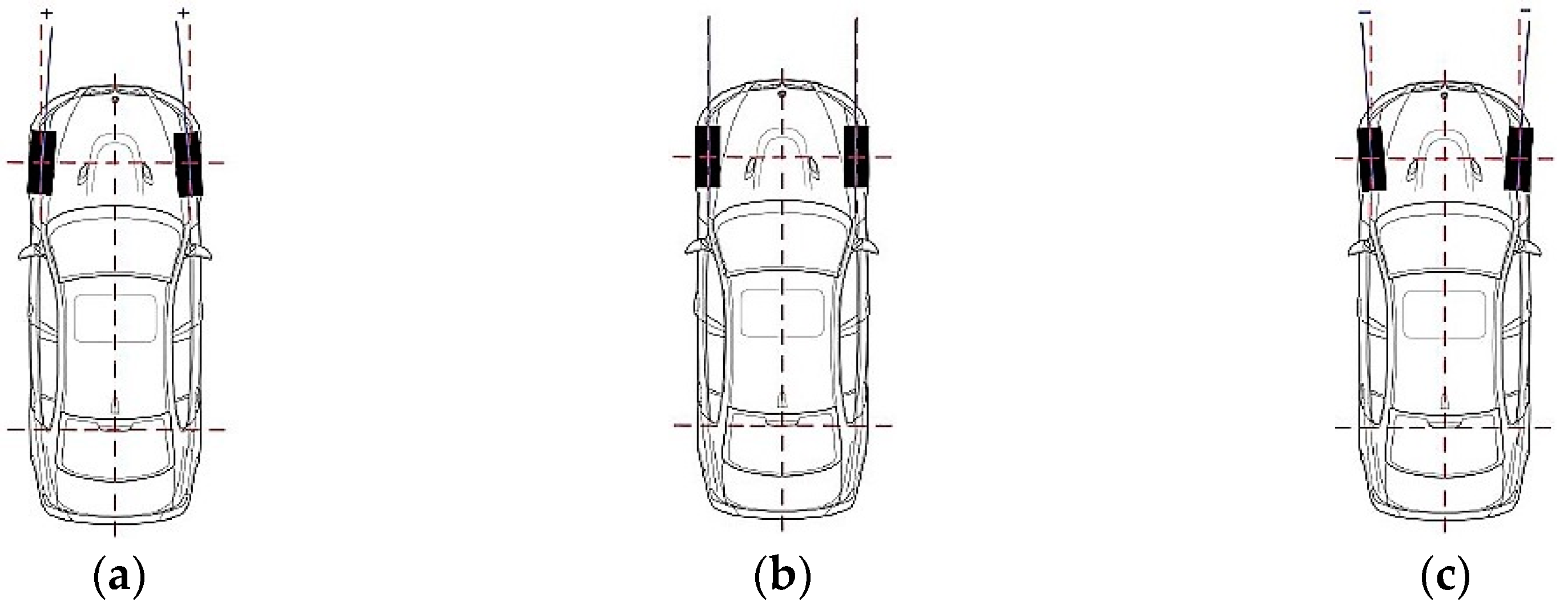
The geometry of the wheel suspension (the wheel toe—Figure 1), the wheel camber, the backward bend of the steering knuckle pivot, the turning radius of the wheel pivot, the Ackermann steering geometry are extremely important factors for designing and adjusting the wheel suspension. All of this extensively affects the driving qualities of the vehicles. The geometry can be affected by the character of the driving qualities—understeering, oversteering, the steering response, the driving comfort, etc. [11]. An appropriately designed (adjusted) geometry is able to change a non-optimal suspension (e.g., MacPherson) into a properly working unit. Its properties can even overcome a wheel suspension with a higher potential [12,13,14]. All the aforementioned aspects were analysed and included into the design of the front wheel suspension in the cross-country vehicles. However, this step was preceded by the following analysis of the current state in this area.

It is generally known that the axle is part of a vehicle through which the right and left wheels are connected with the car body. The axles of the vehicles today are relatively complicated systems from the point of view of the design. The task of this system is to ensure the best possible driving quality and driving comfort. As they are the only contact of the vehicle with the road, they extensively affect the active safety of the car. The axle connects the wheels and the bogie underframe or the car body. It transfers the gravitational, braking and inertia forces of the vehicle to the wheels. It enables an accurate and a sufficiently rigid control of the suspended wheels. As the axle is a non-suspended part of the vehicle there is an effort to implement the light metal alloys in its design as much as possible. The axles with an independent wheel suspension are made from independent half-axles—an independent wheel suspension enables a higher driving comfort. An independent wheel suspension has a stronger structure; however, it wears out more quickly. The fact they are not suitable for a difficult terrain is very important.

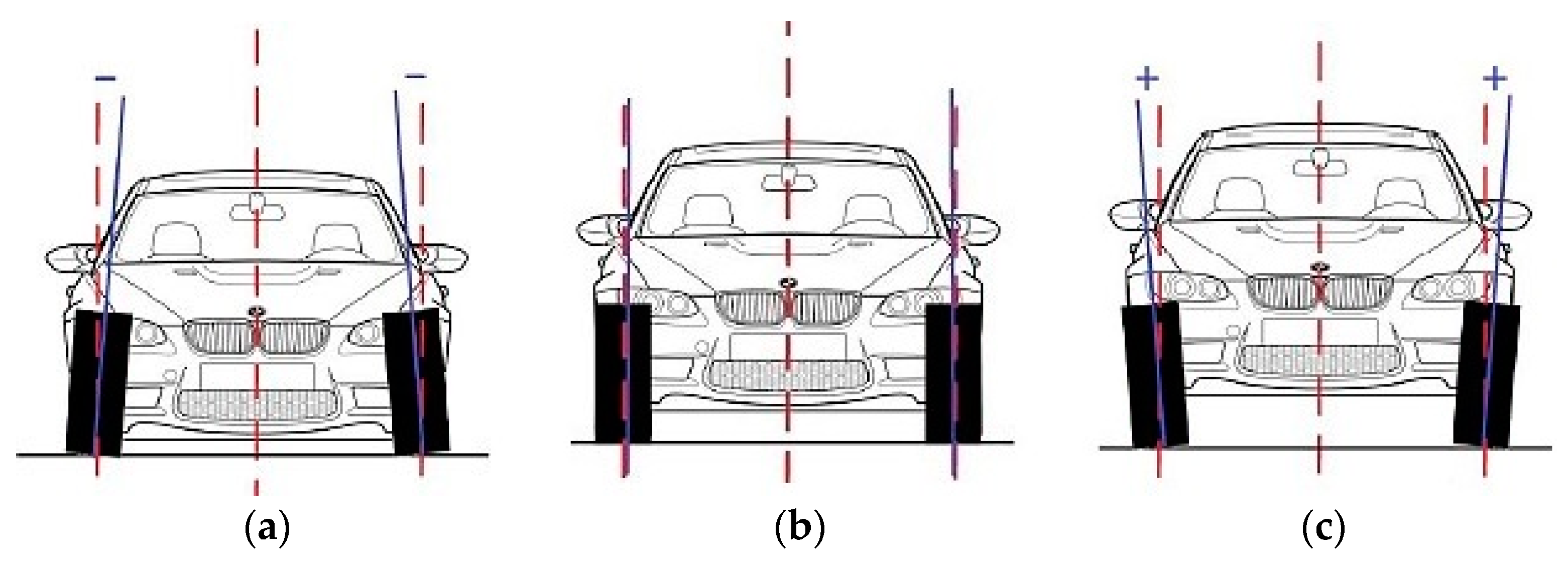
We know a double-control arms axle that is formed by an upper and bottom lateral triangular control arm. The projection of the control arms to the vertical plane is created by a trapeze. As a rule, the control arms are connected with the chassis subframe or the vehicle frame [15]. The bottom control arm has usually a more robust design due to transferring the vertical forces and a greater part of the longitudinal and lateral forces. The upper control arm is usually smaller due to the space reasons. It concerns the front axle and the place for accommodating the driving mechanism. The control arms are arranged in the rubber silent-blocks—pivot-pin bushes. The springs are usually arranged on the bottom control arm. During compression a change of the wheel camber (Figure 2), wheel toe and wheel spacing occur. This fact influences the driving quality of the vehicle negatively. An optimal control arm design and also the geometry adjustment are important for eliminating this phenomenon. Therefore, the control arms should be arranged as parallely as possible. That will cause that the wheel tilting point will be in a greater distance from the wheel. This solution reduces the wheel camber and changes the wheel spacing during compression. However, a disadvantage is the shifting of the middle of tilting of the axle to the road plane. This fact negatively influences the axis position of the vehicle´s tilting process. This changes also the angle the wheels form during the wheel compression. The position of the instantaneous point of the wheel tilt and the position of the middle of the tilt of the axle are also changed.

The double-control arm axle of an appropriate design and geometry ensures a very good wheel control. It means also very good driving properties of the vehicle. However, the relatively complicated design and higher manufacturing costs are a disadvantage of this solution. Therefore, it finds utilisation in more expensive cars. It can be used as the front driven and also driving axle and also as the rear axle. An essential disadvantage for the design of attaching the wheels of the cross-country vehicle front axle is a hard impact of the wheel towards an elevated obstacle. That is caused by the direction of the deflection of the trapezoidal control arm of the wheel suspension [15]. This direction is vertical because the spring with the damper is suspended vertically. During an impact the wheel axis passes a certain path in the direction of the car movement. This path is the same as the path of the spring shackle pin and the damper. Both the spring and the damper are compressed and the wheel suddenly accelerates to overcome the obstacle. Of course, it has an influence on the damage rate of the tyre. A rapid onset to a higher speed enormously loads the damping system of the vehicle. The maximal compression of the spring of the damper is realised in the path of the shift of the car chassis, i.e., in the path in the forward direction and equalling the wheel radius. In an ideal case, the wheels should copy the road profile and the chassis should move directly without any deviations. However, this cannot be achieved in practice. The suspension rate has to be dimensioned for the vehicle dead weight and the total weight. If the suspension rate of a particular vehicle was too high, it would not be able to absorb the unevenness. Therefore, the driving comfort and stability would be reduced. The rigid suspension, under certain circumstances, is not able to maintain the contact of the wheel with the road. And vice versa, the suspension with rigidity lower than necessary could often face bumpers. Again the driving comfort and driving properties would be deteriorated. The adjustment of the suspension rate is thus to a considerable extent a compromise [16,17].

These facts led to creating a system design for attaching the front axle wheels of a cross-country car—a buggy. The designed system is to improve the driving comfort and driving safety when the wheels overcome larger terrain obstacles. At the same time, it is desirable for the vehicle not to deteriorate the driving qualities during passing a curve and braking. The result of this effort is the described design of attaching the front axle wheels of the cross-country vehicles.

The buggy is a cross-country vehicle designed for special purposes. As a rule it is determined for one person sitting in the middle of the buggy. Although more and more hybrid drive-train are currently being used in cars, buggies are still powered by a combustion engine [18,19,20]. Such cars are produced both on the professional and amateur level. They are frequently produced individually according to the particular requirements of the user and its design utilises the already existing parts of other vehicles. As a matter of fact, it is a unique piece based on a certain scheme. It is created by a trussed frame made of steel pipes or another suitable material. The wheels are suspended independently and the axles are, as a rule, of a parallel or trapezoidal shape. The multi-element wheel suspension is also used; however, it is the most complicated one from the design point of view.

As the car is determined for racing, the issue of the driving safety is of a primary importance for its design. The system of the wheel suspension has a key influence on the driving safety [20,21]. It ensures that the car wheel provides a sufficient and optimal contact with the road (or the terrain) it is moving on. Only then it is possible to transfer the driving but especially the braking and cornering forces to the road.

2. New Design of the Wheel Suspension

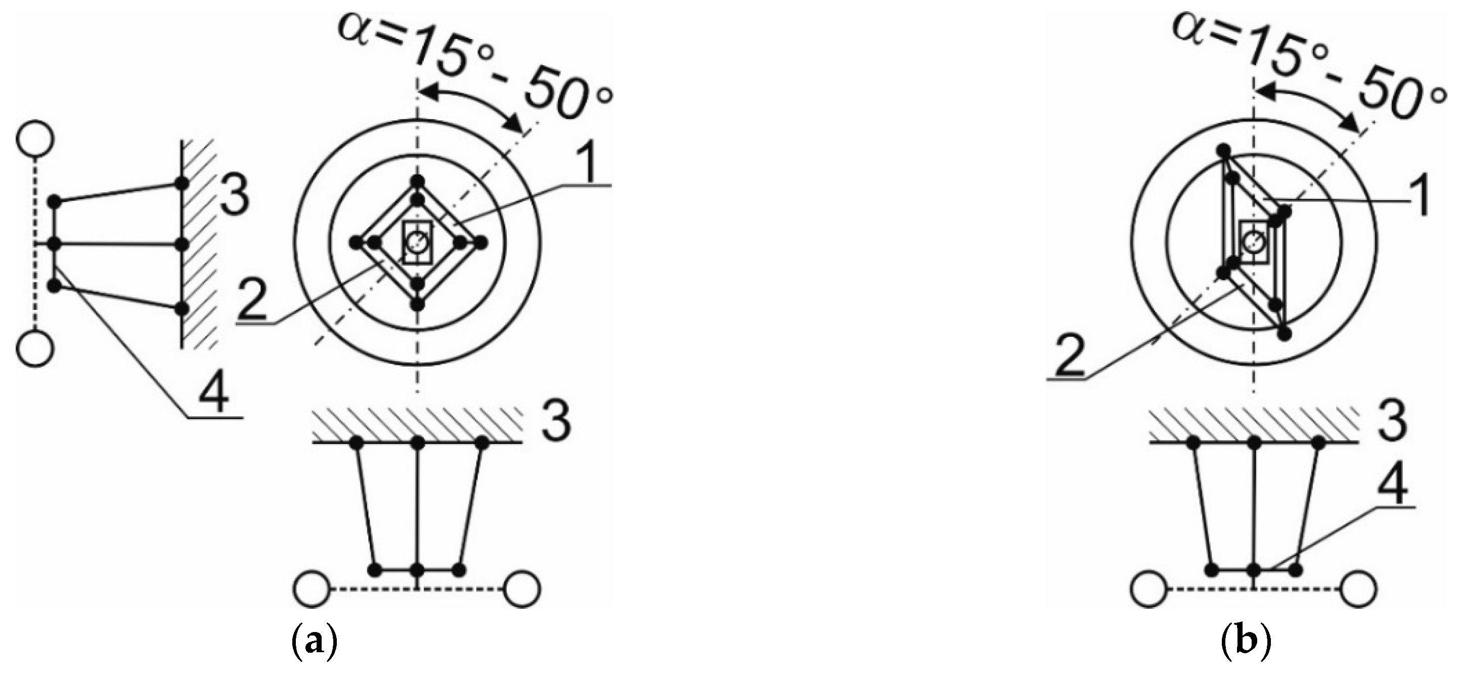
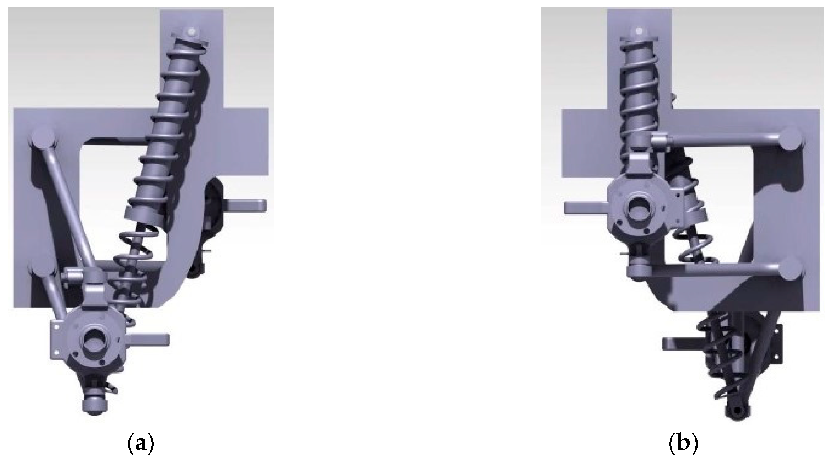
The aforementioned design shortages of the wheel suspension are removed by the design that attaches the wheels of the front axle in the cross-country vehicles according to the presented technical solution [22,23]. Its essence lies in the fact it consists of the upper (1) and bottom control arm (2). They are anchored in the basic shape of a square (SK 7960 Y1, Figure 3a) or a rhomb (SK 7945 Y1, Figure 3b) to a frame in an oscillating way and are inclined backwards by an inclination angle of α = 15° to 50° [22].

The steering knuckle pivot (4) is rotationally accommodated on the protuberant ends of the upper (1) and bottom (2) control arm. The protuberant end of the bottom control arm (2) is joined with a frame (3) through a spring (5) with the damper. If control arms are of a rhomb shape, then the steering knuckle pivot is rotationally arranged on the protuberant end of the upper control arm and on the protuberant bottom end of the control arm (Figure 3a). If both control arms are of a rhomb shape, then the steering knuckle pivots is rotationally accommodated in the middle of the protuberant upper control arm and in the middle of the bottom control arm (Figure 3b).

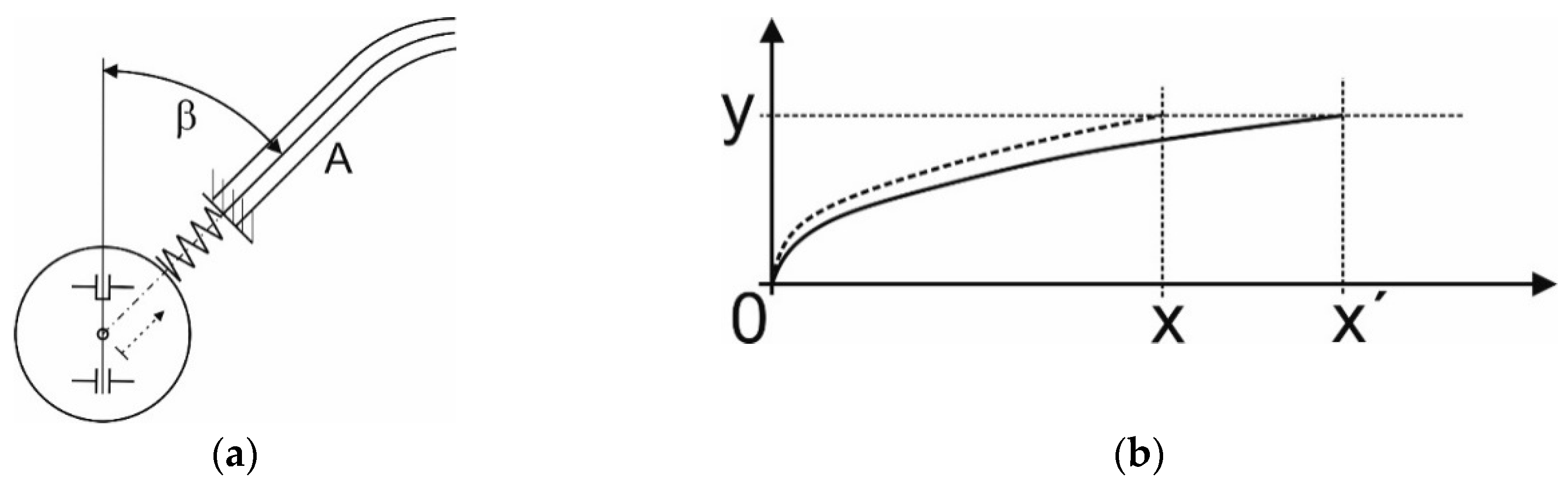
If both control arms are of a triangular shape, then the steering knuckle pivot is rotationally accommodated on the protuberant end of the upper control arm and on the protuberant bottom end of the control arm. This feature is the same for both technical solutions. The spring with the damper is oriented slantingly backwards. It is anchored in the frame by an adjustable mechanical or hydraulic member. The camber of anchoring from the vertical axis is in the range of β = 10° to 60°. It is advantageous if the spring with the damper is oriented in the direction towards the A column of the vehicle frame. 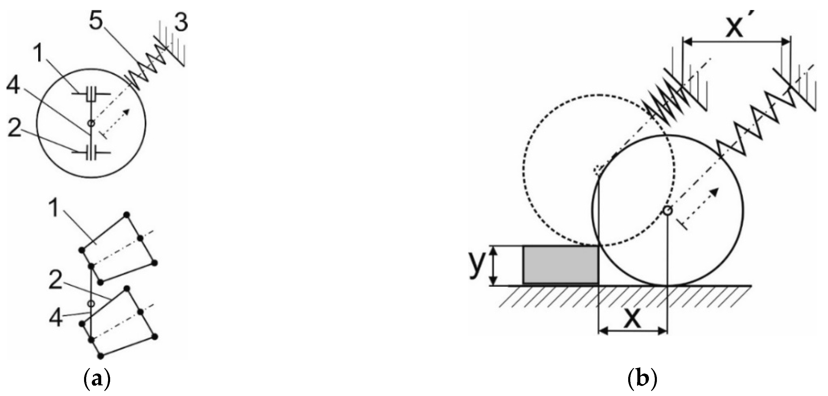Figure 4a schematically depicts the arrangement kinematics of the wheel attachment design with the spring. Figure 4b presents the function of the design [22].

The advantages of the design of attaching the front axle wheel in the cross-country vehicles according to the technical solution presented are apparent on the basis of its effects. The effects consist in the fact that it is possible to increase the speed of the car and to overcome higher terrain obstacles as well. It is achieved by a more continuous raid against the obstacle and it improves the comfort of the car crew. The car structure is also not loaded as much. During the front-end impact against an obstacle the second ends of the spring with the damper and anchoring pivot are anchored in the direction of the column A of the car frame. The impact force of the wheel is then transferred to the column A. Therefore, this set fulfils the function of a damper. The secondary advantages of the solution consist in lower wear of the tyres, gear box and engine. If it is possible to change the point of the strut of the absorber attachment on the vehicle frame (in leaps or continuously), then it is possible to change actively the undercarriage ride height. This enables to select the driving regime e.g., on the highway with a low undercarriage ride height or in the terrain with a high undercarriage ride height. Figure 5a shows the direction of the impact forces to the column A.

Figure 3, Figure 4 and Figure 5 depict these utility models and are of a documentation character. They graphically show what effects of the design the authors expect.

Figure 5b depicts a gradual run-up on an obstacle. When the wheel runs on an obstacle its motion has to be equal with height of the obstacle (Figure 5b, the vertical axis y). The presented solution will cause a motion of the wheel on a part of the circle. Therefore, its motion will last a longer time (Figure 5 because the path of the wheel will prolong). This fact will affect the passengers´ comfort. From the physical point of view, we expect a smaller vertical acceleration on the passengers. And this is the biggest benefit of this design. After the acceptation of the technical solution by the authorities the authors continue creating its 3D CAD model.

3. Creating A 3D Model of the Wheel Suspension and Its Modification

Based on the previous analysis we created a 3D model of suspending the front wheels of a cross-country vehicle. It is a suspension with an upper and bottom control arm. These control arms are tilted backwards in the longitudinal direction. In the protuberant ends of the control arms there is a rotationally accommodated steering knuckle pivot. At the same time a damper is attached in the protuberant end of the bottom control arm. It is attached to the car frame on the opposite end. In this way the wheel carries out a compound motion. It is created by a motion upwards and at the same time a motion backwards, i.e., it is a motion along part of a circle. This enables a better absorption of unevenness of the road and this fact enables the car to be more comfortable and controllable. Simultaneously the suspension components are loaded less as well. It is an independent wheel suspension.

Thanks to this design there will be no change of the wheel camber, the steering pivot back-bend or wheel spacing. This is the main advantage in comparison with the conventional suspension types. It will be suitable to follow this assumption by the sensitivity analysis. From the point of view of geometry only a change of the wheel toe occurs. But this is inevitable in the case of an independent wheel suspension. On the other hand, the suspension motion will cause a larger wheel base. The design will be implemented in the cars with a relatively high stroke and therefore it is suitable to complete it by a device for a continuous change of the clear height. It means that the car is able to maintain a large clear height in the terrain. It guarantees better overhang and breakover angles of the chassis and a better passability over the terrain unevenness [24,25]. The undercarriage height can be lowered during the drive on a road. This will lower the vehicle centre of gravity (CoG) and the controllability of the car will be improved. If necessary, the height of each wheel can be adjusted separately. This solution is suitable for improving the vehicle passability over an inclined plane. This concerns both the transverse and longitudinal direction.

This section may be divided by subheadings. It should provide a concise and precise description of the experimental results, their interpretation as well as the experimental conclusions that can be drawn.

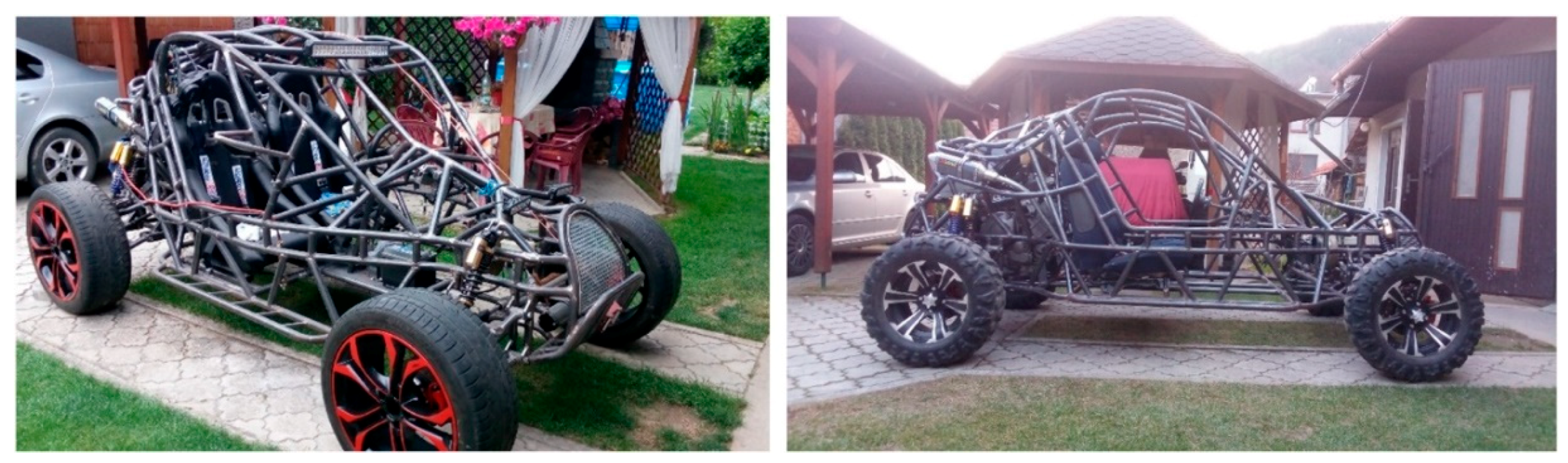
First of all, it was necessary to determine for which vehicle this wheel suspension should be dimensioned. The authors chose a buggy prototype, as shown in Figure 6, with known technical data, as shown in

Table 1. Technical parameters of the vehicle considered.

Parameter	Indication	Value	Unit
maximal weight	mmax	780	kg
wheel width	a	245	mm
wheel radius	r	376	mm
wheelbase of wheel axes	z	2350	mm
Spacing of wheel axes	o	1500	mm
vehicle dead weight	mp	640	kg
considered load of the front axle	m	300	kg
perpendicular distance of control arms joints	i	300	mm
designed weight of control arm	mkr	6	kg
designed weight of vertical control arm	mzr	3.45	kg
weight of wheel body (8E0501611J)	mnk	3.28	kg
total weight of non-suspended material belonging to one wheel	mN	5.35	kg
weight wheel journal	mc	6.1	kg

. This vehicle is suitable for this type of suspension. The car is able to drive relatively fast on the road but also in heavy off-road conditions. It is a buggy with a welded pipe frame, with a motor in the rear part and a back-wheel drive.

The following requirements were taken into account:

• The possibility of geometry adjustability and suspension rate in the largest possible range.
• The suspension must be rigid enough to fulfil the safety requirements in operation.
• The suspension must not be more rigid than the vehicle frame.
• The life span and manufacturing costs.

During creating the 3D model according to SK 7945 Y1 and SK 7960 Y1 [18,19] we found out that this solution would not enable adjusting the camber and back-bend of the vertical steering axis. The original design counted with arranging the vertical pivot rotationally in the protuberant ends of the upper and the bottom control arm. 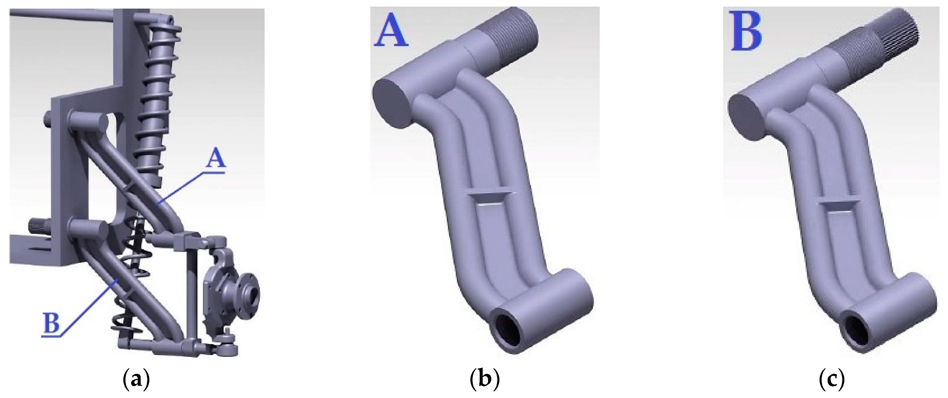The arrangement of the vertical steering pivot is therefore one of the most principal changes of the modified solution (Figure 7a). The suspension with a separated axis of rotation was used for achieving the possibility to adjust the camber and back-bend of the vertical steering axis. It resembles the MacPherson system with a separated axis of rotation. The advantage of this solution is that smaller inertia forces perform on steering. Therefore, the feedback of the steering system will be less affected. The control arms also underwent adaptations. The original system contained control arms created by one pipe. After modification each control arm is created by two pipes placed next to each other. Such a solution positively affects the load during passing a curve. The control arms are bent twice towards the vehicle frame. This will ensure a sufficient angle of the wheel rotation. If a torsion stabiliser was used, both bottom control arms would be equipped with a spline shaft.

The control arm (Figure 7b,c) is 350 mm long (the perpendicular distance between attachments) and 284 mm wide (the distance between the assembly surfaces). The bottom control arm has an attachment of the torsion stabiliser. The attachment of the vertical control arm is welded on the opposite end of the control arm. The control arm consists of two bent pipes. A steel plate is welded between the pipes which strengthens the control arm structure. We used the material—steel 25CrMo4. This steel is used for manufacturing roll cages of the racers and other heavily loaded structures. The yield strength achieves 590 MPa.

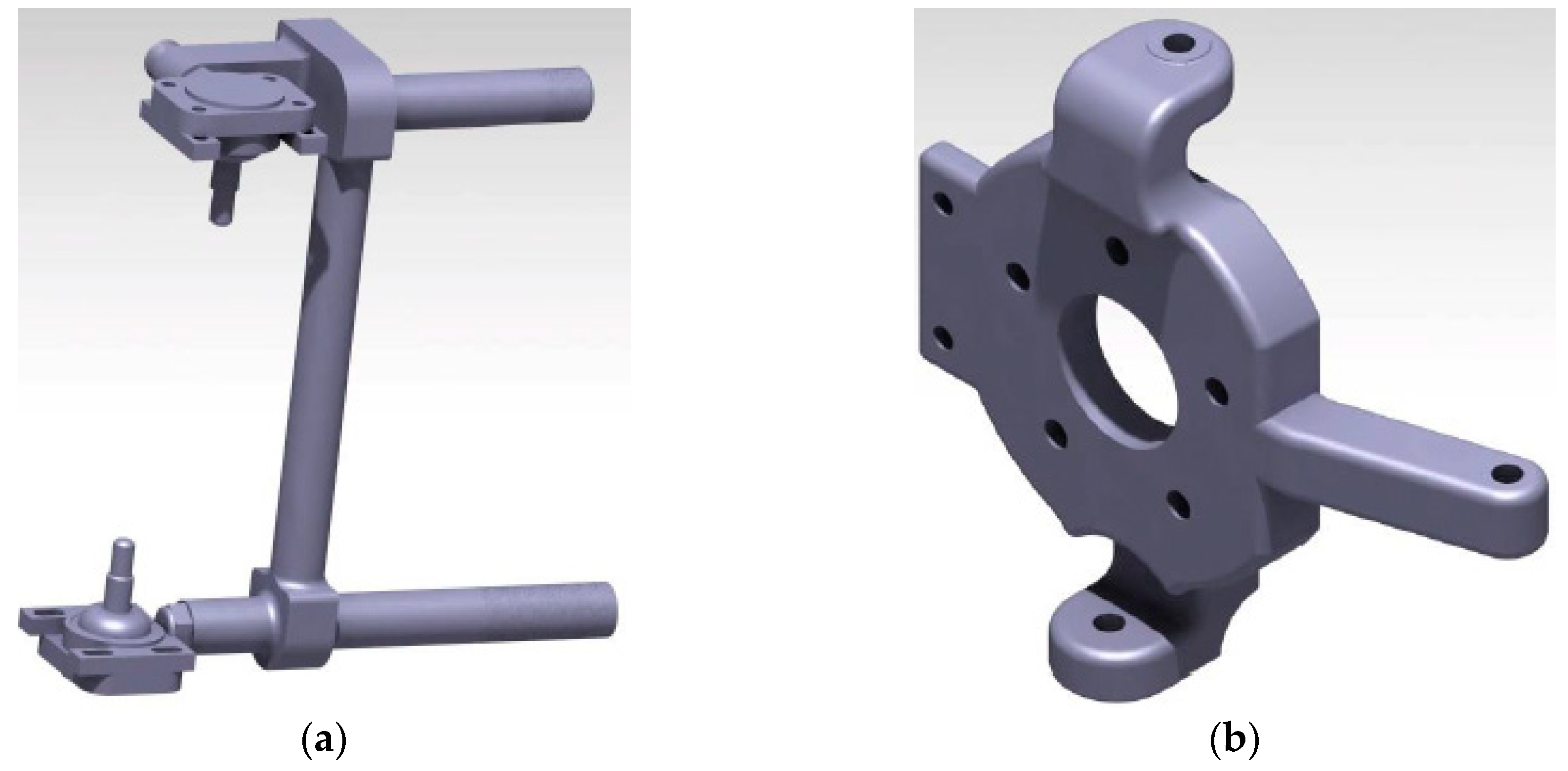
The vertical control arm (Figure 8a) joins the control arms and at the same time it creates a base for the separated axis of rotation. On the internal side of the control arm we can find pivots which attach the vertical control arm to the control arms. On the external part there are assembly points for the knuckle bolts. The assembly point for the upper knuckle bolt is oriented longitudinally which will enable changing the back-bend of the steering axis. The back-bend can be adjusted by screwing the attachment of the knuckle bolt to the required distance. Its position will be horizontal and then the adjustment of the accurate angle will be possible by using the eccentric knuckle bolt. The bottom attachment is oriented transversely. This will enable adjusting the wheel camber in the same way. The difference consists in the fact that the bottom knuckle bolt is pressed in the flange. The flange can be screwed to the attachment of the knuckle bolt. The material for the vertical control arm is the steel 25CrMo4 with the yield strength of R_e = 590 MPa.

The wheel pivot bolt (Figure 8b) is connected with the vertical control arm by the upper and bottom knuckle bolts. The design will enable using the brake callipers of various sizes depending on the requirements. On the pivot bolt there is an attachment for the steering pivot. The design of the wheel suspension will also ensure a suitable Ackermann steering geometry. The material of the pivot bolt is the grey cast iron with the yield strength of 500 MPa.

As it is a suspension with a relatively high stroke (the mechanism kinematics—Figure 9—enables a stroke of up to 150 mm) the change of the wheel toe during the suspension motion will be also relatively large. In the case of using the vehicle mainly with a big clear height the wheel toe value of 0° to −0.1° is suitable. This is caused by the fact that due to compressing the suspension the wheel toe will change to positive values. If the vehicle is used with a lower clear height, the wheel toe value of approximately 0.2 degree is suitable. The reason for this is that a change of the wheel toe to a negative value develops during loading off the suspension.

For the purposes of the finite element analysis of the designed suspension it is necessary to determine the forces performing on the suspension. These forces are to be determined in selected driving situations. The driving situations result from the car operation. It is a very demanding thing to cover all the variations of the driving situations. Out of all possibilities the car can encounter in operation, the most frequent and important ones for the selected vehicle will be chosen. They will be - turning at the edge of adhesion, maximal braking action and driving in terrain with the maximal crossing of the axles. These three driving situations will cover the forces performing in the transverse, longitudinal and vertical direction.

4. Analysis of Load Forces

Turning at the edge of adhesion is a driving situation when the car turns at the maximal lateral overload. The vehicle achieves the adhesion limit and in dependence on the car type it starts sliding outwards. The sliding movement can be caused by an oversteering or understeering slide of the front axle. In some cases, a lateral slide of both axles can develop. The understeering slide is simpler to cope with by a common user. Therefore, the majority of the series cars are adjusted for the limit values of the understeering slide. To cope with the understeering slide, it is necessary to load the front wheels for them to acquire the necessary traction. The simplest way is to throttle back gradually or in some situations (mainly the cars with a lighter front axle) to slow down softly. This operation will not block the wheels. This is the case of our vehicle. It has the weight distribution in favour of the rear axle. It means when we gradually approach the edge of adhesion it will behave in an understeering way.

During calculations it is suitable to work with the maximal total weight of the car. The weight of the maximally loaded front axle is 290 kg. For the safety purposes, we will work with the axle load of m = 300 kg.

Firstly, forces acting on a suspension during driving in straight direction have had to be quantified. Calculation of the force loading a wheel is given as following (1):

$$F_Z=\frac{G_O}{2}+G_N,$$

(1)

where G_O (N) is the gravitational force of the sprung weight for the front axle and G_N (N) is the gravitational force of the unsprung weight for the wheel.

The weight of the unsprung axle parts (control arms, spring, damper, silent-blocks, vertical control arm, steering knuckle of the wheel, wheel hub, pivot-pin bush, wheel and tyre) is m_N = 58.32 kg per one wheel. Then the equation for the gravitational force of the unsprung components is as follows (2):

$$G_N=m_N·g,$$

(2)

where m_N (kg) is the weight of the unsprung axle parts per one wheel, g (m·s⁻²) is the constant of the gravitational acceleration. Thus,

$$G_N=m_N·g=58.32·9.81=572.12N,$$

(3)

The gravitational force of the unsprung weight per the front axle (3):

$$\begin{array}{l}{G}_O=\left(m-2·m_N\right)·g,\\ G_O=\left(m-2·m_N\right)·g=\left(300-2·58.32\right)·9.81=1800N.\end{array}$$

(4)

The static force loading the wheel according to the Equation (1) will be:

$$F_Z=\frac{G_O}{2}+G_N=\frac{1800}{2}+572.12=1472.12N,$$

(5)

During driving the value of the static force is changed and reaches its minimum and maximum. Therefore it is necessary to define the maximal force that depends on the camber rate (4):

$$F_{Z_{\max }}=F_Z·k,$$

(6)

where k (-) is the dynamic coefficient depending on the camber rate k = 1.8 (-) [26],

$$F_{Z_{\max }}=F_Z·k=1472.12·1.8=2650N.$$

(7)

Then we will calculate the lateral transverse force during a curved track run. For this case the additional load of the wheel in a vertical direction will not be greater than the load due driving in terrain with the maximal crossing of the axles. Due to this fact it is sufficient to carry out the FEM analysis only for driving in terrain with the maximal crossing of the axles. The calculation of the theoretical maximal centrifugal force at the adhesion limit (8) is as follows:

$$F_O=F_1·{\mu }_p,$$

(8)

where F₁ (N) is the gravitational force for the front axle being solved determined by the equation (9), μ_p (-) is the tyre adhesion coefficient, we consider μ_p = 0.925 (-),

$$\begin{array}{l}{F}_1=m·g,\\ F_1=m·g=300·9.81=2943N,\end{array}$$

(9)

$$F_O=F_1·{\mu }_p=2943·0.925=2722.3N.$$

(10)

During a curved track run the forces on the external and internal tyre are different. The tyre on the outer side is loaded by a substantially larger transverse force. Let us carry out a calculation of the difference of the transverse force between the external and internal tyre. It is valid for the unsprung weight per one axle (11):

$$\mathsf{\Delta }{F}_{ZO}=\frac{G_O}{B}·{\mu }_p·h_t,$$

(11)

where B (m) is the wheel spacing, B = 1.62 m, h_t (m) is the height of the CoG of the unsprung masses, h_t = 0.8 m,

$$\mathsf{\Delta }{F}_{ZO}=\frac{G_O}{B}·{\mu }_p·h_t=\frac{1800}{1.62}·0.925·0.8=825N.$$

(12)

For the unsprung weight per one axle it is valid (13):

$$\mathsf{\Delta }{F}_{Zn}=\frac{G_N}{B}·{\mu }_p·h_n,$$

(13)

where h_n (m) is the height of the CoG of the unsprung masses, h_n = 0.352 m,

$$\mathsf{\Delta }{F}_{Zn}=\frac{G_N}{B}·{\mu }_p·h_n=\frac{572.12}{1.62}·0.925·0.352=115N.$$

(14)

The transverse force of the external and internal tyre (15):

$$\begin{array}{l}\mathsf{\Delta }{F}_Z=\mathsf{\Delta }{F}_{ZO}+\mathsf{\Delta }{F}_{Zn},\\ \mathsf{\Delta }{F}_Z=\mathsf{\Delta }{F}_{ZO}+\mathsf{\Delta }{F}_{Zn}=825+115=940N.\end{array}$$

(15)

The calculation of the maximal lateral transverse force performing on the tyre of the external wheel (16):

$$\begin{array}{l}\mathsf{\Delta }{F}_{y1}=\left(F_{z_{\max }}+\mathsf{\Delta }{F}_z\right)·{\mu }_p,\\ \mathsf{\Delta }{F}_{y1}=\left(F_{z_{\max }}+\mathsf{\Delta }{F}_z\right)·{\mu }_p=\left(2650+940\right)·0.925=3325N.\end{array}$$

(16)

The calculation of the maximal lateral transverse force performing on the tyre of the internal wheel (17):

$$\begin{array}{l}\mathsf{\Delta }{F}_{y2}=\left(F_{z_{\max }}-\mathsf{\Delta }{F}_z\right)·{\mu }_p,\\ \mathsf{\Delta }{F}_{y2}=\left(F_{z_{\max }}-\mathsf{\Delta }{F}_z\right)·{\mu }_p=\left(2650-940\right)·0.925=1585N.\end{array}$$

(17)

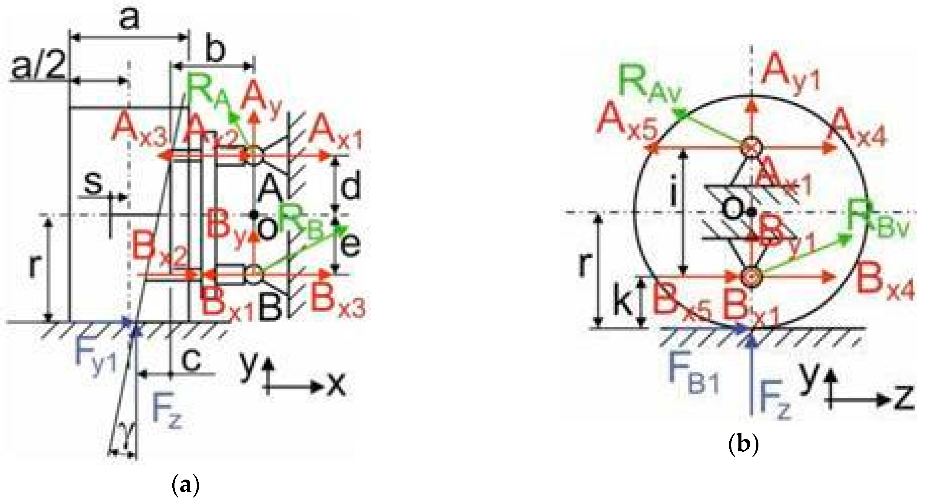
It is necessary to use the release method (Figure 10a) for calculating the forces loading the wheel suspension and in this way to set up the conditions of equilibrium.

We will use the superposition method, i.e., the force effects of each force will be investigated separately. There are two loading forces during a curved track run (Figure 10a—in blue colour)—F_z and F_y1. The force F_z forms a displacement effect to the links A, B. We assume a uniform division of this force between the links A and B. Therefore, the reaction effects develop—Figure 10a in red colour - A_y and B_y. Their values are detected through the exception of the equilibrium (18) respecting the vector algebra:

$${\displaystyle \sum _i{F}_{iy}=0\Rightarrow A_y+B_y-F_z=0}.$$

(18)

As this is an equation in two unknowns, the second condition will be determined under an assumption of a uniform division of the force displacement effect (19):

$$A_y=B_y.$$

(19)

Through implementing the Equation (19) into the Equation (18) and entering corresponding values we will achieve:

$$\begin{array}{l}{A}_y=736.06N,\\ B_y=736.06N.\end{array}$$

(20)

The force F_z also continues loading the suspension by a rotational effect. The goal is to quantify the reaction force effects in the links A and B. In the geometrical centre of the links A and B, a point O was created, as Figure 10a shows. The torque of the force F_z to this point is (32):

$$\begin{array}{l}{M}_{k1}=F_z·\left(b+c\right),\\ M_{k1}=1472.12·\left(381+92\right)=696312.76N·mm\end{array}$$

(21)

This torque effect will be replaced by a couple of forces arousing an equivalent torque. Therefore, Figure 10a shows the reactions A_x1 and B_x1 (in red colour). As they have the same distance from the point O, we can calculate them as follows (22):

$$M_{k1}=A_{x1}·d+B_{x1}·e,$$

(22)

or also (23):

$$\begin{array}{l}{M}_{k1}=A_{x1}·i,\\ A_{x1}=\frac{M_{k1}}{i}=\frac{696312.76}{300}=2321N=B_{x1}.\end{array}$$

(23)

The force F_y1 creates a displacement effect to the considered links (A, B). We assume a uniform division of this force between the links A and B. Therefore, the reaction effects (Figure 10a—in red colour) A_x2 and B_x2 will develop. Their values will be detected by an equilibrium exception (24):

$${\displaystyle \sum _i{F}_{ix}=0\Rightarrow A_{x2}+B_{x2}-F_{y1}=0}.$$

(24)

As it is an equation in two unknowns, the second condition will be determined under the assumption of a uniform division of the force effect (25):

$$A_{x2}=B_{x2}.$$

(25)

Through implementing the Equation (25) into the Equation (24) and entering corresponding values we will achieve:

$$\begin{array}{l}{A}_{x2}=1662.5N,\\ B_{x2}=1662.5N.\end{array}$$

(26)

The force F_y1 also continues loading the suspension by a rotational effect. The goal is to quantify the reaction force effects in links A and B. In the geometrical centre of the links A and B, a point O was created, as Figure 10a shows. The torque of the force F_y1 to this point are (27):

$$\begin{array}{l}{M}_{k2}=F_{y1}·r,\\ M_{k2}=3325.376=1250200N·mm\end{array}$$

(27)

This torque effect will be replaced by a couple of forces arousing an equivalent torque. Therefore, Figure 10a shows the reactions A_x3 and B_x3 (in red colour). As they have the same distance from the point O, we can calculate them as follows (28):

$$M_{k2}=A_{x3}·d+B_{x3}·e,$$

(28)

or also (29):

$$\begin{array}{l}{M}_{k2}=A_{x3}·i,\\ A_{x3}=\frac{M_{k2}}{i}=\frac{1250200}{300}=4167N=B_{x3}.\end{array}$$

(29)

The resulting force in the joint A in the x direction will be (30):

$$\begin{array}{l}{A}_x=A{}_{x1}+A_{x2}-A_{x3},\\ A_x=2321+1662.5-4167=-183.5N.\end{array}$$

(30)

The resulting force in the joint A in the y direction will be (31):

$$A_y=736.06N.$$

(31)

The resulting force loading the joint A (Figure 10a—green R_A) will be (32):

$$\begin{array}{l}{R}_A=\sqrt{A_x^2+A_y^2},\\ R_A=\sqrt{{\left(183.5\right)}^2+{\left(736.06\right)}^2}=760N.\end{array}$$

(32)

The resulting force in the joint B in the x direction will be (33):

$$\begin{array}{l}{B}_x=B{}_{x3}+B_{x2}-B_{x1},\\ B_x=4167+1662.5-2321=3510N.\end{array}$$

(33)

The resulting force in the joint B in the y direction will be (34):

$$B_y=736.06N.$$

(34)

The resulting force loading the joint B (Figure 10a—green R_A) will be (35):

$$\begin{array}{l}{R}_B=\sqrt{B_x^2+B_y^2},\\ R_B=\sqrt{{\left(3510\right)}^2+{\left(736.06\right)}^2}=3590N.\end{array}$$

(35)

According to the calculation a planar force of R_B = 3590 N affects the suspension through the pivot joint. It is oriented towards the vehicle frame in the place of suspension of the bottom knuckle bolt. In the place of suspension of the upper knuckle bolt there is a planar force of R_A = 760 N.

Table 2. Geometrical parameters of the analytical calculation.

Quantity	Value
a	245 mm
b	381 mm
c	92 mm
d	150 mm
e	150 mm
i	300 mm
k	226 mm
r	376 mm
s	32 mm
γ	17°

gives the values of the geometrical parameters from Figure 10.

During maximal deceleration a large part of the total weight will affect the front axle of the vehicle. The coefficient for loading the front axle of k_b = 1.4 (-) is suitable for the reference vehicle (a buggy with a rear engine and distribution of the weight in favour of the rear axle). The load of the front axle during deceleration of the vehicle will be (36):

$$\begin{array}{l}{F}_{z1B}=F_1·k_b,\\ F_{z1B}=2943·1.4=4120.2N.\end{array}$$

(36)

In the contact area of the wheel with the road there are forces necessary for quantifying the effects on the suspension. The calculation of the force performing in the contact area of the wheel with the road (37):

$$\begin{array}{l}{F}_{B1}=F_{z1B}·{\mu }_p,\\ F_{B1}=4120.2·0.925=3811.185N.\end{array}$$

(37)

It is necessary to use the release method (Figure 10a) for calculating the forces loading the wheel suspension and in this way to set up the conditions of equilibrium. We will use the superposition method, i.e., the force effects of each force will be investigated separately. There are two loading forces during a curved track run (Figure 10a—in blue colour)—F_z and F_B1. The force F_z forms a displacement effect to the links A, B. We assume a uniform division of this force between the links A and B. Therefore, the reaction effects develop—Figure 10a in red colour—A_y and B_y. Their values are detected through the exception of the equilibrium (38):

$${\displaystyle \sum _i{F}_{ix}=0\Rightarrow -A_y-B_y+F_z=0}.$$

(38)

As it is an equation in two unknowns, the second condition will be determined under the assumption of a uniform division of the force displacement effect (19):

$$A_y=B_y.$$

(39)

Through implementing the Equation (39) into the Equation (38) and entering corresponding values we will achieve:

$$\begin{array}{l}{A}_y=736.06N,\\ B_y=736.06N.\end{array}$$

(40)

The force F_z continues loading the suspension also by a rotational effect. It is not necessary to calculate this load because it is the same load as in the previous case (Ax₁, Bx₁). The force F_B1 creates a displacement effect to the links (A, B). We assume a uniform distribution of this force between the links A and B. Therefore, the reaction effects (Figure 10b—in red colours) A_x4 a B_x4 develop. Their values are detected by an exception from the equilibrium (41):

$${\displaystyle \sum _i{F}_{iz}=0\Rightarrow A_{x4}+B_{x4}-F_{B1}=0}.$$

(41)

As it is an equation in two unknowns, the second condition will be determined under the assumption of a uniform distribution of the force displacement effect (42):

$$A_{x4}=B_{x4}.$$

(42)

Through implementing the Equation (42) into the Equation (41) and entering corresponding values we will achieve:

$$\begin{array}{l}{A}_{x4}=1905.5N,\\ B_{x4}=1905.5N.\end{array}$$

(43)

The force F_B1 continues loading the suspension also by a rotational effect. The goal is to quantify the reaction force effects in the links A and B. In the geometrical centre of the links A and B a point o (Figure 10b) was created. The torque of the force F_B1 to this point will be (44):

$$\begin{array}{l}{M}_{k3}=F_{B1}·r,\\ M_{k3}=3811.185·376=1433005.56N·mm.\end{array}$$

(44)

This torque effect will be replaced by a couple of forces arousing an equivalent torque. Therefore, Figure 10b shows the reactions A_x5 and B_x5 (in red colour). As they have the same distance from the point O, we can calculate them as follows (45):

$$M_{k3}=A_{x5}·d+B_{x5}·e,$$

(45)

or also (46):

$$\begin{array}{l}{M}_{k3}=A_{x5}·i,\\ A_{x5}=\frac{M_{k3}}{i}=\frac{1432935.56}{300}=4776.4518\overline{6}N.\end{array}$$

(46)

The resulting force in the joint A in the z direction will be (47):

$$\begin{array}{l}{A}_{xv}=-A_{x5}+A_{x4},\\ A_{xv}=-4776.452+1905.5=-2870.952N.\end{array}$$

(47)

The resulting force in the joint A in the y direction will be (48):

$$A_{y1}=736.06N.$$

(48)

The resulting force loading the joint A (Figure 10b—green R_Av) will be (49):

$$\begin{array}{l}{R}_{Av}=\sqrt{A_{xv}^2+A_{y1}^2+A_{x1}^2},\\ R_{Av}=\sqrt{{\left(2871\right)}^2+{\left(736.06\right)}^2+{\left(2321\right)}^2}=3765N.\end{array}$$

(49)

The resulting force in the joint B in the z direction will be (50):

$$\begin{array}{l}{B}_{xv}=B_{x5}+B_{x4},\\ B_{xv}=4776+1905.5=6681.5N.\end{array}$$

(50)

The resulting force in the joint B in the y direction will be (51):

$$B_y=736.06N.$$

(51)

The resulting force loading the joint B (Figure 10b—green R_Bv) will be (52):

$$\begin{array}{l}{R}_{Bv}=\sqrt{B_{xv}^2+B_{y1}^2+B_{x1}^2},\\ R_{Bv}=\sqrt{{\left(6681.5\right)}^2+{\left(736.06\right)}^2+{\left(2321\right)}^2}=7111N.\end{array}$$

(52)

According to the calculation a space force of R_Bv = 7111 N affects the suspension through the pivot joint. It is oriented towards the vehicle frame in the place of suspension of the bottom knuckle bolt. In the place of suspension of the upper knuckle bolt there is a space force of R_Av = 3765 N.

For the finite element analysis (Section 5) it is inevitable to know the value of the load force of the analysed control arm during passing a curve. The calculation of the necessary quantities will be carried by an analytical calculation. Our calculation is based on the force distribution in the wheel suspension depicted in Figure 10.

5. Static FEM Analysis and Modal Analysis of Designed Components for Individual Driving Regimes

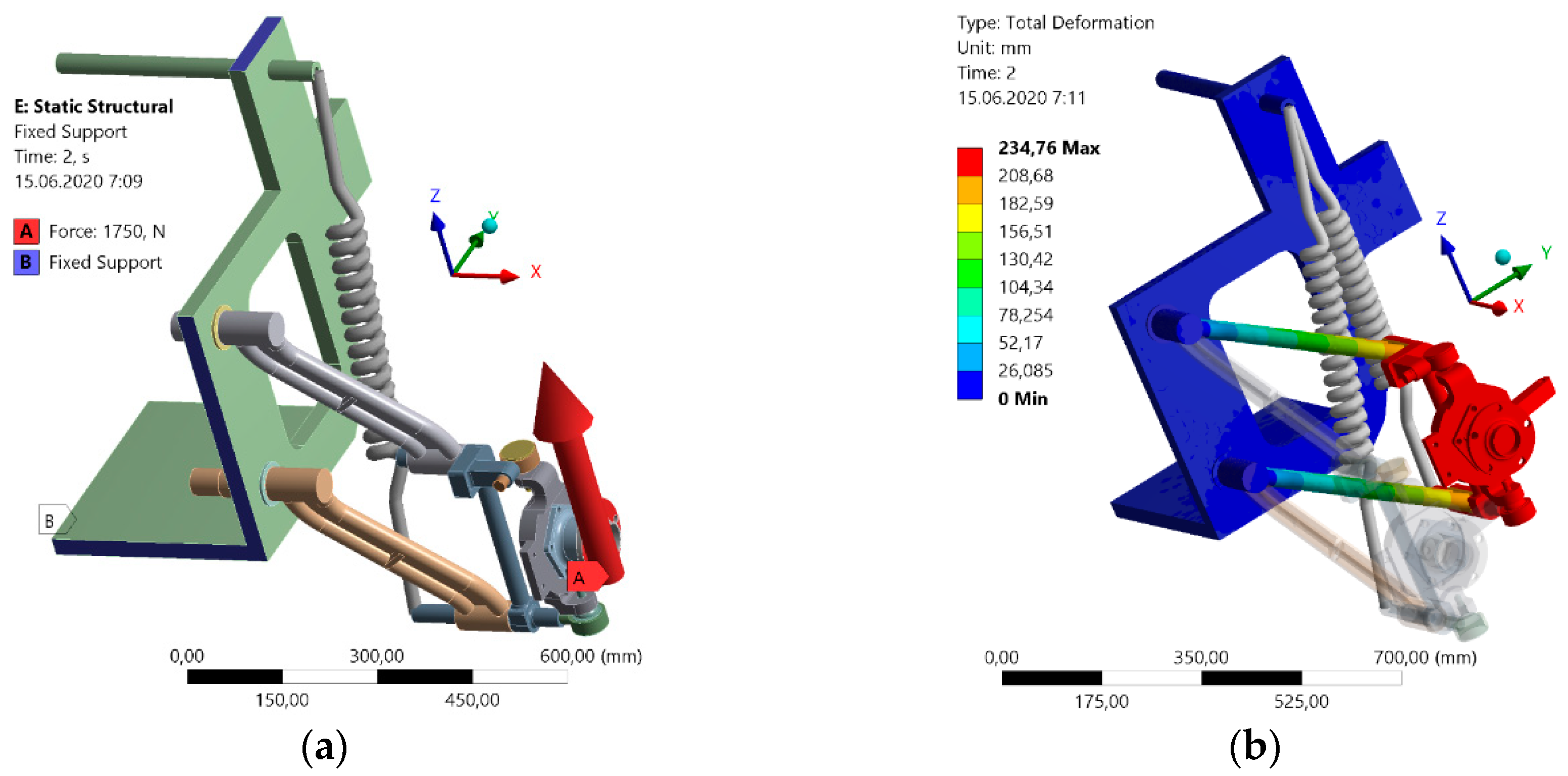
First of all, we realised a static analysis of the car suspension. We investigated the distribution of the stresses in the main suspension parts for a free standing vehicle. We considered the wheel force of 1750 N (Figure 11a). It is by 18% more (1472.12 N) than the wheel force defined in the analytical way according to the Equation (1). This calculation is only of an informative character. Of course, the dynamic load of the vehicle will be higher. However, it is possible to observe the value of the shift (Figure 11b) from the car self-weight. This parameter can be regulated through changing the spring force and the damping coefficient. Due to the symmetry of the axle it was possible to with a half of the model.

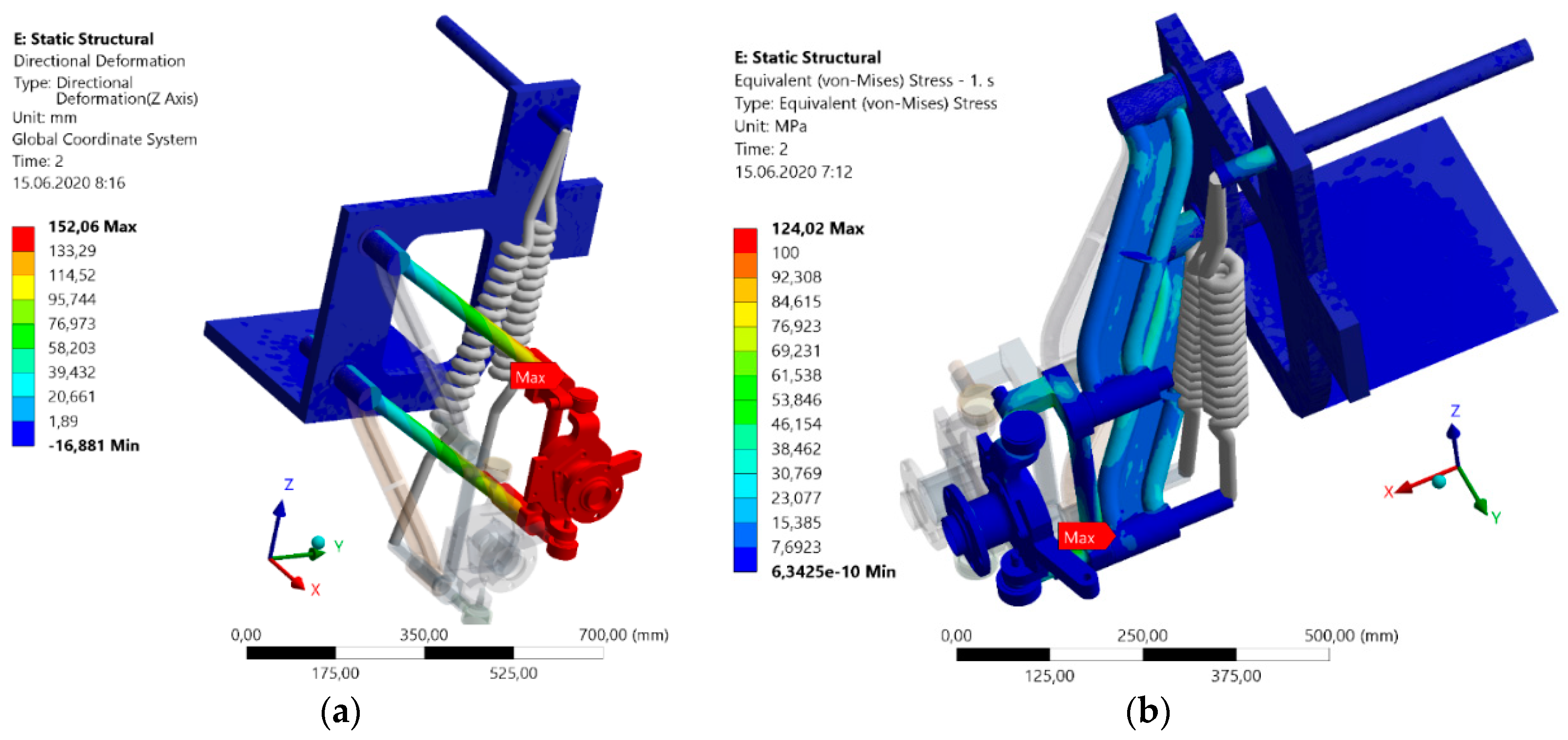
The analysis result shows that the overall shift of the wheel will be 234.76 mm. This value id changeable, it will be suitable to make this mechanism with a possibility of the automatic regulation. Only in this way we will ensure the optimal utilisation of its potential. The authors plan to compare their solution with other convectional suspensions (Section 6 dealing with the sensitivity analysis). Therefore, they present also the results of the shift analysis only in the vertical direction (Figure 12a). Just this solution indicator is the same both for our and other commercial wheel suspensions.

The authors were also interested in the stress distribution in the suspension parts for a standing car (Figure 12b). The boundary conditions for this calculation are presented in Figure 11a. The material characteristics of individual components are described in the next text. The maximal analysed stress was 124 MPa.

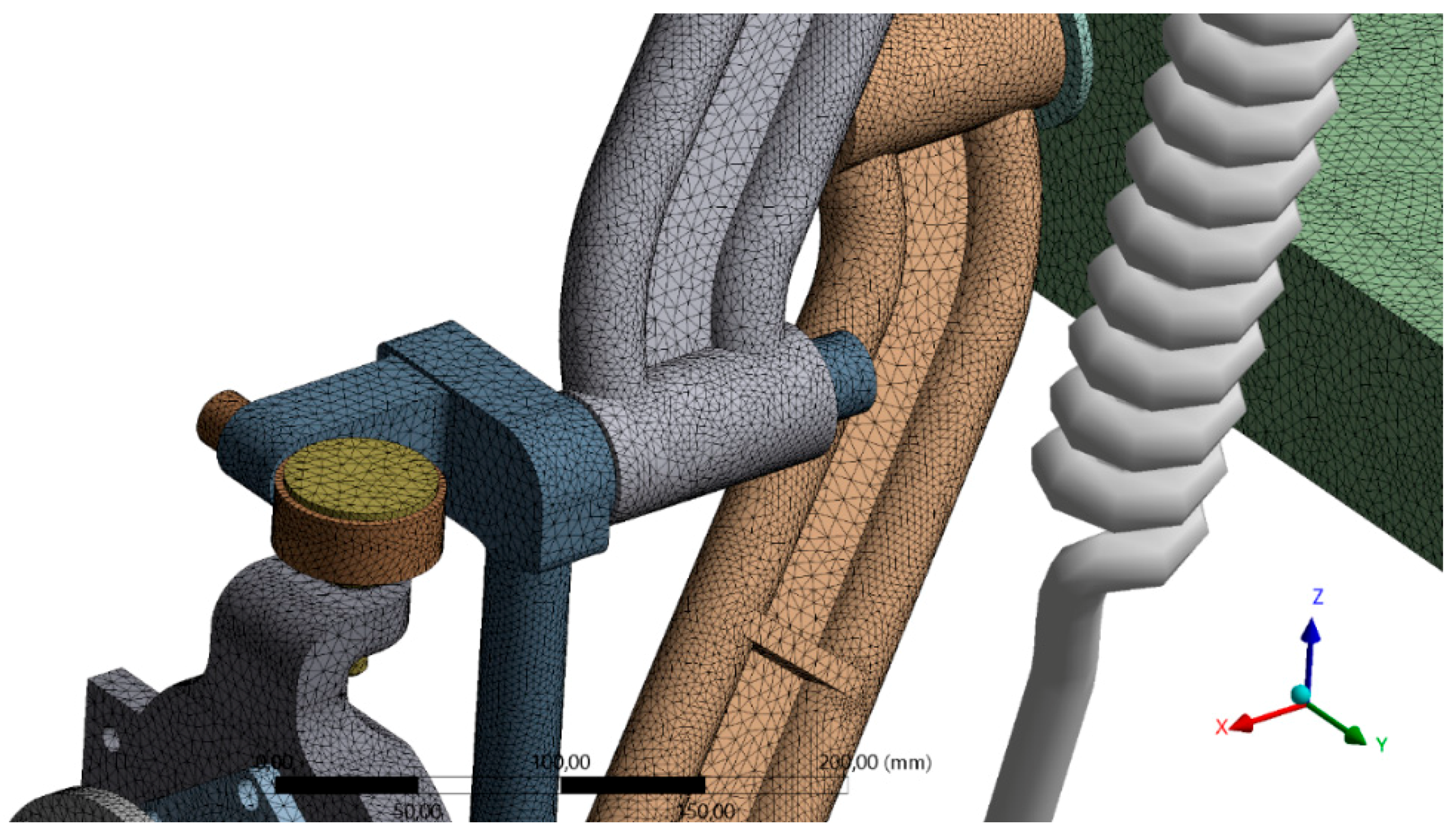
All strength analyses were carried out by the Ansys 2019R3 programme (Ansys Inc., Canonsburg, PA, USA). This software belongs to most widely used software for performing static or transient analyses of mechanical components by means of the finite element method (FEM) [27,28]. The accurate geometry of the designed 3D components was imported from the programme Catia V5R20 (Dassault Systèmes, Paris, France). Subsequently the authors analysed the stresses for individual driving regimes. First of all, we realised the finite element analysis for driving in the curves. The linear tetrahedron elements were used for meshing the models. Details of FEM mesh is shown in Figure 13. The force edge conditions (load) were defined in the previous part. The loading forces were calculated for the tyre adhesion limit with the road. Therefore, the calculation includes the maximal loads of the considered driving regimes. The edge conditions that model the attachments correspond with the described real state.

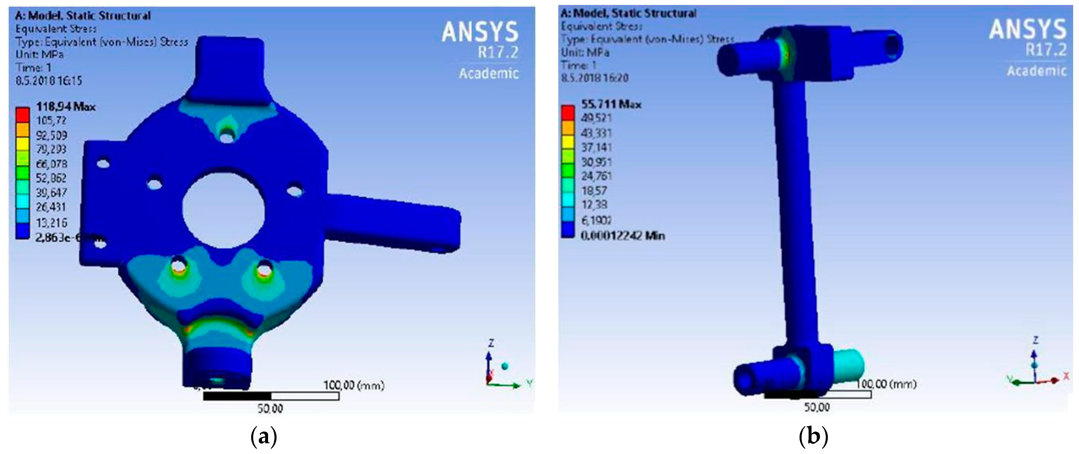
Based on simulation we detected that the largest stress of 118.9 MPa is on the wheel pivot bolt (Figure 14a) and is placed in the bottom part close to the attachment of the bottom knuckle bolt (there is also the largest force during driving in the curve R_B = 3590.0 N). However, it is a safe stress because the pivot bolt material achieves the yield strength up to R_e = 590 MPa.

In the case of the vertical control arm the stress is 55.7 MPa (Figure 14b) and it does not present any big danger from the point of view of the load carrying capacity.

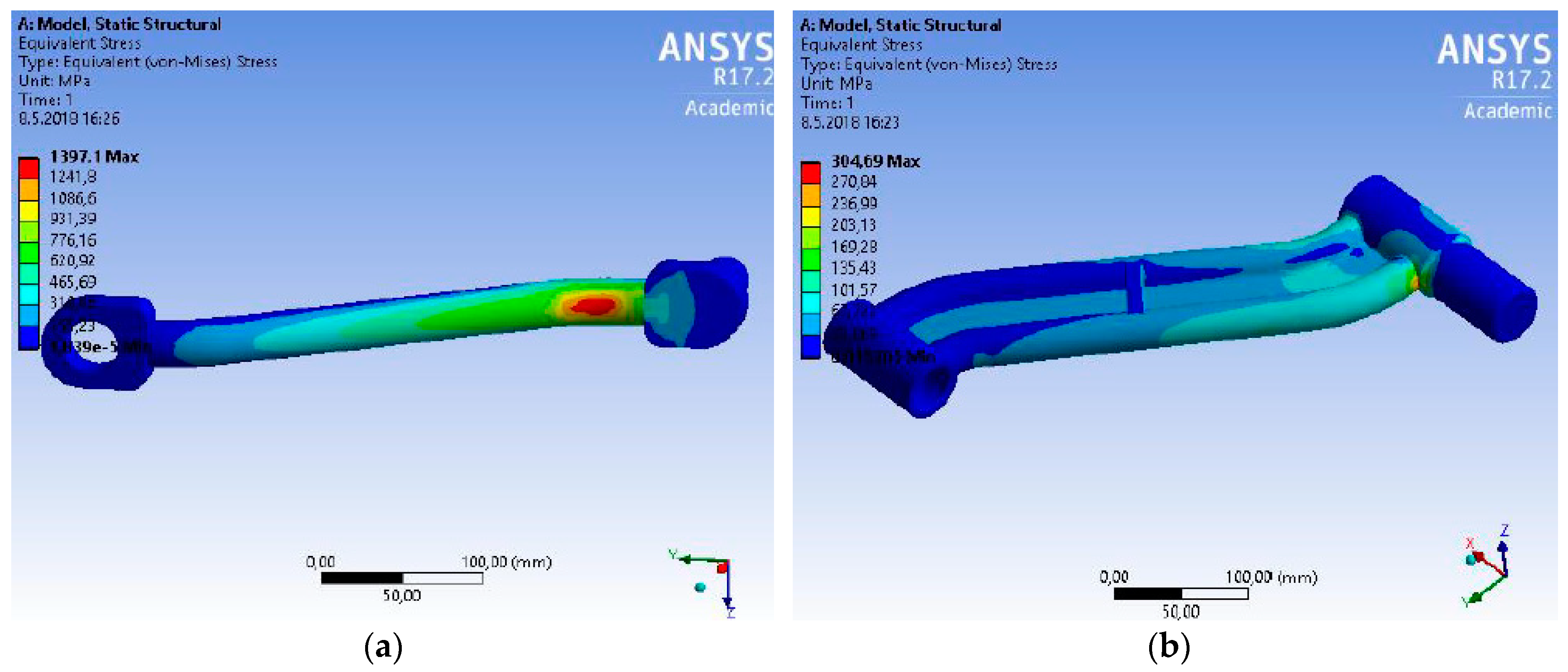
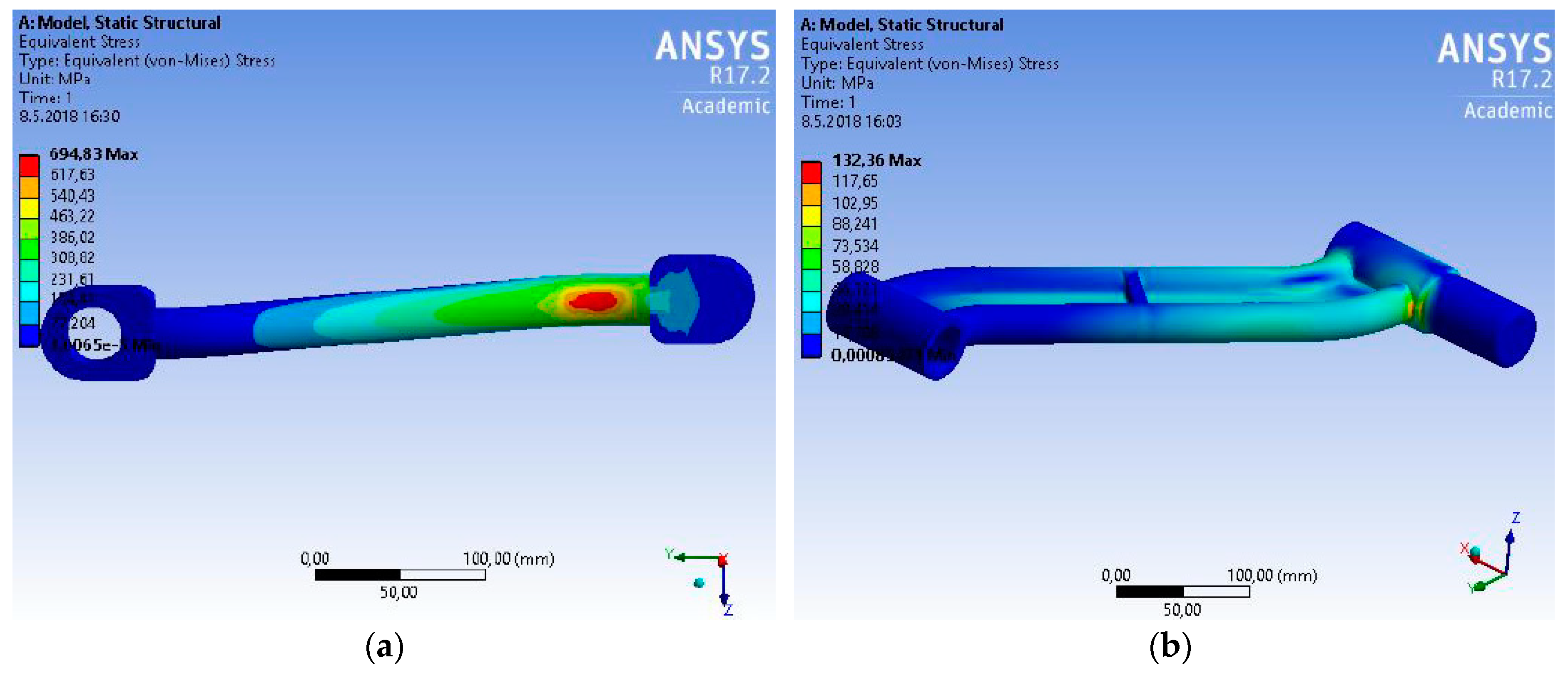
The material of the vertical control arm—25CrMo4—achieves the yield strength of R_e = 760 MPa [29]. The highest stress can be found in the point where the vertical control arm is attached in the control arm. However, the biggest force performs in the bottom part of the control arm. The fact that the largest stress is not present is caused due to attaching the knuckle bolt—this attachment together with the attachment of the control arm is in one plane. In this way the force is transferred directly to the upper control arm by pressure. In the case of the bottom control arm the situation is more complicated. The original control arm from the design (the utility model) is created from one pipe only. The component designed like this would not withstand because the maximal achieved stress is 1397.0 MPa. The designed component is placed close to the attachment base into the frame. This control arm consists of one pipe only. The design of the control arm is more sophisticated. If we compare the original (Figure 15a) and the new design (Figure 15b), a change is visible. The highest stress is not in the carrying pipe any more. It is moved into the base of the control arm attachment with the frame. The adapted control arm achieves the maximal stress of 304.69 MPa. This is again an acceptable value, if the yield strength is R_e = 590 MPa. The deformation of the control arm end at the maximal load is 1.3 mm.

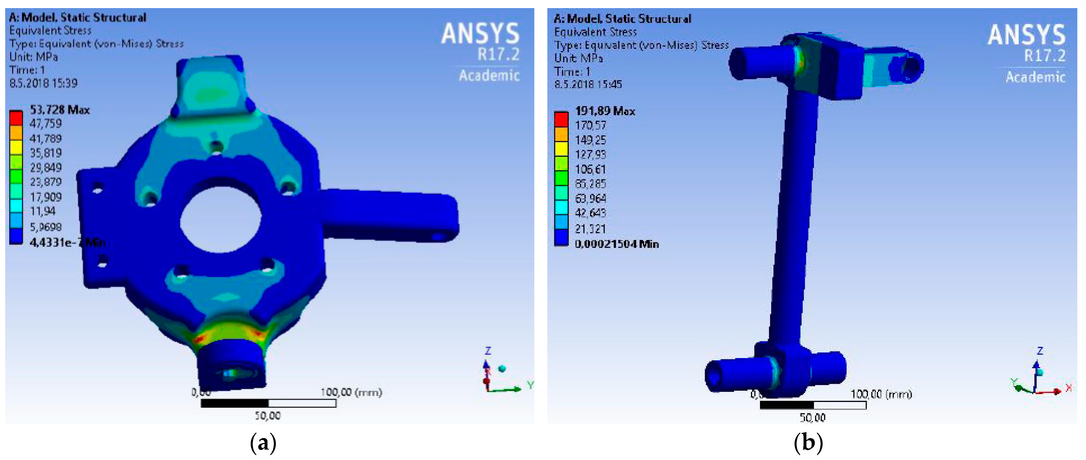
The adaptations concerning the control arm consisted in increasing the pivot diameter. Originally a pivot for attaching into the frame with the diameter of 30 mm was used. The new design has the diameter of 48 mm. This step reduced the maximal stress by approximately 80 MPa. The bore for the pivot-pin bush for attaching the vertical control arm was also adapted from the value of 30 mm to the current 95 mm. This step reduced the maximal deformation. There was no need to analyse the upper control arm. It is due to a lower load compared with the bottom control arm. Due to the braking process the largest stress was on the wheel pivot bolt close to the point of attaching the bottom knuckle bolt (Figure 16a). This stress (53.728 MPa) is acceptable because the yield strength of the pivot bolt material is R_e = 590 MPa.

The highest stress (due to the braking process) on the vertical control arm can be found in the attachment of the upper control arm. It is probably caused by the fact that the attachment of the upper knuckle bolt and the upper control arm are not in the same plane. The equivalent stress achieved the maximal value of 191.89 MPa (Figure 16b). It is a safe value because the yield strength of the vertical control arm material (steel 25CrMo4) is R_e = 760 MPa.

During the analysis of the brake load on the control arms we can compare the original (Figure 17a) and adapted model (Figure 17b). The original model would probably withstand the load detected; however, the safety due to the ultimate state would be of a threshold character. At the same time the model showed a relatively big deformation, approximately 13 mm. The maximal stress is in the same point as during passing a curve. The adapted control arm showed a very small deformation, less than 1 mm. The maximal stress was detected in the area of attaching into the vehicle frame. It achieved a value of 132.36 MPa and it can be considered a safe value from the point of view of the material yield strength—R_e = 760 MPa.

The eigenmode analysis and the analysis of the oscillation frequency, i.e., the modal analysis, provides the primary information concerning the verification and correctness check of the model setup for the axle investigated and its dynamic properties [30,31]. We carried out the modal analysis on a model where damping was not defined. Then the calculation proceeds as follows:

$$\mathit{M}·\ddot{\mathit{q}}+\mathit{K}·\mathit{q}=\mathbf{0},$$

(53)

where M is the mass matrix, K is the stiffness matrix and q and $\ddot{\mathit{q}}$ are position and velocity vectors, respectively.

The solution of the system equations of motion (53) we are searching in the following form:

$$\mathit{q}\left(t\right)=\mathit{y}·\sin \left({\mathsf{\Omega }}_0·t\right),$$

(54)

where Ω₀ is the angular eigenfrequency of the system, y is the vector of the amplitudes of the eigenshape oscillation of the system.

Through the well-known procedure we will obtain a spectral matrix of the eigenvalues of the system:

$${\mathsf{\Omega }}^2=\left[\begin{array}{cccccc}{\mathsf{\Omega }}_1^2& 0& .& .& .& 0\\ 0& {\mathsf{\Omega }}_2^2& .& .& .& 0\\ .& .& .& .& .& .\\ .& .& .& .& .& .\\ .& .& .& .& .& .\\ 0& 0& .& .& .& {\mathsf{\Omega }}_n^2\end{array}\right],$$

(55)

whose square roots are the angular eigenfrequencies of the axle oscillation Ω (rad·s⁻¹), or a small adaptation of the eigenfrequencies of the axle oscillation f (Hz).

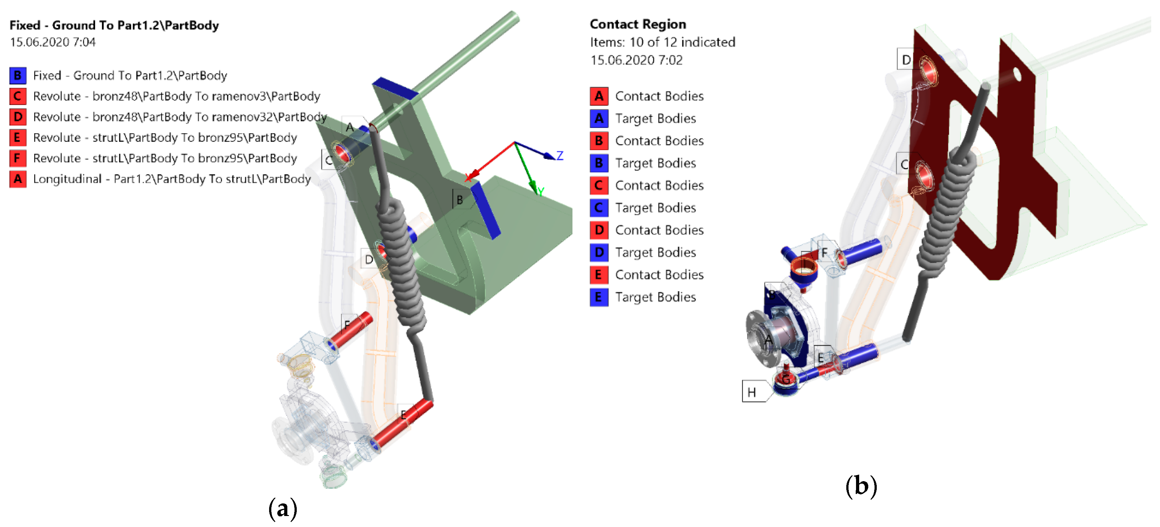
After performing the static FEM analyses the authors continued with the modal analysis of the wheel suspension. At first it was necessary to define the links (Figure 18a) and the contact surfaces of the design (Figure 18b). Of course, there was an effort to converge towards the real state. The links used in Figure 18a describes the kinematic couples used in a real wheel suspension of a car. The spring loading element is replaced by a spring link. It was assigned the stiffness of 10 N·mm⁻¹. This link will be assigned the necessary damping during the dynamic simulation. No damping was considered or the modal analysis.

The system damping was not assigned as the input for the given simulation of this element. The boundary conditions for the modal analysis were defined by taking all degrees of freedom away. They were taken away from the frame body. They were realised through the link of type “fixed body to ground” on defined surfaces. The first six eigenfrequencies and shapes of the wheel suspension were investigated.

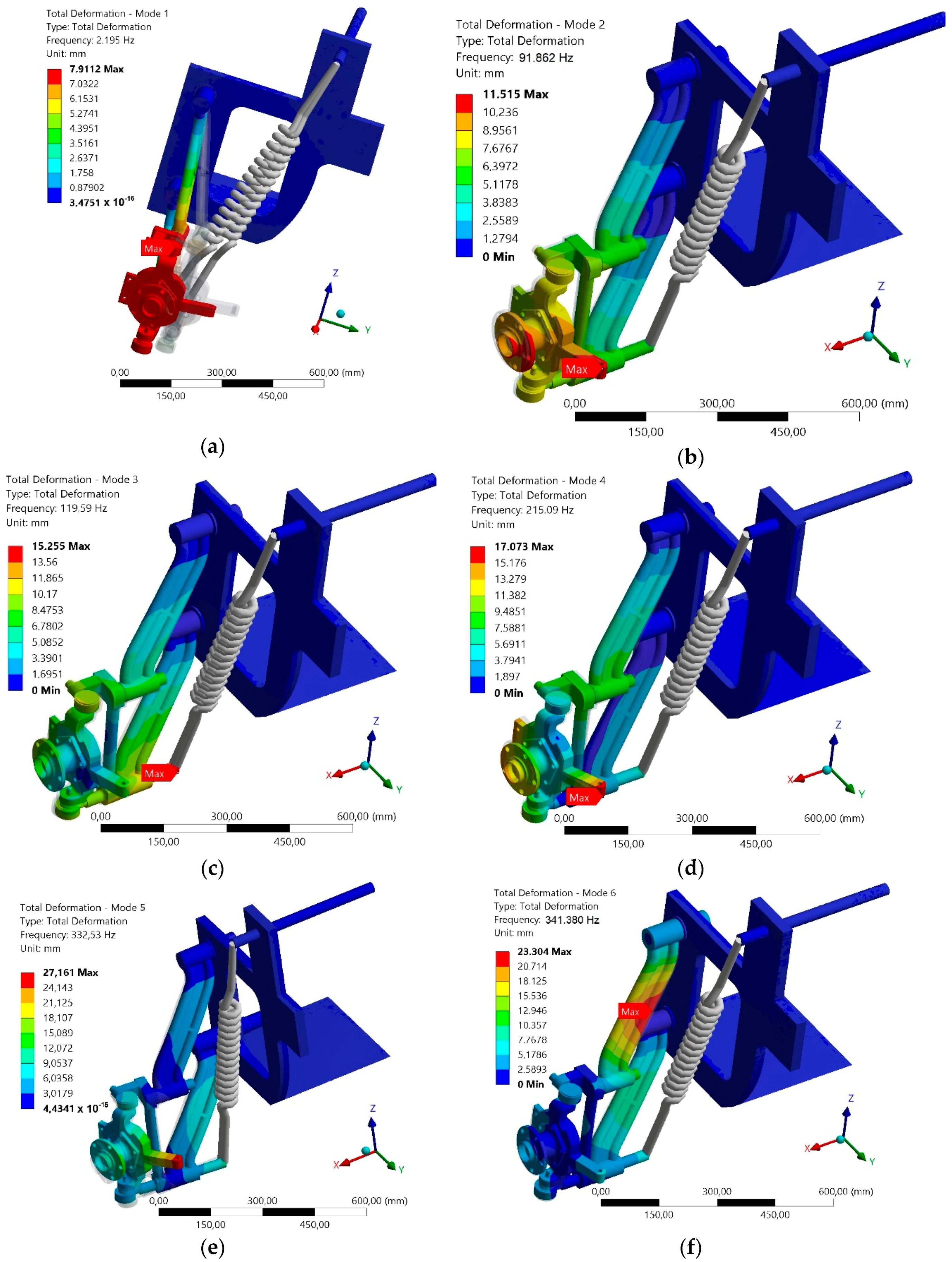
Figure 19 depict the first six eigenmodes of the undamped oscillation of the half-model of the investigated axle acquired by calculations from the Ansys programme. As it is an independent wheel suspension, it was sufficient to carry out a modal analysis of only a half-model of the axle. The values of the eigenfrequencies shown in

Table 3. The eigenfrequencies of the axle half-model oscillation, undamped oscillation.

	Angular Eigenfrequency		Eigenfrequency
Eigenmode	Designation	Value (rad∙s−1)	Designation	Value (Hz)
1st	Ω1	13.758	f1	2.195
2nd	Ω2	576.893	f2	91.862
3rd	Ω3	751.025	f3	119.590
4th	Ω4	1350.765	f4	215.090
5th	Ω5	2088.288	f5	332.530
6th	Ω6	2143.866	f6	341.380

correspond with these shapes. However, in reality there will always be certain damping and therefore the eigenfrequencies of oscillation will achieve a little bit lower values.

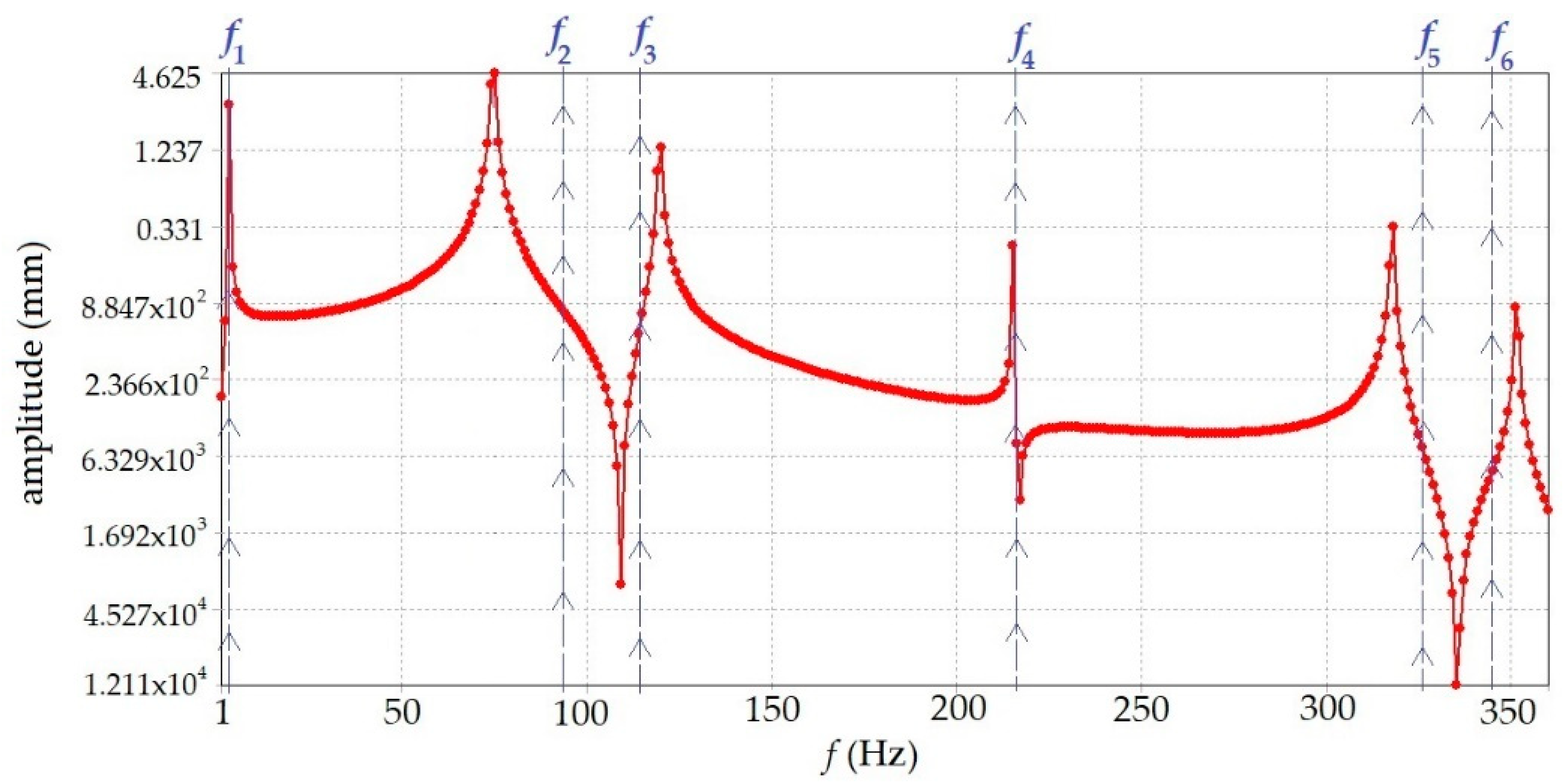
They correspond with the detected eigen-frequencies. As the authors expected the first eigenmodes (Figure 19a) corresponds with the working oscillation of the suspension. In the second up to the fourth eigemodes (Figure 19b–d) we can see the system oscillation. The oscillation develops in the direction of the lowest stiffness of the system at higher excitation frequencies. The elimination or a shift of the eigenmodes to a higher excitation frequency can be achieved by increasing the suspension control arm stiffness. The frequency analysis of the axle model was also realised (Figure 20).

Figure 20 depicts an amplitude and frequency characteristic of oscillation. It is also acquired from the Ansys programme for the axle half-model.

The largest oscillation deviations are indicated in the area of the eigenfrequencies. As already mentioned, damping of the system was not defined for the modal analysis and therefore the amplitudes achieve also negative values. In the case of defining the system damping they would be depicted only in the positive part of the amplitude and frequency characteristic.

6. Sensitivity Analysis of the Vehicle

The programme Motionview was used for realising the sensitivity analysis. The programme Motionview from the company Altair (Altair Engineering, Inc., Troy, MI, USA) is complex simulation software. It serves for the multi-body (MBS) dynamic simulations. The results of the vehicle simulations are depicted in the form of animations and diagrams. The vehicle model is defined parametrically in a coordinate system x, y, z. It is defined by points (Figure 21a) that represent the individual ball joints and rubber arrangements of the control arms, stabilisers, dampers, etc. The capability of the programme to model parametrically enables the users to create the models in an automated way. This gives extensive possibilities of the parametric studies, e.g., determining the influence of the kinematic parameters of the axle on the dynamic response of the vehicle. The programme is able to simulate the whole vehicle including the engine, gearbox, steering, wheels, brakes, the front and rear axle. It enables to select the engine arrangement and also the options of a driven axle or axles. These parts of the vehicle create systems in the programme that can be parametrically adapted. The post-processing programme Hyperview serves for depicting the simulation results of the programme Motorview. It visualises the simulated car in various situations. They can be—e.g., accelerations, braking, passing a curve, slalom, etc. The results of the analysis can be depicted graphically. The followed values can be presented in dependence on time, speed, path or another quantity determined by the user. The diagrams are synchronised with the video of the car’s operation. Then it is possible to follow the quantity values in time and the vehicle’s dynamic behaviour.

At first it was necessary to determine the space position of individual axle elements (i.e., all ball joints, silent-blocks, damper positions, springs, etc.). Due to the symmetry of the axle model, the measurement of only one side of the vehicle was sufficient. The car measurements were carried out at the loaded state by its weight (i.e., at the simulated loading obtained from the FEM analysis). The centre of the wheel bearing was taken as the reference point. From this point, the individual axle elements were measured. The individual points were measured by a measuring tape, calliper, bubble-level and angle iron with an overall accuracy of ± 5 mm. The programme created the vehicle model.

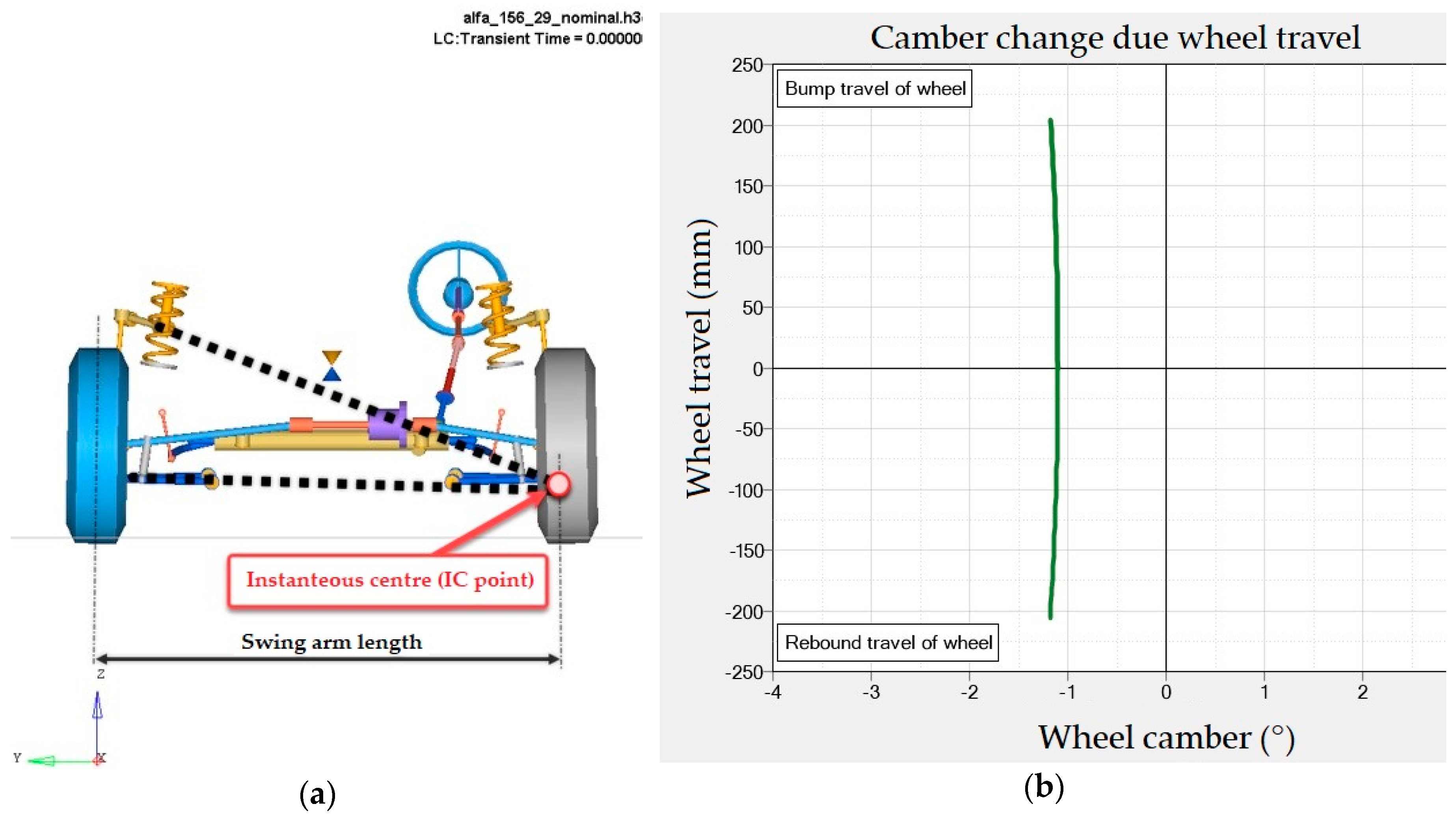
At first the authors were dealing with characterising the change of the wheel deviation in the case of parallel springing the axle. This occurs during the vertical motion of the front axle of the simulated car. Figure 21b shows the created characteristic of the change of the wheel deviation.

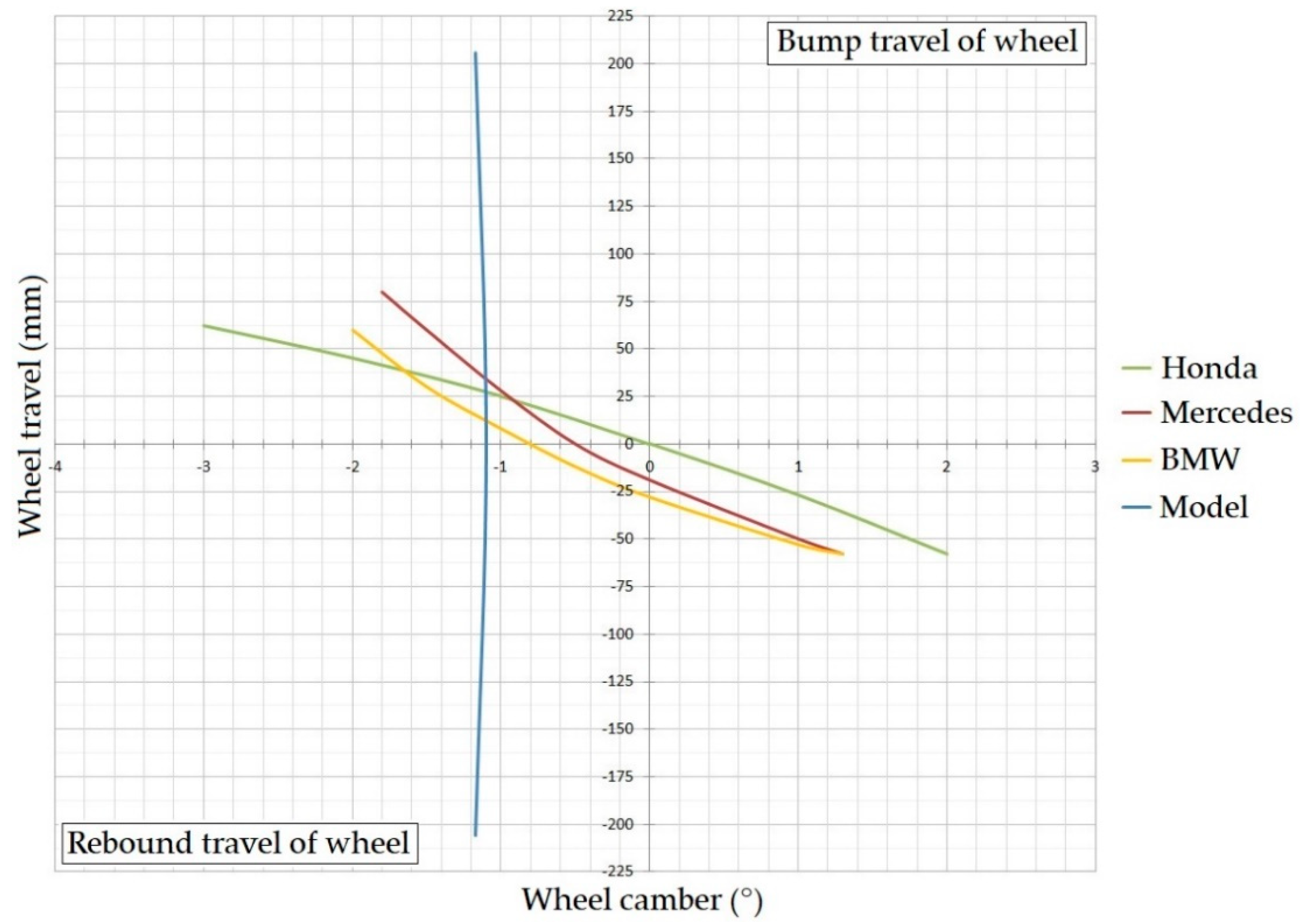
The characteristic in Figure 21b shows that the wheel deviation is almost constant in dependence on the spring compression and the weight transfer of the axle. It is caused by the fact that the control arms practically do not change the angle of the mutual angular rotation during a vertical motion. The authors assessed the influence of their technical solution has similar effects as adjusting the geometry in the case of the off-road racing vehicles, e. g. the racing car Ford Shelby Baja Raptor. This vehicle has an axle with parallerly long control arms. This design (of course, a more expensive one) in the case of the spring compression and spring loading has a constant characteristic of the wheel deviation. The authors compare their findings with the characteristics of the car BMW, Mercedes-Benz (class E) and Honda Accord. Professor Reimpell at al. described these vehicles in his book [32]. The graphical dependences depict the behaviour of the front axle of these car brands in the case of the spring compression and spring loading of the axles. The diagram (Figure 22) includes also the characteristic of the simulated car of the authors.

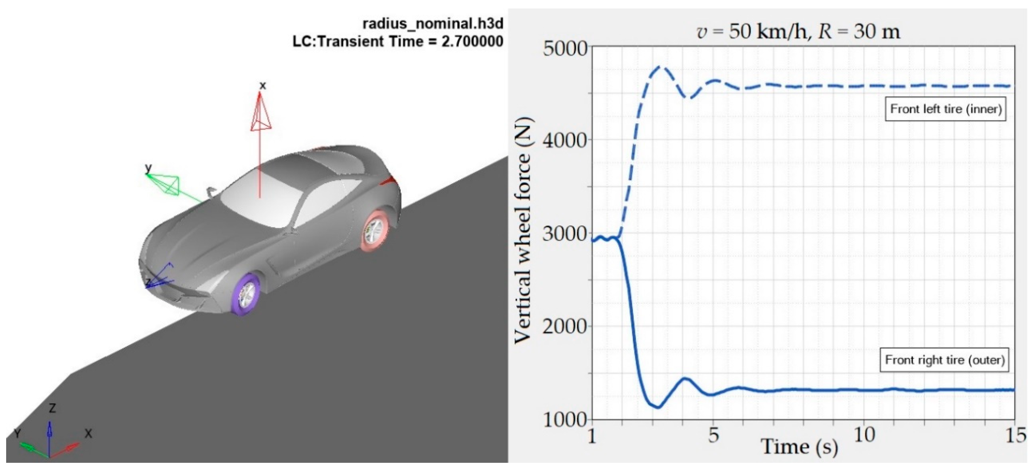
The Motionview programme simulated a pass of the vehicle through a left-hand curve with a radius of R = 30 m at the car speed of v = 50 km·h⁻¹. Before cornering the car drove straightforward 30 metres due to the numerical stabilisation of the initial conditions. The simulation itself took approximately 20 s. The task of the simulation was to follow the forces performing on the front wheels. The values of the simulated forces will serve for verifying the input data of the analytical and dimensional calculation. The diagram of the performing forces is depicted in Figure 23. The external wheel had almost a perpendicular contact with the road thanks to a zero deviation of the wheel—see the previous diagram. The smaller this force is, the stronger tendency of the car to come out of the turn is—the so called understeering.

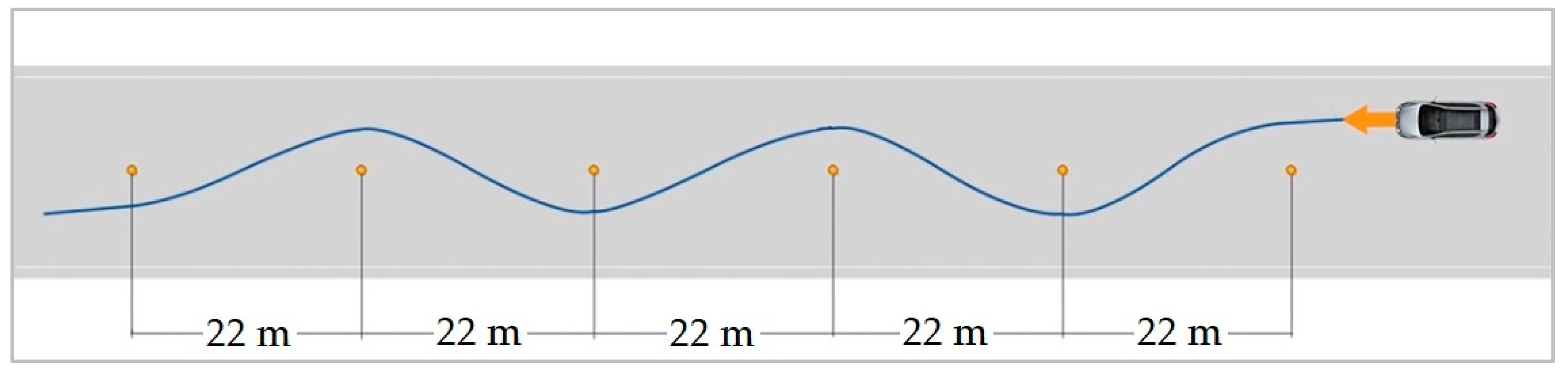
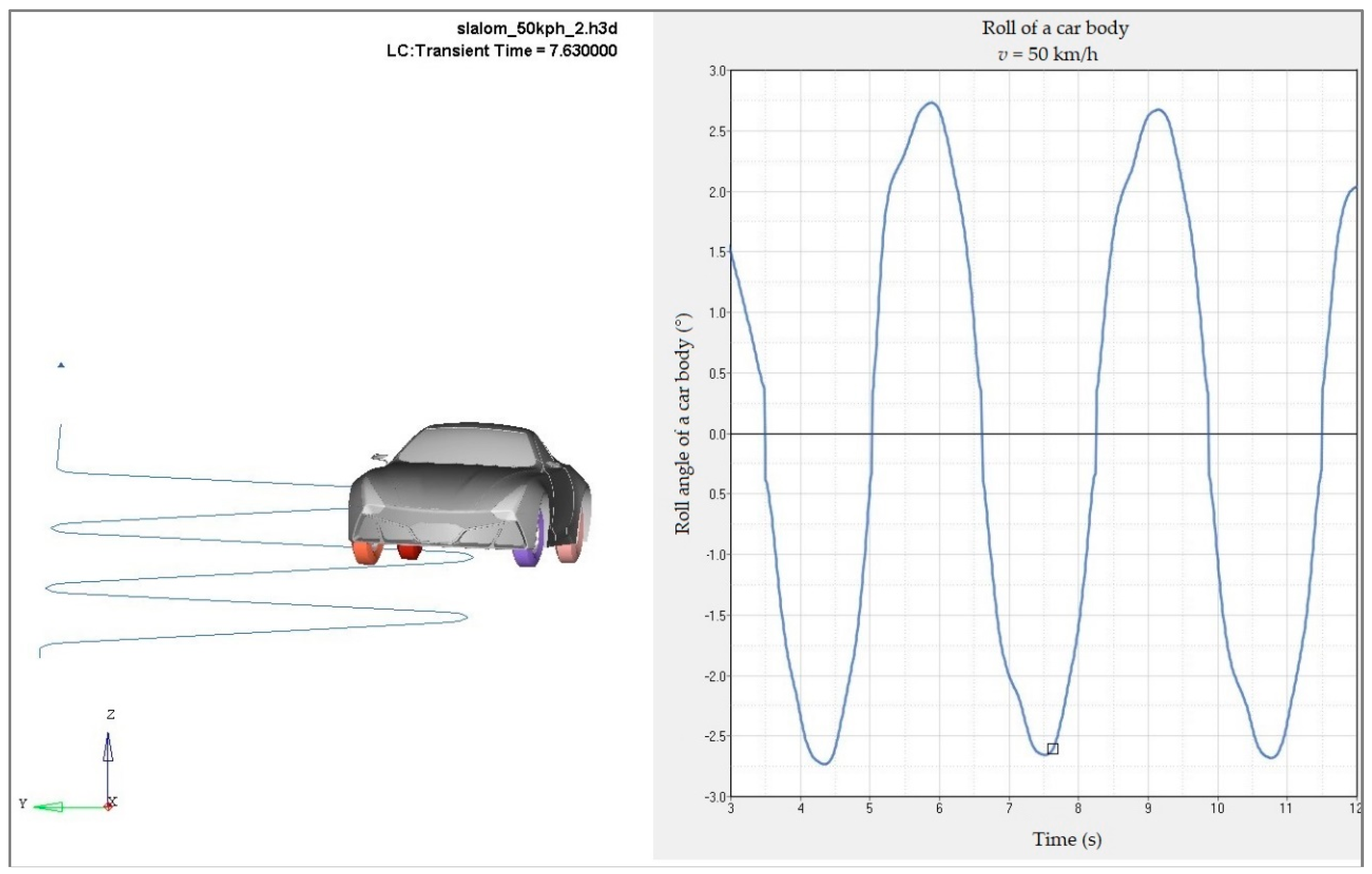
The authors then carried out an analysis of the car’s slalom. The goal of the slalom will be the observation and comparison of the car’s roll during driving between cones at the speed of 50 km·h⁻¹. The real pass of the car with the Motionview simulation will be compared. The simulated pass was based on a standardised test (Figure 24). Results of the car’s bodywork roll angle analysis are shown in Figure 25.

A text file had to be created for making the simulation procedure. The file contained the vehicle trajectory through the space coordinates. This corresponded with the real pass best. After entering all necessary parameters, the programme calculated the simulation which enables the observation the output—the bodywork roll. The simulation is shown in Figure 26. The angle of roll of the car’s bodywork was approximately 2.5°. This value seems comparable with the conventional vehicles.

In the next steps the authors will carry out experimental measurements on their own testing vehicle they made by themselves. Until now all analyses have confirmed the correctness of the design. The simulations were important conditions for verifying the safety of the design. The dynamic analysis of the vehicle is the last analysis realised before the test drive.

7. Dynamic Analysis of the Vehicle in the Programme Simpack

The computer programmes for creating the MBS models of the vehicles and simulation of their dynamic properties have an irreplaceable place and their utilisation for developing the cars is an absolute necessity. The simulation of the vehicles is used especially for improving the quality and safety of driving and driving properties of the cars on the basis of the target requirements.

This section is aimed at describing the vehicle as a MBS system and for assessing the simulation results created in the Simpack programme (Dassault Systèmes, Paris, France). The MBS Simpack programme enables creating and simulating the mechanical systems from the simpler car sub-systems up to the complicated non-linear mechanical systems of whole vehicles. The models can be created in the 2D interface in the form of block schemes similar to the program Matlab [33,34] or more often in the 3D interface of the programme. The user can observe a three-dimensional model of the mechanical system created. The visualisation of the motion, acting forces as well as other followed parameters is possible [35,36,37].

The computer model of the mechanical system is created by rigid bodies that are connected by the force elements, then by the mechanical and kinematic joints. As the MBS model of the vehicle contains also the kinematic joints the mathematical model of the car is created by the differential and algebraic equations in the following form:

$$\left[\begin{array}{cc}\mathit{M}& {\mathit{D}}^T\\ \mathit{D}& \mathbf{0}\end{array}\right]·\left[\begin{array}{c}\mathit{q}\\ \mathit{\Lambda }\end{array}\right]=\left[\begin{array}{c}\mathit{F}\\ \mathit{\gamma }\end{array}\right],$$

(56)

where M is the mass matrix, D is the Jacobian matrix, q is the vector of generalised coordinates, Λ is the vector of Lagrange multipliers and F is the load vector of the system (kinematic excitation, performance of the external forces, etc.) and $\mathit{\gamma }=\mathit{D}·\ddot{\mathit{q}}$ [38,39,40].

The MBS dynamic analysis of the vehicle system requires defining the initial conditions. In this case it is the definition of the initial speed, i.e., the velocity vector. Based on this information, the created equations of motion (56) are solved.

The importance of the MBS simulations of the investigated vehicle consists in the simplicity of changing a certain parameter and the subsequent analysis of this change. Although the results of the simulation calculations never fully correspond with the reality, they are sufficiently accurate for us to gain an overview about the properties of the tested car.

The model parameters of the tested vehicle defined in the Simpack programme are based on the data from Table 1. For the model of the investigated vehicle to represent the real vehicle´s behaviour as realistically as possible, the following requirements were fulfilled during creating its MBS model:

• The required model kinematics as a whole including the kinematic sub-systems—aimed at the tested front axle.
• The spring loading system of individual wheels.
• The representation of the link elements of the model.
• They dynamic forces in the tyres.
• The model must not be too complicated; the time of the calculation has to remain acceptable.

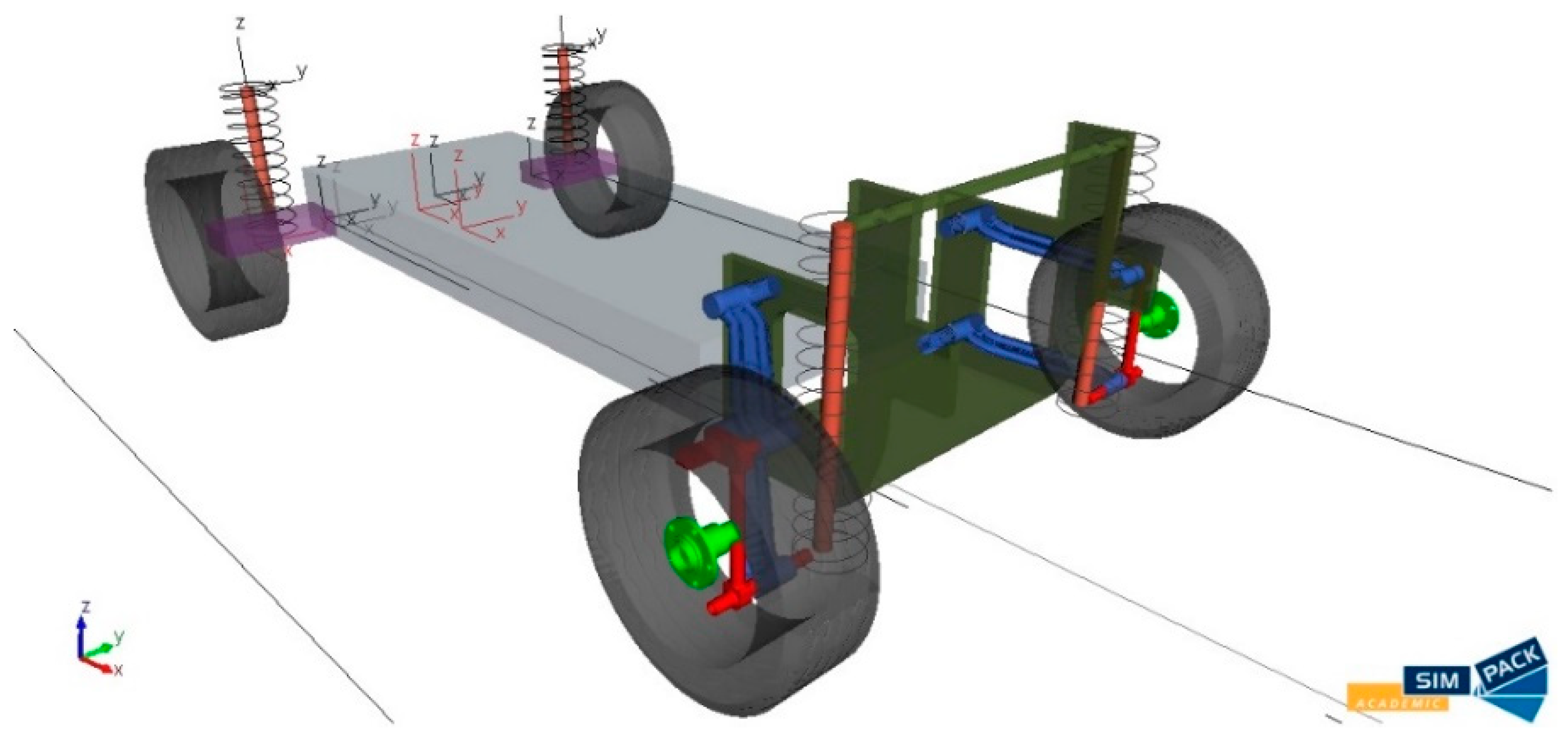
A coordinate system was defined for creating the MBS model. The individual bodies have a defined weight, moments of inertia and positions of the CoG.

Figure 26 depicts the MBS model of the analysed vehicle created in the Simpack programme.

The next step of creating a full MBS model of the vehicle is to define the road parameters. It means especially defining the length of a direct section, parts of the curves, their parameters and number, the method for determining the contact of the tyre with the road, the layout of the road irregularities, etc.

During the simulation of driving the car with the tested front axle the following driving analyses were carried out:

• In the curve with defined parameters (Figure 27).
• On a straight path with irregularities for assessing the oscillation properties of the car.

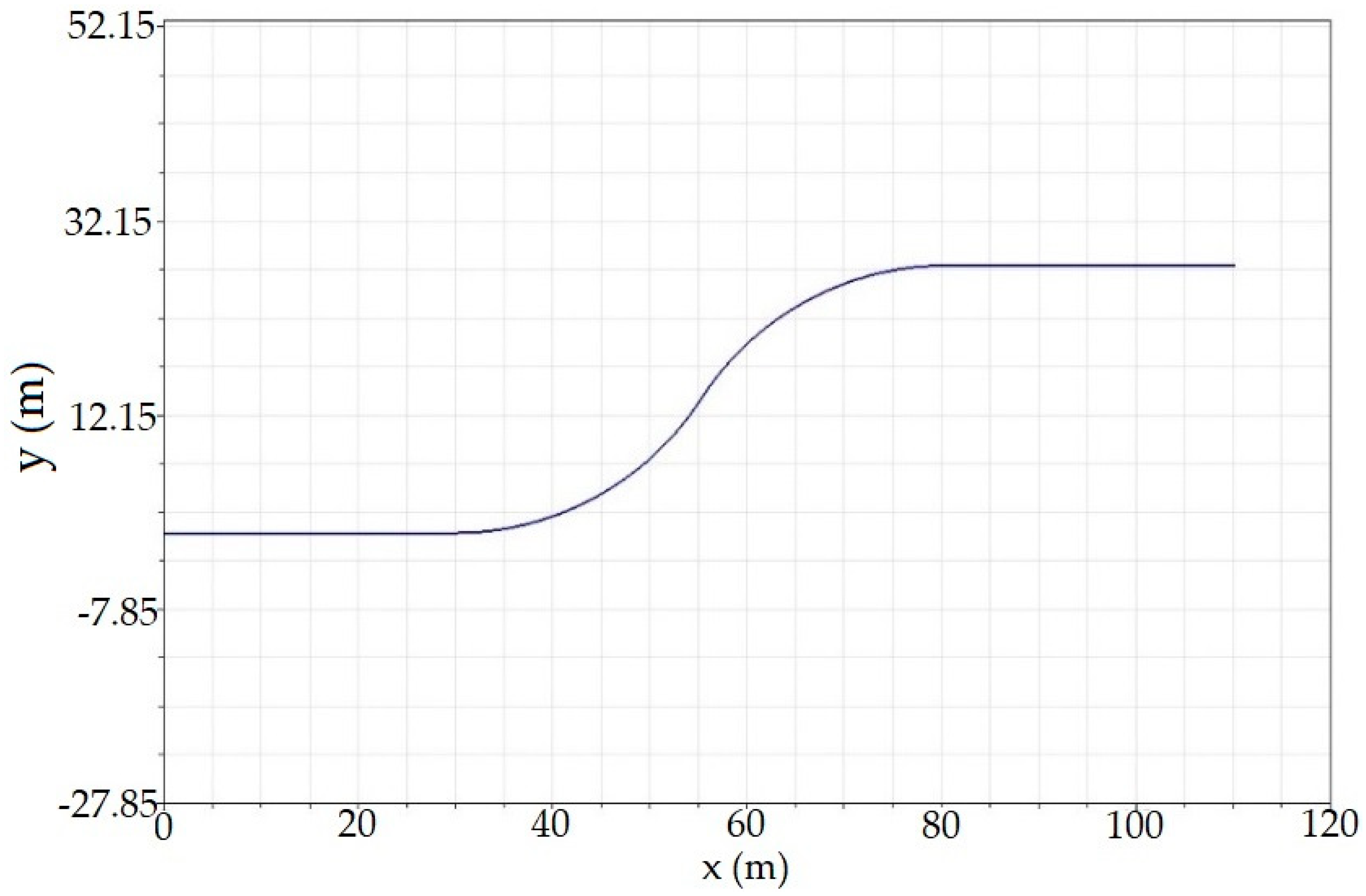
The road model was created in the programme Simpack through defining the necessary data. A simple road profile with curves with the radius R = 30 m was used for simulating the drive in a curve. The road layout is shown in Figure 27.

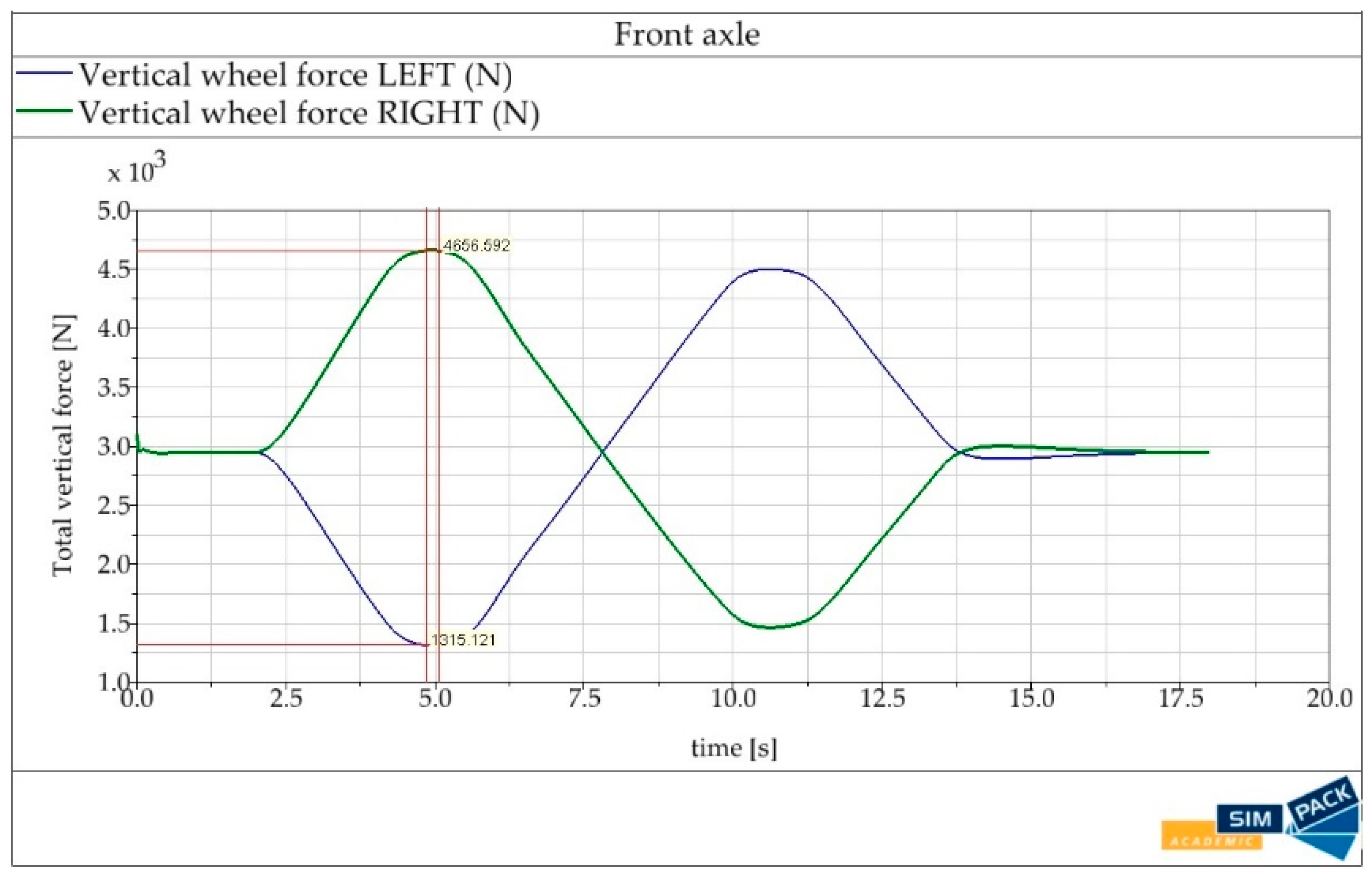
Figure 28 shows the course of the vertical wheel forces of the front axle tested. The CoG of the car is considered in the longitudinal vehicle axis, i.e., in the middle of the wheel spacing. As we can see the vertical wheel force in the straight part of the path corresponds with the vertical car load and was stabilised on the value of approximately 2945 N for both wheels.

However, if the vehicle enters a curve, a change of the load distribution on individual wheels develops due to the performance of the centrifugal forces. In our case the car enters a right-hand bend at first. Therefore, the wheel force value on the external wheel increases (the green curved line) and its maximal force for the given driving conditions (v = 50 km·h⁻¹; R = 30 m) is 4656.592 N. On the contrary, the internal wheel (the blue curved line) is relieved and its minimal value in the followed section is 1315.121 N. The calculated values show that driving a car with the tested axle will be safe at the speed of 50 km·h⁻¹ and the curve radius 30 m. The internal wheel is still able to transfer sufficient large driving, braking and lateral forces.

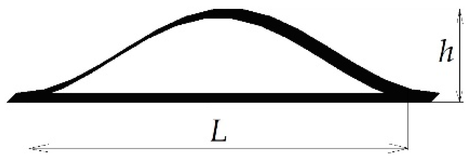
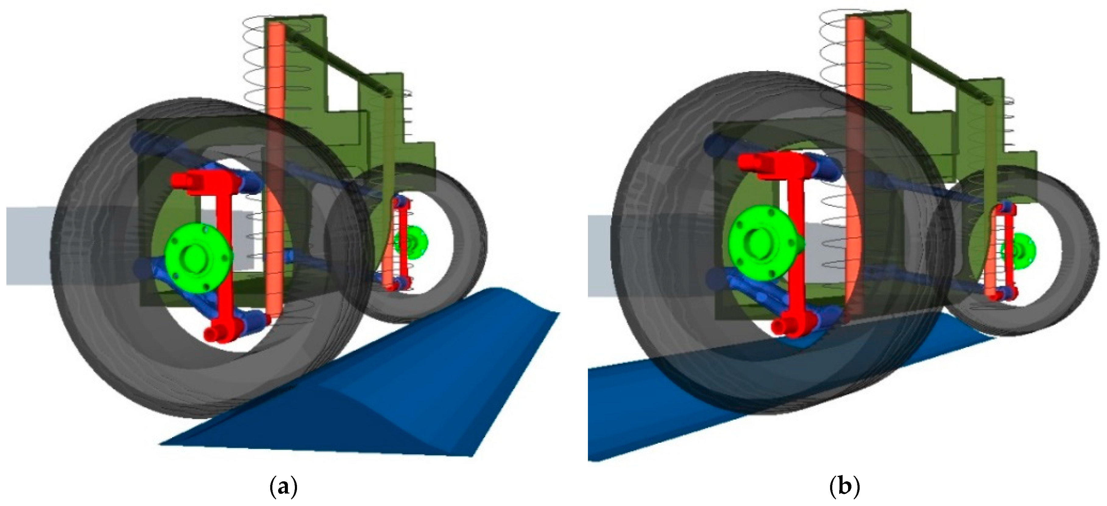
Then we observed the operation of the wheel forces on the front axle of the tested vehicle during driving over an obstacle. The obstacle geometry is depicted in Figure 29. It was a simple obstacle under both wheels (Figure 30).

We defined two heights of the obstacle h and the length of the obstacle L was the same for both cases:

• The first case: L = 0.5 m; h = 0.025 m.
• The second case: L = 0.5 m; h = 0.100 m.

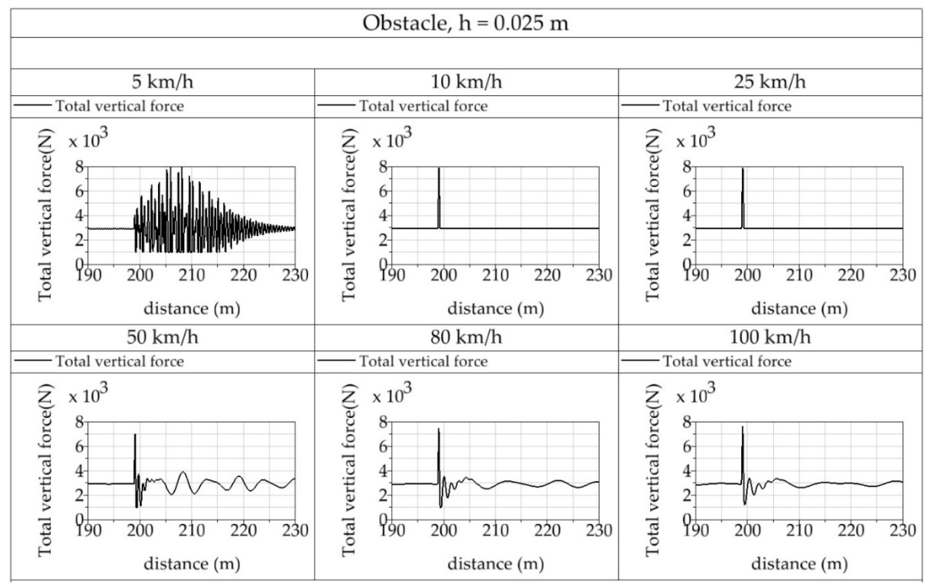
The simulation calculations of driving over obstacles were realised for a larger range of speeds and we chose only a few of them for the presentation, particularly the following speeds: v = 5 km·h⁻¹; v = 10 km·h⁻¹; v = 25 km·h⁻¹; v = 50 km·h⁻¹; v = 80 km·h⁻¹ and v = 100 km·h⁻¹.

Figure 31 and Figure 32 depict the graphical outputs. For a better comparison the operations are depicted in dependence on the passed path (the horizontal axis).

These diagrams depict the operations of the vertical wheel forces of the right wheel of the front axle. The vehicle was overcoming the same obstacle with the whole front axle at the same time. This corresponds with the situation of driving over a retarder. Therefore, it is sufficient to show the results only for one side of the vehicle, i.e., for one wheel.

Figure 31 shows the operations of the observed quantities. It is a case of overcoming an obstacle with the height of h = 0.02 m. We can see the car was excited by this unevenness at the moment of overcoming and the vertical wheel force increased. In the situation with v = 10 km·h⁻¹ and v = 20 km·h⁻¹ the maximal wheel force at the moment of the run up is the same. The higher speeds, i.e., v = 50 km·h⁻¹, v = 80 km·h⁻¹ and v = 100 km·h⁻¹ at which the car overcomes this obstacle cause a situation when the vehicle oscillation fades out more strongly behind the obstacle. It is caused by the inertia of motion of the vehicle parts in the front axle and gradual damping the oscillation. The instantaneous maximal values of the dynamic force at the moment of overcoming the obstacle (unevenness) do not represent any significant ganger from the point of view of safe driving. The most interesting case seems to be the operation of the vertical force at the speed of v = 5 km·h⁻¹. In spite of a relatively low speed the system is oscillated most significantly just at this speed. The situation can be caused by combining the given driving speed, the amplitude and wave length of the unevenness. This excites the oscillation of the front part of the vehicle. Our optimisation will be aimed at achieving suitable oscillating properties together with the aforementioned driving conditions.

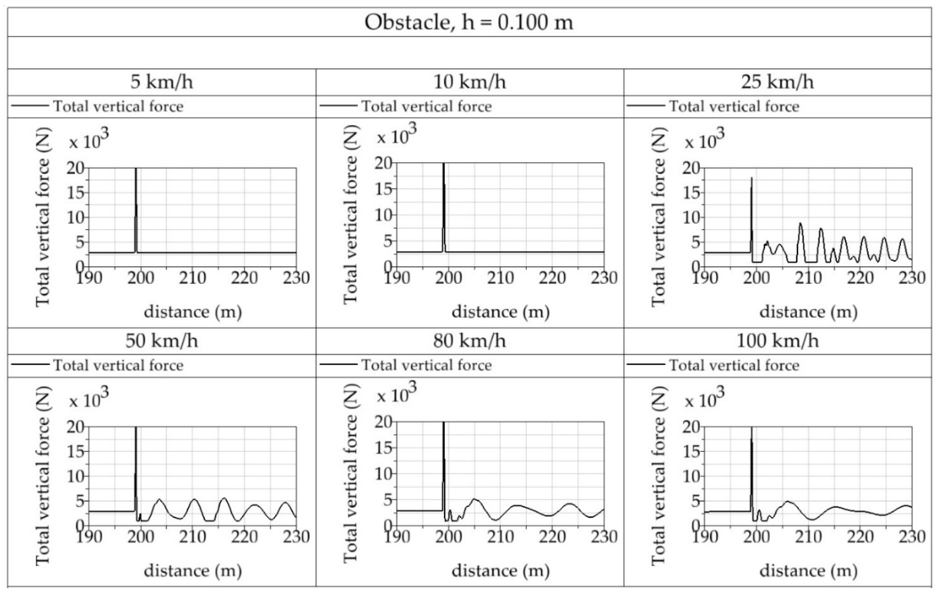
When the car overcomes an unevenness with the height of h = 0.100 m, the situation is different (Figure 32). If the vehicle is overcoming the given obstacle with a low speed (v = 5 km·h⁻¹), the operation of the vertical wheel force is not that strong. The force is then characteristic only by its current growth of its value during running up the obstacle. The simulation result for the speed on 10 km·h⁻¹ has a similar character. When the car drives at the speed of v = 25 km·h⁻¹, v = 50 km·h⁻¹, v = 80 km·h⁻¹ and v = 100 km·h⁻¹ a typical oscillation of the vehicle front part develops and it is typical that it fades out gradually. Similarly, as in the previous case the instantaneous values of the vertical wheel forces in the observed driving movements do not lead to any serious threat of the driving safety.

The results presented in Figure 31 and Figure 32 are valid for driving in a straight direction. Let us take into account the influence of the inertial forces on the values of the vertical wheel forces during passing a curve (Figure 28). We can assume that is this case a situation threatening the driving safety could develop—especially due to the vertical force of the internal wheel in contact with the road.

The extent of the dynamic analyses of the vehicle with the designed axle is currently in this research phase limited on the primary tests aimed at detecting the fundamental properties of the given mechanical system of the car. The currently achieved results are also presented in this scope. The vehicle mechanical system represents a complicated unit. This system is to be investigated thoroughly—e.g., analysing the vehicle during driving on a road with unevenness defined by the performance spectral density or directly measured unevenness. The next aim of the vehicle project is to implement the already modelled flexible bodies into the dynamic model of the car. In this way it is possible to observe the distribution of the stresses and deformations of the key components under the dynamic load. The value added of the given research is that it will be realised directly on the road. It will be possible to verify the driving properties of the vehicle on a functional prototype (Figure 6) by experimental tests. From the point of view of the crew’s safety, it will be necessary to carry out both the basic and the applied research of the new type of the wheel suspension for the cross-country vehicles.

8. Conclusions

• This article presents the design of the front wheel suspension in a cross-country vehicle according to our patents SK 7945 Y1 and SK 7960 Y1.
• During creating the 3D models, we found out that collisions of individual components could occur. This fact led the authors to a thorough analysis of the 3D model of the wheel suspension.
• The authors decided to implement this design in a prototype of a cross-country vehicle built at their workplace because all necessary technical data inevitable for creating a design and technical calculations was available.
• The suspension components were checked by the finite element analysis for defining the driving regimes. The finite element analysis proved the unsuitability of the original design of the bottom control arm. The new and optimised form is already an alternative for the usage in the given vehicle.
• Through the modal analysis we identified the basic dynamic characteristics of the axle, i.e., its eigenmodes and eigefrequencies.
• The authors carried out the sensitivity analysis of the car through the programme Altair Motionview. The next step of solving this area consisted in creating the MBS model of the axle and its implementation to model of the car in the MBS programme Simpack. The dynamic analyses were also realised in this programme. Based on the dynamic analyses we detected the operations of the wheel forces in the designed axle for various driving regimes.
• The obtained results will serve for verifying the design functionality, experimental comparison between the mathematical model and data detected from the built prototype operation.
• The presented and developed technical solution of an independent wheel suspension for a sport car will improve its driving qualifies during driving on various surfaces. The spring compression is dimensioned in such a way it will enable driving on a low quality surface with big unevenness by high speed—this will ensure a constant contact of the wheels with the surface. This will maintain the transmission ability of the driving, steering and braking forces which significantly affects the increased safety of the designed vehicle. Except for this the character of the suspension will guarantee a sufficient level of the driving comfort for the crew.